Comparing the NEATM with a Rotating, Cratered Thermophysical Asteroid Model

Abstract

A cratered asteroid acts somewhat like a retroflector, sending light and infrared radiation back toward the Sun, while thermal inertia in a rotating asteroid causes the infrared radiation to peak over the “afternoon” part. In this paper a rotating, cratered asteroid model is described, and used to generate infrared fluxes which are then interpreted using the Near Earth Asteroid Thermal Model (NEATM). Even though the rotating, cratered model depends on three parameters not available to the NEATM (the dimensionless thermal inertia parameter and pole orientation), the NEATM gives diameter estimates that are accurate to 10% RMS for phase angles less than $60^{\circ}$. For larger phase angles, such as back-lit asteroids, the infrared flux depends more strongly on these unknown parameters, so the diameter errors are larger. These results are still true for the non-spherical shapes typical of small Near Earth objects.

1. Introduction

Rotation causes a diurnal oscillation in the illuminating flux on a surface element of an asteroid. During the day, heat is conducted into the surface, while during the night this heat is radiated. The combination of this phase delayed conducted heat and the direct heat from the Sun leads to a temperature maximum during the afternoon on an asteroid, just as it does on the Earth. Rotating models of planets (Wright, 1976) and asteroids (Peterson, 1976) which incorporate the effects of thermal inertia have been in use for decades. But these models do not show the peaking near zero phase angle seen in real asteroids. This lack is addressed in the standard thermal model (STM) for asteroids (Lebofsky et al., 1986) by evaluating the flux at zero phase angle and then applying a linear 0.01 mag/degree phase correction. This beaming of the infrared radiation toward the Sun reduces the total reradiation, so in order to conserve energy the subsolar temperature is computed by replacing the emissivity of the surface $\epsilon$ by $\epsilon\eta$, where the beaming correction $\eta=0.756$. This approximately conserves energy, but the STM is really an empirical fitting function rather than a physical model. Infrared observations of Near Earth Objects (NEOs) analyzed using the STM yielded inaccurate diameters for small, rapidly rotating NEOs seen at large phase angles, so Harris (1998) developed the Near Earth Asteroid Thermal Model (NEATM). In the NEATM the beaming correction $\eta$ is an adjustable parameter, and the infrared flux is evaluated by integrating the emission over the asteroid surface seen from the actual position of the observer. The observed color temperature is matched by adjusting $\eta$, and then the NEATM specifies the average surface brightness of the object, so the observed flux implies a diameter.

Neither the STM nor the NEATM has a physical explanation for the beaming effect, but Hansen (1977) provides one using a cratered asteroid model. If an asteroid is covered with craters, the peak temperature on the surface at the sub-solar point will be higher. Furthermore, the flux at zero phase angle from areas near the limb will be much higher than in either STM or the NEATM, since while the surface is a mixture of illuminated and shadowed areas, the illuminated areas are closer to facing the Sun, and an observer at zero phase angle sees only the lighted areas. The lack of visible shadows at zero phase angle cause a peak in the emission at opposition. In order to get enough shadowing, it is necessary to have a substantial amount of concavity in the surface, which could be due to a porous granular surface, or to the craters considered by Hansen (1977).

Cratering and thermal inertia have been combined into a single thermophysical model by Lagerros (1996). The thermophysical model used in this paper has been developed independently, but is very similar to the Lagerros (1996) model with the crater covered fraction set to 100%, and with depth to width ratio given by $(1-\cos\theta_{max})/(2\sin\theta_{max})=0.2$ for $\theta_{max}=45^{\circ}$.

2. Rotating Cratered Model

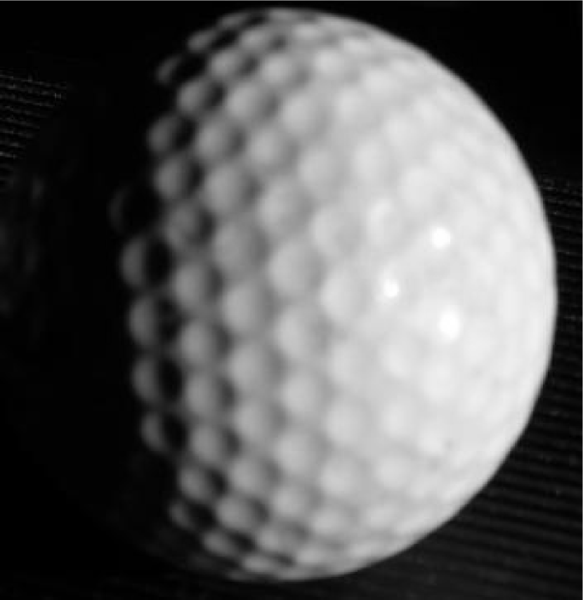
Figure 1.— Physical analog of the cratered asteroid model, seen at $\sim 60^{\circ}$ phase angle. In the actual computational model the flat areas between the craters are eliminated.

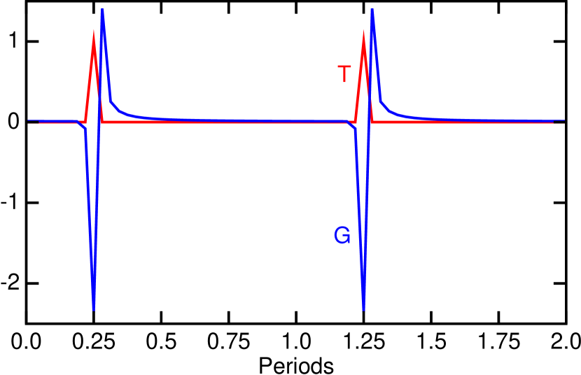
Figure 2.— Heat flow into the surface ($G$) for a triangle temperature forcing function $T$. Computed with 32 samples per period. Two full cycles are shown.

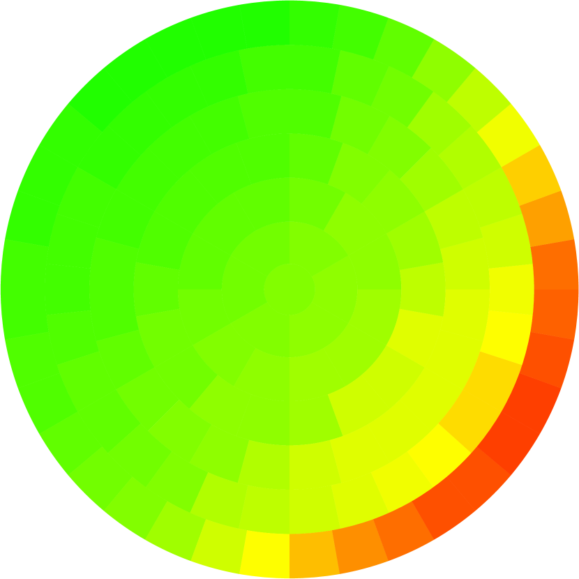
Figure 3.— Temperature distribution in the late afternoon for a crater at $4^{/}circ$ latitude when the sub-solar latitude is $30^{\circ}$. The thermal inertia parameter is $\Theta=1$. The Sun is setting in the Northwest, so the Southeast rim of the crater is still sunlit.

Figure 4.— Infrared phase curves for an asteroid 1.4 AU from the Sun in the passbands of the IRAC on the Spitzer Space Telescope, 3.6, 4.5, 5.6 & 8 $\mu$m from bottom to top. The solid curves show a cratered model with maximum slope $\theta_{max}=45^{\circ}$, while the dotted curves show an uncratered model. The dashed line shows the 0.01 mag/degree phase curve of the STM.

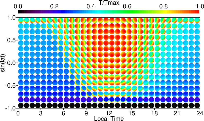
Figure 5.— Temperature distribution as a function of latitude and local time for a rotating cratered model with thermal inertia parameter $\Theta=0.1$ and maximum crater slope $\theta_{max}=45^{\circ}$. The sub-solar latitude is $30^{\circ}$.

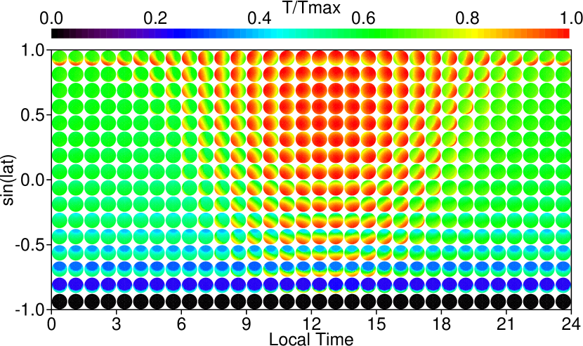
Figure 6.— Temperature distribution as a function of latitude and local time for a rotating cratered model with thermal inertia parameter $\Theta=1$ and maximum crater slope $\theta_{max}=45^{\circ}$. The sub-solar latitude is $30^{\circ}$. The circle just above the equator at local time 17:37 is blown up in Figure 3.

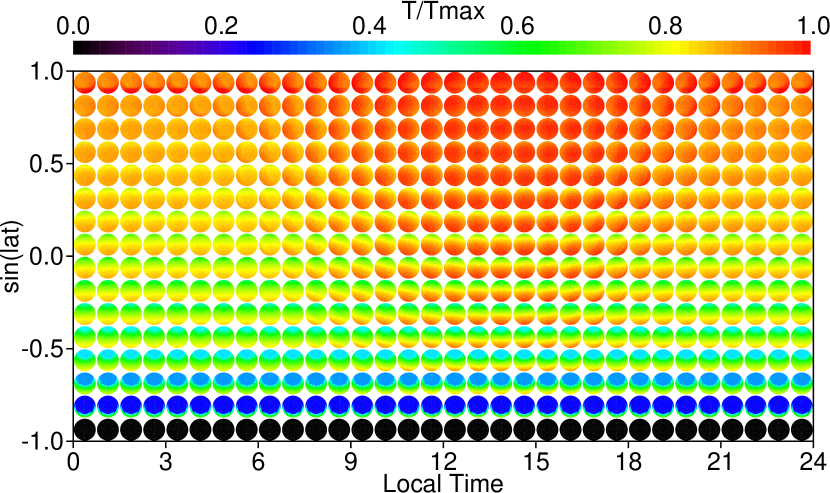
Figure 7.— Temperature distribution as a function of latitude and local time for a rotating cratered model with thermal inertia parameter $\Theta=10$ and maximum crater slope $\theta_{max}=45^{\circ}$. The sub-solar latitude is $30^{\circ}$.

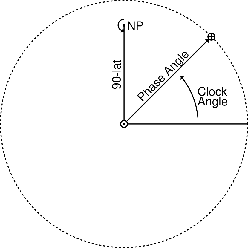
Figure 8.— Definition of the clock angle. $\odot$ marks the sub-solar point, and $\oplus$ marks the sub-observer point. The angle between the pole and the sub-solar point is $90-\beta_{\odot}$.

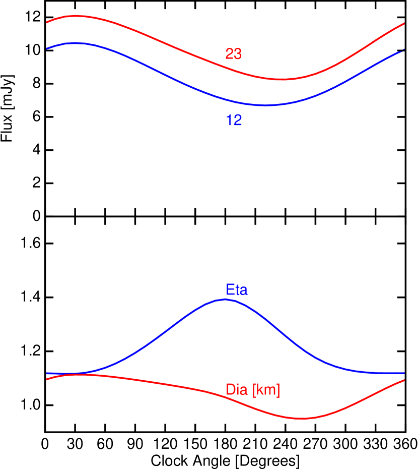
Figure 9.— Flux in the WISE 12 and 23 $\mu$m bands for a 1 km asteroid 1 AU from the Earth and 1.4 AU from the Sun, observed at $50^{\circ}$ phase angle. The sub-solar latitude is $30^{\circ}$ and the thermal inertia parameter is $\Theta=1$. The clock angle rotates the line of sight around the Sun line while keeping a constant phase angle. For $0^{\circ}$ clock angle the observer is East of the Sun, giving an afternoon view. For $90^{\circ}$ clock angle the observer is over $80^{\circ}$ latitude at noon. These fluxes lead to a beaming parameter $\eta$ and calculated diameter $D$ using the NEATM.

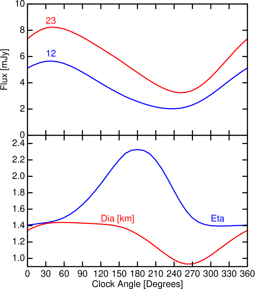
Figure 10.— As in Figure 9, but at $90^{\circ}$ phase angle. For $0^{\circ}$ clock angle the observer is over the equator at 6 PM. For $90^{\circ}$ clock angle the observer is over $60^{\circ}$ latitude at midnight.

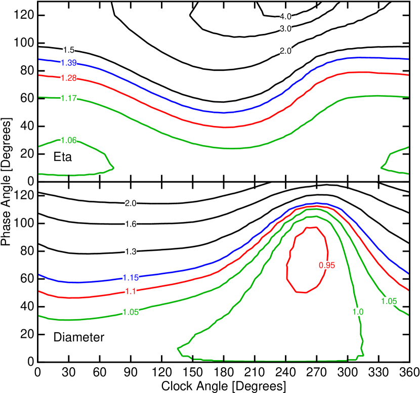
Figure 11.— The beaming parameter $\eta$ and the fitted diameter as a function of the phase and clock angles for the asteroid in Figure 9.

Figure 12.— Histogram showing the frequency of various diameter discrepancies when using the NEATM to analyze fluxes from the rotating cratered model, assuming spherical asteroids.

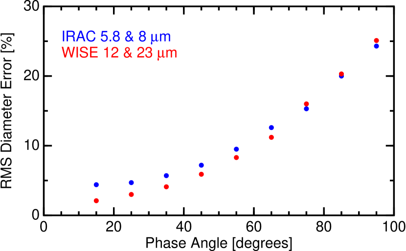
Figure 13.— RMS diameter errors for a sample of 576 NEOs that could be observed by the Spitzer Space Telescope in Cycle 4. While the distance from the the Sun and phase angle are held fixed at the actual values, fluxes were simulated for Monte Carlo asteroids with random thermal inertias uniform in pole position and $\log\Theta$ in the range $0.1<\Theta<10$. Fluxes at the WISE 12 & 23 $\mu$m bands gave NEATM RMS diameter errors shown by the lower dots. The IRAC 5.8 and 8 $\mu$m fluxes give the upper dots.

Figure 14.— The egg shaped example. The figure is rotationally symmetric about the horizontal axis, while the object rotates about a vertical axis.

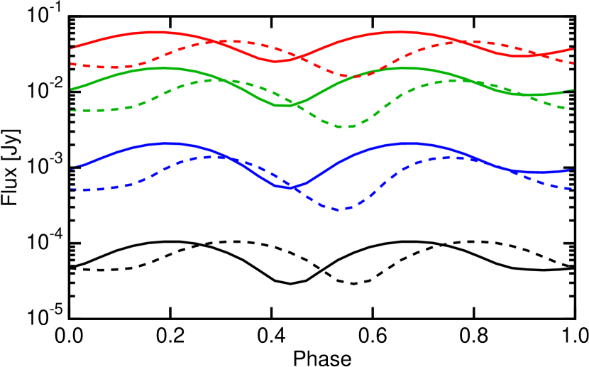
Figure 15.— Lightcurves for the egg shaped asteroid seen at $45^{\circ}$ phase angle with the rotation axis normal to the Earth-Sun-asteroid plane. The solid curves show viewing the afternoon side, while the dashed curves show the morning side. Black is optical, blue is 3.6 $\mu$m, green is 5.8 $\mu$m, and red is 12 $\mu$m.

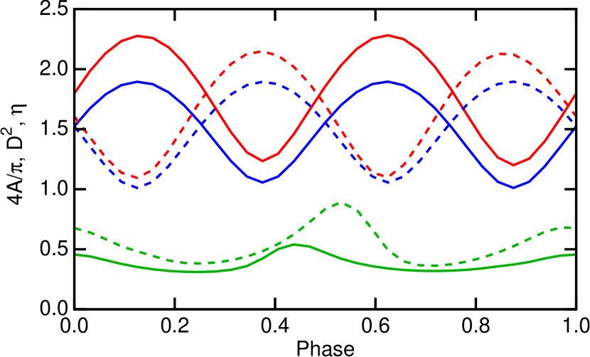
Figure 16.— The variations of the projected area in blue, the square of the NEATM derived diameter in red, and the NEATM $\eta$ parameter in green.

Figure 17.— Histogram showing the frequency of various diameter discrepancies when using the NEATM to analyze fluxes from the rotating cratered egg-shaped model. The solid histogram shows the distribution of diameter errors derived from single observations at a random rotational phase. The dashed histogram shows the distribution of diameter errors derived from the average over a rotation. The dotted curve shows a Gaussian with a 10% standard deviation.

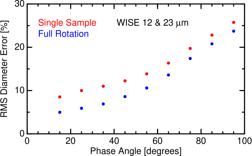
Figure 18.— RMS diameter errors for a sample of 576 NEOs that could be observed by the Spitzer Space Telescope in Cycle 4. While the distance from the the Sun and phase angle are held fixed at the actual values, fluxes were simulated for Monte Carlo asteroids with random thermal inertias uniform in pole position and $\log\Theta$ in the range $0.1<\Theta 10$. Fluxes at the WISE 12 & 23 $\mu$m bands were used in the NEATM. RMS diameter errors when a single observation is made of each asteroid give the upper dots, while errors after averaging the NEATM diameter give the lower dots.

In the rotating cratered asteroid model, heat is conducted vertically into and out of the surface, but not horizontally. The facets in a given crater can see each other and see the Sun, but there is no radiative transfer of heat from one crater to another. Thus the problem of finding the temperature distribution on the asteroid breaks up into many small problems of finding the temperature vs. time of each facet.

The equation describing heat conduction in the surface layer is

$$C\rho{{\partial T}\over{\partial t}}=\kappa{{\partial^{2}T}\over{\partial z^{2}}}$$ (1)

where $\kappa$ is the thermal conductivity, $\rho$ is the density, and $C$ is the specific heat per unit mass. The heat flow into the surface is $\kappa{{\partial T}\over{\partial z}}$. Letting $\zeta=z/\kappa$, then the heat flow is ${{\partial T}\over{\partial\zeta}}$ and the heat conduction equation is

$$\kappa\rho C{{\partial T}\over{\partial t}}={{\partial^{2}T}\over{\partial\zeta^{2}}}$$ (2)

which depends only on the thermal inertia $\Gamma=\sqrt{\kappa\rho C}$. The units of $\Gamma$ are $[E/(t(T/L)L^{2})M/L^{3}E/(TM)]^{1/2}=E/(TL^{2}\sqrt{t})$. In Wright (1976) the value of $\Gamma=0.006\;\mbox{cal/cm${}^{2}$/K/sec${}^{1/2}$}$ was used for Mars. In more modern units this is $251\;\mbox{J/m${}^{2}$/K/sec${}^{1/2}$}$. Harris (2006) gives values for $\Gamma$ of 10-20 for main belt asteroids, 50 for the Moon, 150 & 350 for the NEOs Eros & Itokawa, and $2500\;\mbox{J/m${}^{2}$/K/sec${}^{1/2}$}$ for bare rock.

Putting in the solar heating and thermal radiation, I get

$${{(1-A)L_{\odot}}\over{4\pi R^{2}}}\max(0,\cos\theta)-\epsilon\sigma T^{4}={{\partial T}\over{\partial\zeta}}$$ (3)

with $\theta=\Omega t$ where $\Omega$ is the rotational frequency of the asteroid, $R$ is the distance of the asteroid from the Sun, $L_{\odot}$ is the solar luminosity, $A$ is the albedo, $\epsilon$ is the emissivity in the thermal infrared, and $\sigma$ is the Stephan-Boltzmann constant. This assumes the special case of an equatorial region with the sub-solar latitude ($\beta_{\odot}$) of zero. In general the $\max(0,\cos\theta)$ would be replaced by either the cosine of the angle between the Sun and the surface normal, or zero if the facet is shadowed on the Sun is below the horizon.

The unit of temperature in the code is

$$T_{\circ}=\left({{(1-A)L_{\odot}}\over{4\pi\epsilon\sigma R^{2}}}\right)^{1/4}$$ (4)

which is the equilibrium temperature of a surface oriented toward the Sun. Let $y=T/T_{\circ}$, giving

$$\epsilon\sigma T_{\circ}^{3}[\max(0,\cos\theta)-y^{4}]={{\partial y}\over{\partial\zeta}}$$ (5)

and

$$\kappa\rho C\Omega{{\partial y}\over{\partial\theta}}={{\partial^{2}y}\over{\partial\zeta^{2}}}$$ (6)

Redefine the depth variable again using $w=\epsilon\sigma T_{\circ}^{3}\zeta=z/H$ where $H$ is the distance such that a temperature gradient of $T_{\circ}/H$ sets up a conductive flux equal to the radiative flux $\epsilon\sigma T_{\circ}^{4}$. These equations are now

$$\max(0,\cos\theta)-y^{4}={{\partial y}\over{\partial w}}$$ (7)

and

$${{\kappa\rho C\Omega}\over{(\epsilon\sigma T_{\circ}^{3})^{2}}}{{\partial y}\over{\partial\theta}}={{\partial^{2}y}\over{\partial w^{2}}}.$$ (8)

The coefficient

$$\Theta={{\sqrt{\kappa\rho C\Omega}}\over{\epsilon\sigma T_{\circ}^{3}}}={{\Gamma\sqrt{\Omega R^{3}}}\over{(\epsilon\sigma)^{1/4}[(1-A)L_{\odot}/4\pi]^{3/4}}}$$ (9)

is a dimensionless measure of the importance of thermal inertia on the temperatures. It is about $\Theta=1.5$ for Mars using the parameters of Wright (1976).

Now let $y=\sum_{n}y_{n}\exp(in\theta-k_{n}w)$. The solutions to the equation

$$\Theta^{2}{{\partial y}\over{\partial\theta}}={{\partial^{2}y}\over{\partial w^{2}}}$$ (10)

must have $in\Theta^{2}=k_{n}^{2}$ so $k_{n}=\Theta\sqrt{n/2}(1+i)$ for $n>0$. For negative $n$, $k_{n}=\Theta\sqrt{|n|/2}(1-i)$ must be taken to guarantee the solution is damped toward $z=\infty$.

The physical length scale given by $H/\Theta=\Gamma/(C\rho\sqrt{\Omega})$. Since $C\rho\approx 10^{6}\;\mbox{J/m${}^{3}$/K}$ and $\Omega\approx 10^{-4}\;\mbox{rad/sec}$, the length scale is smaller than 10 cm. Thus the assumption of no horizontal heat conduction is reasonable for craters $>1\;\mbox{m}$.

The heat flow into the surface is

$${{\partial y}\over{\partial w}}=-\sum_{n}y_{n}k_{n}\exp(in\theta).$$ (11)

Now take $y(\theta,0)$ as a triangle wave centered at $\theta=0$ with $y=1$, and linearly sloping down to $y=0$ at $\theta=\pm 2\pi/N$. This gives

$$y_{n} = \pi^{-1}\int_{0}^{2\pi/N}\cos(n\theta)(1-N\theta/2\pi)d\theta$$ (12)

$$= {{N(1-\cos(2\pi n/N))}\over{2\pi^{2}n^{2}}}$$

The heat flow into the surface is $\Theta G(\theta)$ with

$$G(\theta)=\sum_{n=1}^{\infty}{{N(1-\cos(2\pi n/N))}\over{2\pi^{2}n^{2}}}\sqrt{2n}(\sin n\theta-\cos n\theta)$$ (13)

The value of this $G(\theta)$ at $\theta=2\pi m/N$ defines the vector $G$ used in code. The average of this over bins of width $2\pi/N$ in $\theta$ centered $\theta=2\pi m/N$ is:

$$\overline{G(m)} = \sum_{n=1}^{\infty}{{N^{2}(1-\cos[2\pi n/N])\sin[\pi n/N]}\over{\sqrt{2}\pi^{3}n^{2.5}}}$$ (14)

$$\times \left(\sin\left[{{2\pi nm}\over{N}}\right]-\cos\left[{{2\pi nm}\over{N}}\right]\right)$$

Figure 2 shows the function $\overline{G(m)}$ for $N=32$.

The mutual irradiation of the crater facets introduces a coupling matrix. The contribution of facet $j$ to facet $i$ goes like $\pi^{-1}\Delta\Omega_{j}R^{2}\cos(\theta_{j})\cos(\theta)/d^{2}_{ij}$ where $\theta_{i}=\theta_{j}$ are the angle of emission and incidence, $\Delta\Omega_{j}$ is the solid angle of the facet on the spherical cap crater, and $d_{ij}=2R\cos(\theta_{j})$ is the distance between the facets. Thus the coupling is just $\Delta\Omega/4\pi$. The total light falling on a facet is given by

$$S_{i}=D_{i}+A\sum_{j}{{\Delta\Omega_{j}}\over{4\pi}}S_{j}=D_{i}+{{A\Omega_{crater}}\over{4\pi}}\langle S\rangle.$$ (15)

where $D_{i}$ is the direct solar flux, and $S_{i}$ is the total flux on a facet. Averaging this equation gives

$$\langle S\rangle=\langle D\rangle+{{A\Omega_{crater}}\over{4\pi}}\langle S\rangle$$ (16)

so

$$\langle S\rangle={{\langle D\rangle}\over{1-A)f_{c}}}$$ (17)

where $f_{c}$ is $\Omega_{crater}/4\pi$, the fraction of the sphere included in the spherical cap craters. For the $\theta_{max}=45^{\circ}$ used here, $f_{c}=(1-\cos\theta_{max})/2=0.15$. Therefore

$$S_{i}=D_{i}+{{\langle D\rangle Af_{c}}\over{1-Af_{c}}}$$ (18)

For the calculations reported here, the craters were divided into 127 facets, consisting of a central circle surrounded by rings of 6, 12, …, 36 square facets. Since the resulting facet size of $2\theta_{max}/13\approx 7^{\circ}$ was fairly coarse, the direct insolation $D_{i}$ was computed as $\mu_{i}f_{v}$ times $F_{\odot}$, where $f_{v}$ is the fraction of the facet that is visible from the Sun, and $\mu$ is the cosine of the angle between the surface normal and the Sun. The visible fraction is computed using a finer pixelization of the sphere, HEALpix (Górski et al., 2005) with 49,152 pixels. Figure 3 shows the facet structure with a crater.

In the thermal infrared, the mutual visibility of the facets couples their temperatures together. The total infrared flux falling on a facet is

$$H_{i}=\sum_{j}{{\epsilon\sigma T_{j}^{4}\Delta\Omega_{j}}\over{4\pi}}+(1-\epsilon)f_{c}\langle H\rangle$$ (19)

Averaging this equation gives

$$H_{i}=<H>={{\epsilon\sigma\langle T^{4}\rangle f_{c}}\over{1-(1-\epsilon)f_{c}}}$$ (20)

Remembering that the unit of flux is both $(1-A)F_{\odot}$ and $\epsilon\sigma T_{\circ}^{4}$, and that only a fraction $\epsilon$ of the incident heat $H$ is absorbed, we get a power balance equation

$$y_{ij}^{4} = (f_{v}\mu)_{ij}+\frac{Af_{c}}{1-Af_{c}}n^{-1}\sum_{j}(f_{v}\mu)_{ij}$$ (21)

$$+ \frac{\epsilon f_{c}}{1-(1-\epsilon)f_{c}}n^{-1}\sum_{j}y_{ij}^{4}$$

$$+ \Theta\sum_{k}y_{ik}G_{[(k-j)\mbox{mod}N]}$$

where $y_{ij}$ is the temperature of the $i^{th}$ facet at the $j^{th}$ time, and there are $n$ facets and $N$ times. This is a set of $n\times N=127\times 32=4064$ coupled non-linear equations in 4064 variables. Fortunately the facet to facet coupling is weak and can be handled by iteration, so the task of solving for the temperatures is not too onerous.

There is little point in using extremely fine subdivisions of the asteroid’s surface. The brightness temperatures of Mars were calculated by Wright (1976) using only 6 latitudes. In the calculations reported here, 16 latitudes were used, and the rotation period was divided in 32 time steps. This gives 65,024 temperatures to be found. These temperature pattern are plotted in Figures 5, 6 & 7 for $\Theta$ values of 0.1, 1 & 10 with sub-solar latitude of $30^{\circ}$.

2.1. Observed Flux Calculation

Given the temperature distribution, the observed flux is found by integrating over the surface of the asteroid. For a given frequency $\nu$, the quantity $x_{\circ}=h\nu/kT_{\circ}$ is found. Then the observed infrared flux is found using

$$F_{\nu} = \frac{2\epsilon h\nu^{3}}{c^{2}}\sum_{\beta,j}\max(\mu_{f}(\beta,j),0)\frac{d\Sigma(\beta,j)}{D^{2}}$$ (22)

$$\times \frac{\sum_{i}(f_{v}\mu)_{ij\beta}(\exp(x_{\circ}/y_{ij\beta})-1)^{-1}}{\sum_{i}(f_{v}\mu)_{ij\beta}}$$

where $d\Sigma(\beta,j)$ is the surface area of the asteroid in the bin at latitude $\beta$ and longitude given by $j$, D is the distance to the observer, $\mu_{f}$ is the cosine of angle between the normal to the surface and the line of sight, and $(f_{v}\mu)_{ij\beta}$ is the fraction of the $i^{th}$ facet visible by the observer times the cosine of the angle between the facet normal and the line of sight. The observed bolometric optical flux is

$$F_{opt} = \sum_{\beta,j}\max(\mu_{f}(\beta,j),0)\frac{d\Sigma(\beta,j)}{D^{2}}$$ (23)

$$\times \frac{\sum_{i}(f_{v}\mu)_{ij\beta}AS_{ij\beta}/\pi}{\sum_{i}(f_{v}\mu)_{ij\beta}}$$

This can be multiplied by $F_{\nu}(\odot)/F_{bol}(\odot)$ to give the reflected optical spectrum.

In this paper the latitudes are uniformly spaced in $\sin\beta$, so $d\Sigma$ is a constant for a sphere. The assumption that the asteroid is spherical only enters into $d\Sigma$, so any convex shape for an asteroid can be accommodated merely by changing the weights $d\Sigma$ going into the flux sum. It is important to remember that the angles $\beta$ and $\lambda$ refer to the surface normal vector, not the vector from the center to a surface element. Thus at the end of the major axis of a $2:1:1$ ellipsoid, $d\Sigma$ is a minimum, 16 times smaller than the value at the end of the minor or intermediate axes.

3. NEATM Fitting

The rotating cratered asteroid model described model has been used to predict infrared fluxes for NEOs, and then these fluxes have been used in the NEATM to find the beaming parameter $\eta$ and the diameter $d$. For a given observation, the distance to the Sun and the phase angle are known, but there are still two angles and the thermal inertia parameter $\Theta$ that need to be specified. Figure 8 shows the definition of the two angles, which are the sub-solar latitude and the clock angle. Examples are shown in Figures 9 and 10 for a 1 km diameter asteroid 1.4 AU from the Sun, with albedo $A=0.1$ and emissivity $\epsilon=0.9$. At a $50^{\circ}$ phase angle, the errors in the NEATM calculated diameters are small, but for $90^{\circ}$ the maximum error increases by a factor of 4. These calculations have been done using the planned 12 & 23 $\mu$m bands of the Widefield Infrared Survey Explorer (WISE, (Mainzer et al., 2006)) which is scheduled for launch in 2009.

4. NEATM Accuracy

The NEATM can reproduce the model diameters for quite well for phase angles $\alpha<60^{\circ}$. Figure 11 shows that the errors are small for any clock angle as long as the phase angle is smaller than $60^{\circ}$. This conclusion does not depend strongly on either the sub-solar latitude or the thermal inertia parameter $\Theta$. To show this for a representative sample of real observations, Monte Carlo simulations of NEO observations from a Spitzer Space Telescope proposal (SNEAS, PI Eisenhardt). 576 NEOs were found to be observable by Spitzer during Cycle 4, with good signal-to-noise ratio in the IRAC 5.8 & 8 $\mu$m bands. Only the distance to the Sun and the phase angle were taken from this observation table. Then fluxes were computed for a random distribution of pole positions and thermal inertias. The pole positions were chosen uniformly in $4\pi$ steradians, and the thermal inertias were chosen uniformly in the logarithm in the range $0.1<\Theta<10$. To choose a random pole position one picks $\sin\beta_{\odot}$ uniform in $[0-1]$ and the clock angle uniform in $[0-2\pi]$. For each of the 576 objects 30 different choices of pole position and $\Theta$ were analyzed. The fluxes were then analyzed using the NEATM to derive $\eta$ and a diameter. The RMS diameter errors, binned by phase angles, are shown in Figure 13. Both the WISE 12 & 23 $\mu$m bands, and the Spitzer IRAC 5.8 & 8 $\mu$m bands give data that work well with the NEATM.

When the NEATM breaks down at large phase angles, the estimated diameter is usually too large. Figure 12 shows the distribution of the errors for the Monte Carlo observations in Figure 13. The distribution is clearly positively skewed.

Figure 13 shows that the NEATM works reasonably well for moderate phase angles when compared to a more complete thermophysical model. But to show that the NEATM works in the real world one needs comparisons to real objects with size determined by radar or spacecraft imaging. Harris & Lagerros (2002) find that NEATM diameter errors average less than 10% for phase angles less than $60^{\circ}$, but the number of objects in the comparison was quite small.

5. Asphericity

All of the previous caculations have assumed spherical objects, but small NEOs usually have quite aspherical shapes. An example of a non-spherical shape is the egg-shaped object seen in Figure 14. This is half of a 2.5:1:1 ellipsoid joined to half of a 1.25:1:1 ellipsoid. If this object is 1 AU from the Earth, and 1.414 AU from the Sun, with phase angle of $45^{\circ}$ and a sub-solar latitude of $0^{\circ}$, thermal inertia parameter $\Theta=1$, albedo of 0.1 and emissivity of 0.9, one gets the lightcurves seen in Figure 15 for clock angles of $0^{\circ}$ and $180^{\circ}$. The flux normalization applies to a 1 km short axis and a 1.875 km long axis. The optical lightcurve amplitude is 1.4 mag peak to peak while the 23 $\mu$m amplitude is 0.84 to 0.93 mag. These amplitudes are larger than the 1.875:1 variation in the projected area for this shape. The NEATM applied to the 12 and 23 $\mu$m data gives the $\eta$ and $D$ values plotted in Figure 16 along with the projected area as a function of rotational phase. The diameter from the NEATM tracks the projected area fairly well, and there is a definite variation of the beaming parameter $\eta$ with rotational phase.

The calculations of the accuracy of the NEATM for the Spitzer sample of 576 NEOs have been repeated for the egg-shaped asteroid shown in Figure 14. A non-spherical shape introduces another parameter, the rotational phase, that must be either treated as a random variable or integrated over. Figure 17 compares NEATM diameters to the true “diameter” of the egg. There are many ways to define the true diameter: the diameter of the sphere with the same volume of the egg is 1.233 km, while the sphere with the same surface area as the egg has a diameter of 1.275 km. Since the NEATM is trying to estimate the projected area of an object it seems reasonable to use the equivalent area diameter of 1.275 km as the reference.

Even a single sample at a random rotational phase gives a reasonable diameter estimate: the ratio of the NEATM to equivalent area sphere has a median and interquartile range of $1.042^{+0.075}_{-0.096}$. Since the interquartile range only contains 50% of the sample, these errors should be considered to be standard errors instead of standard deviations. One can do better using the NEATM diameter averaged over the rotation period. This gives a median ratio and interquartile range of $1.019^{+0.082}_{-0.072}$. The improvement coming from better sampling of the rotational phase is fairly small, even though the egg shape considered here gives high peak to peak amplitudes up to 1.4 mag in the optical and short infrared wavelengths. The small amplitude in diameters is due to several factors: the lightcurve amplitude is lower at the WISE wavelengths of 12 and 23 $\mu$m, the rms of a sine wave is 2.8 times less than the peak to peak, the amplitude goes down to zero for pole-on orientations, and the diameter varies like the square root of the flux. The median and interquartile range of the rms variation of the NEATM diameter with rotational phase is only $7.6^{+3.0}_{-3.9}$ percent, while the median peak to peak 12 $\mu$m flux amplitude is 0.647 mag.

It is better to evaluate the diameter at each rotational phase using the NEATM and average these diameters than to average the fluxes and use these averages in the NEATM. The RMS errors for both single sample and rotationally averaged NEATM diameters for the sample of NEOs observable by Spitzer are shown in Figure 18. For each asteroid, 30 different pole positions and inertia parameters $\Theta$ have been simulated, using the egg-shaped model discussed above.

6. Conclusion

The errors in diameters computed from the NEATM for asteroid observations at phase angles less than $60^{\circ}$ are less than 10% RMS, even for the non-spherical shapes typical of NEOs. For WISE, observing at $90^{\circ}$ elongation, any object with a distance larger than 0.6 AU will have a phase $\alpha<60^{\circ}$. The Spitzer Space Telescope can observe at elongations between $85^{\circ}$ and $120^{\circ}$, so only very close passes involve $\alpha>60^{\circ}$. The error evaluated in this paper only includes the errors due to not knowing the thermal inertia and pole orientation of an asteroid. There will be additional errors due to uncertainties in the true emissivity of the asteroid surface, but these errors should be small, since the emissivities in the thermal infrared are quite close to the maximum possible value of 1.0. Diameters from the NEATM do not depend on the assumed albedo so there is no additional error from albedos. WISE will obtain $\approx 10$ observations of each asteroid spread over 30 hours, and will thus get good sampling of asteroid lightcurves, which reduces the errors associated with non-spherical shapes. WISE will be sensitive enough to measure hundreds of thousands of asteroids, and fitting the WISE 12 & 23 $\mu$m fluxes using the NEATM will provide reasonably good diameter limits for a large sample of asteroids.

7. Acknowledgements

Josh Emery and Alan Harris (DLR) provided useful comments and suggestions. Research on WISE at UCLA is supported by the Astrophysics Division of the NASA Science Mission Directorate.

References

- Górski et al. (2005) Górski, K. M., Hivon, E., Banday, A. J., Wandelt, B. D., Hansen, F. K., Reinecke, M., Bartelmann, M. 2005. HEALPix: A Framework for High-Resolution Discretization and Fast Analysis of Data Distributed on the Sphere. Astrophysical Journal 622, 759-771.
- Hansen (1977) Hansen, O. L. 1977. An Explication of the Radiometric Method for Size and Albedo Determination. Icarus 31, 456-482.
- Harris (1998) Harris, A. W. 1998. A Thermal Model for Near-Earth Asteroids. Icarus 131, 291-301.
- Harris & Lagerros (2002) Harris, A.W. & Lagerros, J.S.V. 2002. Asteroids in the thermal IR. In: Bottke, W. F., Cellino, A., Paolicchi, P., Binzel, R. P. (Eds.), Asteroids III. Univ. of Arizona Press, Tucson, AZ, pp. 205-218.
- Harris (2006) Harris, A. W. 2006. The surface properties of small asteroids from thermal-infrared observations. In: Lazzaro, D., Ferraz-Mello, S., Fernandez, J. A. (Eds.), Proc. of IAU Symposium 229. Cambridge University Press, Cambridge, UK, pp. 449-463.
- Lagerros (1996) Lagerros, J. S. V. 1996. Thermal physics of asteroids. I. Effects of shape, heat conduction and beaming.. Astronomy and Astrophysics 310, 1011-1020.
- Lebofsky et al. (1986) Lebofsky, L. A., Sykes, M. V., Tedesco, E. F., Veeder, G. J., Matson, D. L., Brown, R. H., Gradie, J. C., Feierberg, M. A., Rudy, R. J. 1986. A refined ‘standard’ thermal model for asteroids based on observations of 1 Ceres and 2 Pallas. Icarus 68, 239-251.
- Mainzer et al. (2006) Mainzer, A. K., Eisenhardt, P., Wright, E. L., Liu, F.-C., Irace, W., Heinrichsen, I., Cutri, R., Duval, V. 2006. Update on the Wide-Field Infrared Survey Explorer (WISE). Space Telescopes and Instrumentation I: Optical, Infrared, and Millimeter. Edited by Mather, John C.; MacEwen, Howard A.; de Graauw, Mattheus W. M.. Proceedings of the SPIE, Volume 6265, pp. 626521 (2006).
- Morbidelli et al. (2002a) Morbidelli, A., Jedicke, R., Bottke, W. F., Michel, P., and Tedesco, E. F. 2002a. From Magnitudes to Diameters: The Albedo Distribution of Near Earth Objects and the Earth Collision Hazard. Icarus 158, 329-342.
- Peterson (1976) Peterson, C. 1976. A source mechanism for meteorites controlled by the Yarkovsky effect. Icarus 29, 91-111.
- Veeder et al. (1989) Veeder, G. J., Hanner, M. S., Matson, D. L., Tedesco, E. F., Lebofsky, L. A., Tokunaga, A. T. 1989. Radiometry of near-earth asteroids. Astronomical Journal 97, 1211-1219.
- Vokrouhlicky (1999) Vokrouhlicky, D. 1999. A Complete Linear Model for the Yarkovsky Thermal Force on Spherical Asteroid Fragments. Astronomy & Astrophysics 344, 362-366.
- Wright (1976) Wright, E. L. 1976. Recalibration of the far-infrared brightness temperatures of the planets. Astrophysical Journal 210, 250-253.