Abstract

Non-Common Path Aberrations (NCPA) are one of the main limitations for extreme Adaptive Optics (AO) system. NCPA prevent extreme AO systems to achieve their ultimate performance. These static aberrations are unseen by the wave front sensor and therefore not corrected in closed loop. We present experimental results validating new procedures of measurement and pre-compensation of the NCPA on the AO bench at ONERA. The measurement procedure is based on new refined algorithms of phase diversity. The pre-compensation procedure makes use of a pseudo-closed loop scheme to overcome the AO wavefront sensor model uncertainties. Strehl Ratio obtained in the images reaches 98.7 % @ 632.8 nm. This result allows us to be confident of achieving the challenging performance required for extrasolar planet direct observation.

OCIS codes: 010.1080, 010.7350, 100.5070, 100.3190

1 Introduction

Exoplanet direct imaging is one of the leading goal of today’s astronomy. Such a challenge with a ground-based telescope can only be tackled by a very high performance Adaptive Optics (AO) system, so-called eXtreme AO (XAO), a coronagraph device, and a smart imaging process .${}^{\hbox{\immediate{\bf{?}},\penalty 1000\hskip 0.91003pt plus 0.70004pt minus 0.70004pt{\bf{?}}}}$ Most of the large telescopes are nowadays equipped with AO systems able to enhance their imaging performance up to the diffraction limit. One of the limitations of the existing AO system performance remains the unseen Non-Common Path Aberrations (NCPA). These static optical aberrations are located after the beam splitting, in the Wave-Front Sensor (WFS) path and in the imaging path.

The correction of NCPA is one of the critical issues to achieve ultimate system performance ${}^{\hbox{\immediate{\bf{?}}}}$ for XAO. These aberrations have to be measured by a dedicated WFS tool, judiciously placed in the imaging camera focal plane, and then directly pre-compensated in the closed loop process. An efficient way to obtain such a calibration is to use a Phase Diversity (PD) algorithm ${}^{\hbox{\immediate{\bf{?}},\penalty 1000\hskip 0.91003pt plus 0.70004pt minus 0.70004pt{\bf{?}},\penalty 1000\hskip 0.91003pt plus 0.70004pt minus 0.70004pt{\bf{?}}}}$ for the NCPA measurement.

For the correction, the Wave-Front (WF) references of the AO loop can be modified to account for these unseen aberrations in the AO compensation and to directly obtain the best possible wave-front quality at the scientific detector .${}^{\hbox{\immediate{\bf{?}}}}$

This type of approach has been successfully applied on NAOS-CONICA ${}^{\hbox{\immediate{\bf{?}}}}$ or Keck ${}^{\hbox{\immediate{\bf{?}}}}$ and has led to a significant gain of global system performance .${}^{\hbox{\immediate{\bf{?}}}}$ Even if a real improvement can be seen on pre-compensated images, a significant amount of aberrations are still not corrected. In the frame of the SPHERE instrument development ,${}^{\hbox{\immediate{?}}}$ we propose an optimized procedure in order to significantly improve the efficiency of the NCPA calibration and pre-compensation for high contrast imaging. The goal is to achieve a residual Wave-Front Error (WFE) NCPA contribution of less than 10 nm RMS after pre-compensation.

The principle of the conventional procedure, as used in NAOS-CONICA ,${}^{\hbox{\immediate{\bf{?}},\penalty 1000\hskip 0.91003pt plus 0.70004pt minus 0.70004pt{?}}}$ is recalled and commented in Section 2. The newly optimized algorithm for the NCPA measurements is described in Section 3 and is based on a Maximum A Posteriori approach (MAP) ${}^{\hbox{\immediate{\bf{?}},\penalty 1000\hskip 0.91003pt plus 0.70004pt minus 0.70004pt{\bf{?}}}}$ for the phase estimation. The new approach for the NCPA pre-compensation is presented in Section 4. The application of the PD by the DM itself is discussed in Section 5. In Section 6, we detail the experimental results obtained with the ONERA AO bench for the validation of the key points of the proposed NCPA calibration and pre-compensation procedure.

2 Principle of the NCPA calibration and pre-compensation

2.A Phase diversity for NCPA calibration

In order to directly measure the wave front errors at the level of the scientific detector, a dedicated WFS has to be implemented. The idea is to avoid any additional optics. The WFS must therefore be based on the processing of the focal plane images recorded by the scientific camera itself. The phase diversity (PD) approach ${}^{\hbox{\immediate{?},\penalty 1000\hskip 0.91003pt plus 0.70004pt minus 0.70004pt{?},\penalty 1000\hskip 0.91003pt plus 0.70004pt minus 0.70004pt{?},\penalty 1000\hskip 0.91003pt plus 0.70004pt minus 0.70004pt{?}}}$ is a simple and efficient candidate to perform such a measurement. In this section we are going to briefly describe the PD concept and its interest with respect to our particular problematic.

The principle of PD (as shown in Figure 1) is to use two focal plane images differing by a known aberration (for instance defocus), in order to estimate the aberrated phase.

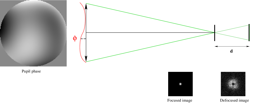
Fig. 1: Principle of phase diversity : two images differing by a known aberration (here defocus).

As shown in Equation 2.1, the two images recorded on the imaging camera are nothing but the convolution of the object and the PSF (the PSF being related to the pupil phase $\phi$) plus photon and detector additive noises:

$$i_{f} = \left|FT^{-1}\left(P\exp(j\phi)\right)\right|^{2}*o+n$$

$$i_{d} = \left|FT^{-1}\left(P\exp(j(\phi+\phi_{d}))\right)\right|^{2}*o+n$$ (2.1)

where $i_{f}$ is the conventional image, $i_{d}$ the PD image, $j=\sqrt{-1}$, $P$ the pupil function, $\phi$ the unknown phase, $\phi_{d}$ the known aberration, $o$ the observed object, $n$ the total noise, $*$ stands for the convolution process, and $FT$ stands for Fourier Transform. The phase $\phi(\vec{\rho})$ is generally expanded on a set of basis modes ($\vec{\rho}$ the position vector in the pupil plane). Using the Zernike basis to describe the aberrated phase we can write:

$$\phi(\vec{\rho})=\Sigma_{k}a_{k}\cdot Z_{k}(\vec{\rho})$$ (2.2)

where $a_{k}$ are the Zernike coefficients of the phase expansion and $Z_{k}$ the Zernike polynomials. The number of $a_{k}$ used to describe the phase will depend on the performance required and on the SNR characteristics. Nevertheless, since optical aberrations are considered, only first Zernike (typically between 10 to 100) are enough to well describe the NCPA.

As shown in Equation 2.1, there is a nonlinear relation between $i_{f}$ and $\phi$ (and thus the $a_{k}$ coefficients). The estimation of $\phi$ has to be solved by the minimization of a given criterion .${}^{\hbox{\immediate{?},\penalty 1000\hskip 0.91003pt plus 0.70004pt minus 0.70004pt{?}}}$ We propose hereafter to define an optimal criterion adapted to the instrumental conditions (noise and WF aberrations) by using a MAP approach.

The most simple known aberration to apply is a defocus ,${}^{\hbox{\immediate{?}}}$ (its amplitude is typically of the order of $\lambda$) which can be introduced in several ways :

• by translating the camera detector itself along the optical axis. The drawback of this approach is the range of displacement required for the detector, especially when high F ratio are considered. But this theoretically is the best option if it can be implemented. All the other options, presented below, may introduce not only defocus, but other high order aberrations of very low amplitudes, especially spherical aberration ($Z_{11}$). Even if they are easily quantified by using optical design software, they may, in fine, limit the accuracy of the calibration.

• by translating a pinhole source in the entrance focal plane of the camera. This option has been used to calibrate the NCPA on CONICA .${}^{\hbox{\immediate{?},\penalty 1000\hskip 0.91003pt plus 0.70004pt minus 0.70004pt{?}}}$

• by defocusing the image of a pinhole source in the entrance focal plane of the camera by translating the upstream collimator, for instance.

• and last but not least by using the DM directly. An adequate application of a set of voltages on the DM allows us to introduce the wanted defocus with an accuracy related to the DM fitting capability.

The two main advantages of the DM option are:

• no additional optical device is installed in the instrument, e.g. a software procedure may be developed to properly offset the voltages of the DM,

• other types of aberrations, like astigmatism for instance, can also be considered leading to a high flexibility in the procedure. Moreover, introducing other aberrations allows more accurate estimation of the focus itself as presented in section 5.

The DM option was first used in NAOS-CONICA${}^{\hbox{\immediate{?},\penalty 1000\hskip 0.91003pt plus 0.70004pt minus 0.70004pt{?}}}$ and has also been applied to Keck.${}^{\hbox{\immediate{?}}}$ A number of limitations have been identified in the PD:${}^{\hbox{\immediate{?},\penalty 1000\hskip 0.91003pt plus 0.70004pt minus 0.70004pt{?}}}$ photon and detector noise, detector defects (flat field stability), accuracy of the PD (amplitude and possibly additional high order aberrations) and algorithm approximations ${}^{\hbox{\immediate{?}}}$ (including the number of Zernike). In the optimized procedure we propose hereafter, the phase estimation is performed by minimizing a Maximum A Posteriori criterion accounting for non-uniform noise model and phase a priori in a regularization term (see ${}^{\hbox{\immediate{?}}}$ for a detailed explanation of this approach). This optimized PD algorithm is presented in section 3.

2.B NCPA pre-compensation in the AO loop

The principle of the NCPA pre-compensation is presented in Figure 2. It consists in modifying the reference of the WFS to deliver a pre-compensated wave-front to the scientific path.

A two steps process is therefore considered. Reference slopes are computed from PD data using a WFS model.${}^{\hbox{\immediate{\bf{?}}}}$ For that, a NCPA slope vector, as would be measured by the AO WFS (a Shack Hartmann for instance), is first computed off-line from the PD-measured set of Zernike coefficients by a matrix multiplication.

The new reference vector is then added to the current WFS reference. Then closing the AO loop on the reference allows us to apply the opposite of the NCPA to the DM. This leads to the compensation for the scientific camera aberrations (in addition to the turbulence) and the enhancement of the image quality at the level of its detector.

Any error in the WFS model directly affects the reference modifications, computed from the measured NCPA, and thus limits the performance of the pre-compensation process. Model errors have been identified as an important limitation of the approach in NAOS-CONICA.${}^{\hbox{\immediate{?}}}$ As an example, an error of 10% on the pixel scale of the AO WFS detector directly translates into a 10% uncorrected amplitude of the NCPA. One way to reduce these model errors is to perform accurate calibrations of the WFS parameters. Nevertheless, uncertainties on calibrations (pixel scale of WFS, pupil alignment) will always degrade the ultimate performance of the pre-compensation process. In order to overcome this problem, a new robust approach is proposed in Section 3.

Fig. 2: Principe of NCPA pre-compensation.

An important parameter in the NCPA pre-compensation is the selected number of Zernike to be compensated by the DM. This number is in fact limited by the finite number of actuators of the DM, i.e. the finite number of degrees of freedom of the AO system. The DM can not compensate for all the spatial frequencies in the aberrant phase. In addition, the actuator geometry does not really fit properly the spatial behavior of the Zernike polynomials. All these problems are translated in fitting and aliasing errors on the compensated WF. These limitations have to be taken into account in the implementation of the pre-compensation procedure. It will be discussed later on in Section 6.

3 Optimization of the NCPA measurement

3.A Optimization of the PD algorithm

As shown in Equation 2.1, there is no linear relation between $i$ and $\phi$. Therefore, the estimation of $\phi$ requires the iterative minimization of a given criterion. We propose here to define an optimal criterion adapted to our experimental conditions (noise and phase to estimate) by using a MAP approach .${}^{\hbox{\immediate{?},\penalty 1000\hskip 0.91003pt plus 0.70004pt minus 0.70004pt{?}}}$

The MAP criterion is based on a bayesian scheme (see Equation 3.1) in which one wants to maximize the probability of having object $o$ and phase $\phi$ knowing the images $i_{f}$ and $i_{d}$.

$$P(o,\phi|i_{f},i_{d})=\frac{P(i_{f},i_{d}|o,\phi)P(o)P(\phi)}{P(i_{f})P(i_{d})}$$ (3.1)

The decomposition of this probability makes different terms appear as discussed in detail in the following paragraphs.

The denominator term $P(i_{f})P(i_{d})$ stands for the probability of obtaining the images $i_{f}$ and $i_{d}$. As the images are already measured, this term is equal to 1.

The term $P(i_{f},i_{d}|o,\phi)$, called “likelihood term”, represents the probability to obtain the measured data considering real object and phase. It is no more than the noise statistic in the image. The two main sources of noise are the detector noise and the photon noise:

• for high flux pixels in the image, the dominant noise is the photon one. Hence, it follows a Poisson statistical law which can be approximated by a non-uniform Gaussian law with a variance $\sigma_{i}^{2}(\vec{r})\simeq i(\vec{r})$, as soon as $i(\vec{r})$ is greater than a few photons per pixel. ($\vec{r}$ a position vector in the focal plane)

• for low flux pixels, the dominant noise is the detector noise, described by a spatially uniform distribution (same variance $\sigma_{e}^{2}$ for each pixel) and a gaussian statistical law.

Therefore, the global noise statistics can be approximated by a non-uniform gaussian law of variance ${}^{\hbox{\immediate{?}}}$ $\sigma_{i}^{2}(\vec{r})=\sigma_{e}^{2}+i(\vec{r})$.

The second term, $P(o)$, represents the a priori knowledge we have on the object. In our case, the object is marginally resolved (less than two pixels, for a diffraction FWHM of 4 pixels). Nevertheless to account for its small extension as well as to account for pixel response, we have chosen to consider it as an unknown in the PD process.

In the following, the only prior imposed on the object will be a positivity constraint (using a reparametrisation : $o=a^{2}$) leading to $P(o)=P(a^{2})=1$. The probability $P(o)$ does not impact on the criterion minimization.

The third term, $P(\phi)$, is the regularization term for the phase estimation. It accounts for the knowledge we have on the NCPA. Note that in our case we have chosen to parameterize the phase $\phi$ by the coefficients $a_{k}$ of its expansion on the Zernike basis. Then, the term $P(\phi)$ will easily solve the problem of the choice of the number of Zernike to be accounted for in the estimation of the phase. Let us mention that in the conventional PD approach ,${}^{\hbox{\immediate{?},\penalty 1000\hskip 0.91003pt plus 0.70004pt minus 0.70004pt{?},\penalty 1000\hskip 0.91003pt plus 0.70004pt minus 0.70004pt{?}}}$ the relatively arbitrary choice of a given number of Zernike (the $N$ first) to be estimated, is in fact an implicit regularization of the estimation problem by the truncation of the phase expansion in order to avoid the noise propagation on the Zernike high orders. This corresponds to a reduction in the dimension of the solution space. Here we will select in the algorithm a sufficiently large number of Zernike so as to not significantly reduce the solution space and to regularize the estimation by the term $P(\phi)$ in the criterion. Indeed the NCPA are composed of static aberrations due to the optical design, polishing defects, and misalignments. In a first approximation, their spatial power spectral density follows a $(n+1)^{-2}$ law where $n$ is the Zernike radial order (see Figure 3). A general form for $P(\phi)$ is given by:

$$P(\phi)=\exp(-\phi^{t}R_{\phi}^{-1}\phi)$$ (3.2)

where $R_{\phi}$ is the phase covariance matrix and has on its diagonal the variance of the Zernike coefficients, of similar behavior than the one given in Figure 3, the other coefficients (covariances) being put equal to zero.

Fig. 3: Typical aberration spectrum measured on existing optics. The diamonds show the measured Zernike coefficient, integrated on radial order and the dotted line shows the $(n+1)^{-2}$ approximation.

The phase estimation is done by minimizing $J(o,\phi)$ equal to $-\ln P(i_{f},i_{d},o,\phi)$:

$$J(o,\phi)=\left|\left|\frac{i_{f}-h_{f}*o}{\sigma_{f}(\vec{r})}\right|\right|^{2}+\left|\left|\frac{i_{d}-h_{d}*o}{\sigma_{d}(\vec{r})}\right|\right|^{2}+\phi^{t}R_{\phi}^{-1}\phi$$ (3.3)

This criterion makes appear the non-uniform noise statistics in the two images with standard deviations $\sigma_{f}(\vec{r})$ and $\sigma_{d}(\vec{r})$. The covariance matrix $R_{\phi}$ represents the prior knowledge of the phase. The minimization algorithm is based on an iterative conjugate gradient approach allowing a fast convergence .${}^{\hbox{\immediate{?},\penalty 1000\hskip 0.91003pt plus 0.70004pt minus 0.70004pt{?}}}$ For the starting guess, all the Zernike coefficients are put to zero. Note that in the previous algorithm used for the NAOS-CONICA calibration ,${}^{\hbox{\immediate{?},\penalty 1000\hskip 0.91003pt plus 0.70004pt minus 0.70004pt{?}}}$ the PD algorithm did not include the non-uniform noise statistics and the phase regularization term.

3.B Simulation results

We only present here improvements brought by our new algorithm, the non-uniform noise model and phase regularization, both in simulation in this section and experimentally in Section 6.

Simulation is divided into two main parts : the generation of noisy aberrant images and the phase estimation by different PD algorithms. The simulated images are $128\ \times\ 128$ pixels, and generated according to some realistic parameters of the ONERA AO bench (see section 6) : oversampling factor of 2.05 (this means 4.1 pixels in the Airy spot FWHM), the aberrant phase is modeled using the 200 first Zernike polynomials. The aberrations have a total RMS error of 45 nm and a spectrum shape of $(n+1)^{-2}$. Finally, the images are noised with a uniform 1.6 electron noise per pixel and with photon noise. All $a_{k}$ values are given in nm. The maximum flux in the images is 100 photons in the case of the test of regularized algorithm.

We define the SNR in the images as the SNR of the focal plane image expressed by the ratio of the maximum of the image $i_{max}$ in photon-electrons by the standard deviation of the sole detector noise in electrons:

$$SNR=\frac{i_{max}}{\sigma_{e}}$$ (3.4)

3.B.1 Gain brought by non-uniform noise model

Let us first study the gain brought by accounting for a non-uniform noise model in the PD algorithm. For a given aberrant phase, the efficiency $\Sigma_{NU}$ quantifies the gain in estimation accuracy for the non-uniform algorithm with respect to the uniform algorithm:

$$\Sigma_{NU}=100\times\frac{\epsilon_{U}-\epsilon_{NU}}{\epsilon_{U}}$$ (3.5)

where $\epsilon_{U}$ and $\epsilon_{NU}$ are the reconstruction errors obtained respectively with uniform and non-uniform noise models (in nm²) defined by Equation 3.6.

$$\epsilon_{X}=\sum_{i=1}^{N_{max}}(a_{k_{measured,\ X}}-a_{k_{true}})^{2}$$ (3.6)

where $a_{k_{measured,\ X}}$ are the estimated Zernike coefficients with the uniform ($X=U$) noise model or with the non-uniform noise model ($X=NU$), and $a_{k_{true}}$ are the true coefficients.

Figure 4 shows the influence of the noise model on the estimation accuracy. $\Sigma_{NU}$ is plotted with respect to the maximum intensity value in the image. Each point on the curve corresponds to only one occurrence of noise and aberrations. Hence the relatively instability found in computing $\Sigma_{NU}$. At low photon flux, both estimation errors are identical. The image SNR is limited by detector noise (uniform noise in the full image), and therefore taking into account an additive photon noise is useless. For high flux, photon noise is predominant and the algorithm with the non-uniform noise model allows us to increase the phase estimation accuracy of 15 to 20% with respect to the uniform noise model.

Fig. 4: Gain of the non-uniform model with respect to conventional algorithm versus the maximum intensity value in the image. Randomly simulated images of 45nm RMS aberrant phase, $(n+1)^{-2}$ shaped spectrum. 75 Zernike modes from $Z_{4}$ to $Z_{78}$ are estimated by PD.

3.B.2 Gain brought by phase regularization

The gain brought by the phase regularization term in 3.3 is quantified in this section. Figure 5 presents the results of the simulation using different algorithms. Table 1 shows the total estimation error for each algorithm, and also the contribution of low orders (from $a_{4}$ to $a_{36}$) and the contribution of high orders (from $a_{4}$ to $a_{137}$) in the total error.

In dotted line the estimation error in nm² for the 133 first Zernike coefficients (from $a_{4}$ to $a_{137}$) with a simple least square estimation is given. As comparison, the 133 first coefficients part of the 200 Zernike polynomials simulated from the input spectrum (45nm RMS) to compute the images, are plotted in dashed line. For this estimation, the error (noise propagation) is constant whatever the coefficient, as predicted by the theory (see ${}^{\hbox{\immediate{?}}}$). For coefficients higher than $a_{36}$, the estimation error becomes greater than the signal to be estimated. The signal to noise ratio on these coefficients is lower than one, their estimation is not possible. The total error is 46nm for the 133 coefficients, which is similar to the introduced WFE.

In contrary, an estimation of only the 33 first coefficients $a_{4}$ to $a_{36}$ (dashed-dotted line) shows that the reconstruction error is still roughly constant whatever the mode, but fainter than in the previous estimation. The total error is 29nm for the 133 coefficients, considering that all the estimated coefficients from $a_{37}$ to $a_{137}$ are equal to zero. Here, reducing the number of parameters in the estimation (especially the high frequencies of the phase) leads to a better estimation on the low order modes and a dramatic decrease of their estimation error. Nevertheless, as explained before, this estimation is nothing but a first rough regularization and is not optimal.

Because the previous regularization is arbitrary, we can refine the estimation by using the prior knowledge on the phase to be estimated, that is a $(n+1)^{-2}$ spectrum as a regularization term. In that case, the estimated 133 first coefficients are given by the dashed-dotted line. For all the coefficients, the error is lower than the input coefficients (dotted line). More important, the total error (22nm) is smaller than the one for the estimation on 33 coefficients. The error computed with only the first coefficients $a_{4}$ to $a_{36}$ is also fainter with regularization, 12 nm compared to 16nm. For high order modes, the error tends to be equal to the phase itself, no noise propagation. MAP allows to optimally deal with low SNR and avoids any noise amplification. With the regularization term.

Fig. 5: Noise propagation in the Zernike coefficient estimation for different cases of regularization. The dotted line shows the average spectrum of the simulated aberrations ($45nm$ total WFE, $(n+1)^{-2}$ spectrum). The dashed line shows the phase estimation error for a 133 Zernike estimation, without any regularization term. The solid line shows the same estimation, with only 33 Zernike (regularization by truncation). The dashed-dotted line shows the 133 Zernike estimated with the regularization term. SNR in the images is $10^{3}$.

Table 1: Estimation error with different phase regularizations. Introduced WFE is given in comparison. All values are given in nanometers.

	Introduced	Least square	Truncated least square	Phase regularization
	WFE	133 coefficients	33 coefficients	133 coefficients
$a_{4}$ to $a_{36}$	38	21	16	12
$a_{37}$ to $a_{136}$	24	41	24	19
Total error	45	46	29	22

4 Optimization of the NCPA pre-compensation

4.A Pseudo-closed loop process

After PD measurement, the pre-compensation of NCPA has to be performed by a modification of WFS reference. The compensation accuracy therefore greatly depends on AO loop model. In order to overcome this problem and reach much better performance, a new approach is proposed, ”Pseudo-Closed Loop” (PCL). The idea is to use a feedback loop for the NCPA pre-compensation, including the PD estimation (see the schematic of Figure 2). Indeed after a first pre-compensation of the NCPA, it is mandatory to have the capability to acquire a new set of two pre-compensated images in order to quantify the residual NCPA due to model uncertainties. This can be done by closing the AO loop on the artificial source used for the PD image acquisition, accounting for the new WF reference. This ensures the stability of the pre-compensation by the DM during the image acquisition. By estimating a new set of Zernike coefficients, we have access to the residual phase after correction. We can take advantage of its measurement to offset the previously modified WF reference. The process can then be performed till convergence, resulting in quasi null measurements of the Zernike coefficients (at least free from any model error). Indeed any error in the AO WFS model will only result in slowing the convergence of the process. In addition, after the first pre-compensation, the recorded images may exhibit a much better signal to noise ratio due to the higher concentration of photons in the central core of the image, leading to a better estimation of the Zernike coefficients.

The practical implementation of this PCL approach is summarized here below. Firstly, we perform a careful AO WFS calibration: its detector pixel scale, the pupil image position, and the reference slope vector obtained using a dedicated calibration source at the AO WFS entrance focal plane. We are therefore able to adjust the initial AO WFS model. Secondly, an artificial quasi-punctual source is placed at the entrance of the AO bench and is used to calibrate the NCPA. With this calibration source, the DM-WFS interaction matrix is calibrated and, from the measurements, a new command matrix is computed. Then, the multi-loop measurement compensation process is:

• measurement of NCPA with PD. This step can be summarized as follows :

  • closing the AO loop using the calibrated AO WFS references and recording of a focused image on the science camera,

  • applying the defocus (using slope modification) and recording a defocused image with the AO loop, closed once again,

  • computation of NCPA from this pair of images with the PD algorithm

• computation of the incremental slope vector using the currently measured NCPA

• modification of the AO WFS references (to account for the latest measurements) and saving the new AO WFS references,

• measurement of residual NCPA with PD and closed AO loop using the new references for the pre-compensation, similar to step 1,

• repeat steps 2 through 4 until convergence

A refinement could be to re-calibrate at each step (3 to 4) the DM-WFS interaction matrix taking into account the influence of the reference offsets in the AO WFS response and re-compute the command matrix to achieve the best possible efficiency with the AO system.

An alternative approach, recently proposed, is to directly perform an interaction matrix linking the Zernike modes to be compensated and the PD estimation (${}^{\hbox{\immediate{\bf{?}}}}$).

4.B Number of compensated modes

The number of Zernike modes that can be compensated for is determined by the number of actuators of the DM. The larger the number of actuators, the better the fit of Zernike polynomial by the DM. We performed the simulation of the capability of our DM (69 valid actuators) to compensate for the Zernike polynomials, using the DM influence functions as measured by a Zygo interferometer. The results, not presented here, shows that considering Zernike polynomials of radial degree larger than 6 leads to significant fitting errors (larger than 45% of input standard deviation), reducing the overall performance of the NCPA pre-compensation. In most of the experimental results presented in this paper in Section 6, we have used the 25 first Zernike polynomials (from defocus $Z_{4}$ up to $Z_{28}$) for the NCPA compensation. It allows us to minimize the coupling effects between the compensated Zernike due to the limited number of actuators on the DM. The compensation of the 25 first Zernike polynomials brings already a significant reduction of the NCPA amplitudes. Because of the expected decrease of the amplitude of the NCPA with the order of Zernike (see Figure 3), this choice is not an important limitation in the final performance.

5 DM application of a phase diversity

To finalize the discussion on the procedure to measure and pre-compensate for the NCPA, let us now consider the application of the PD by the DM. As already stated, we consider that this approach is probably the best for a fully integrated AO system in an instrument if there is no science detector translation capability. For instance, defocus can be introduced by moving an optical element on the sole optical train of the AO WFS and closing the loop with this aberration, as first implemented in NAOS (see ${}^{\hbox{\immediate{?},\penalty 1000\hskip 0.91003pt plus 0.70004pt minus 0.70004pt{?}}}$). But implementing a moving optical element is an issue with an instrument requiring high stability. Therefore, we propose to apply the PD by the modification of the AO WFS references, same as for the NCPA pre-compensation. This is a pure software procedure which uses the AO WFS model. Closing the AO loop with the modified references will apply the defocus to the science camera but also ensures the stability of this defocus. Application of the defocus directly on the DM voltages and not closing the loop will suffer from DM creeping. In fact, any other low order aberration can be considered by this method as PD, allowing a maximum flexibility.

Due to the uncertainty of the AO WFS model, the introduced PD will not be perfectly known which results in measurement errors. The main effect is the uncertainty on the amplitude of the PD.

Considering defocus as the known aberration in the simulation, we observed a linear dependence of the NCPA defocus estimation error on defocus distance (${}^{\hbox{\immediate{?}}}$). In other words the error on the known defocus application directly translates into an error on defocus estimation. When introducing a defocus diversity, the NCPA $a_{4}$ coefficient is the only polynomial concerned by this bias.

Considering an error of 10nm on the known defocus, the error on the measured $a_{4}$ is very close to 10nm whereas the total error on the other modes (mainly spherical aberration and astigmatism) is smaller than 1 nm. The same behavior was found when using an astigmatism as known aberration. For 10nm error on known astigmatism, 10nm error is found on the astigmatism and only 1nm for the other polynomials in total.

Note that the PCL is not able to compensate for this systematic bias in the PD algorithm. The only way to determine the defocus is by using other approaches: e.g. trying different defocus values to optimize the image quality or using an other diversity mode only for defocus measurement. In Section 6, we present experimental results of these two approaches.

6 Laboratory results

Both the PCL iterative compensation method and the various algorithm optimizations have been experimentally tested on the ONERA AO bench. It operates with a fibered laser diode source of 4$\mu$m core size working at 633 nm and located at the entrance focal plane of the bench. The laser diode can be considered as a incoherent source, since it is used at very low power and is therefore weakly coherent with a large number of modes. The wave-front corrector includes a tip-tilt mirror and a 9 by 9 actuator deformable mirror (69 valid actuators). The Shack-Hartmann WFS, working in the visible, is composed of an 8 by 8 lenslet array (52 in the pupil) and an 128 by 128 pixels DALSA camera. The WFS sampling frequency is set to 270 Hz. The imaging camera is a 512 by 512 Princeton camera with 4e-/pixel/frame Read-Out Noise (RON). The control law used for the AO closed loop is a classical integrator.

An accurate estimation of image quality is mandatory to quantify the efficiency of the PCL and to compare the different modifications/improvements of the PD algorithm. The Strehl Ratio (SR) is a good way to estimate image quality, but it is definitely not obvious to compute it on real image with a high accuracy: this particular point is addressed in appendix with special care to the definition of error bars on SR estimation.

A SNR of $10^{4}$ in the focused image (see Equation (3.4)) is sufficient to observe the 5 first Airy rings getting out of the RON. In this case, the PD estimation will therefore be highly accurate for the first Zernike modes.

In order to take advantage of the regularization and to minimize the aliasing effect in the measurement, the phase estimation by PD is done on the 75 first Zernike polynomials starting at the defocus (from $Z_{4}$ to $Z_{78}$) and gives 75 Zernike coefficients (from $a_{4}$ to $a_{78}$). Nevertheless, we only compensate for the first Zernike polynomials (from $Z_{4}$ to $Z_{28}$), because of the limited number of actuators of the DM. These numbers of Zernike will always be used in the next section, except where otherwise stated.

6.A Test of the “pseudo-closed loop” process

For the test of this iterative method so called pseudo-closed loop (PCL), the images used to perform PD are recorded with a very high SNR ($SNR=3\times 10^{4}$ for the focused image) so to be in a noise free regime. This SNR level corresponds to an error on the first 25 Zernike of less than 0.5nm due to the noise. The measured SR before any compensation is 70% at 633nm. A conventional PD algorithm (without regularization) is considered here (because of the high SNR).

Figure 6 shows the 75 Zernike coefficients measured at different iterations of the PCL procedure. The first iteration corresponds to the measurement of the NCPA without any pre-compensation.

Only the first 25 coefficients are corrected, while 75 are measured at each iteration. The figure shows the extremely good correction of the 25 first ones, while the 50 higher order modes remain quasi identical.

Fig. 6: Behavior of the measured Zernike coefficients with the number of iteration of the PCL. Zernike coefficients up to $Z_{78}$ are estimated with conventional PD and SNR=$3\times 10^{4}$. Coefficients up to $Z_{28}$ are compensated by PCL process using AO closed-loop with integrator control law. Image wavelength is 632.8nm. Dashed-dotted line: coefficients before any compensation. Dotted line: coefficients after one iteration. Solid line: coefficients after 10 iterations.

Figure 7 shows the evolution of the residual error $\sigma=\sqrt{\left(\sum_{k=M}^{k=N}a_{k}^{2}\right)}$ for the pre-compensated polynomials ($M=4$ and $N=28$), for the higher order non-corrected Zernike modes ($M=29$ and $N=78$), and for all the measured polynomials ($M=4$ and $N=78$). After 4 iterations, the global residual phase computed on the corrected Zernike modes ($M=4$ and $N=28$) is lower than 1 nm RMS (not limited by noise in the images) whereas the residual phase computed on the non-corrected Zernike ($M=29$ and $N=78$) modes remains quasi identical passing from 22 to around 24 nm RMS. After convergence, the total residual error on the 78 first Zernike polynomials is 24 nm.

Fig. 7: Evolution of the residual error as a function of iteration number, for the corrected [solid line] and uncorrected [dotted line] Zernike modes and for all the measured modes [dashed line]. Conditions are the same as in Figure 6.

Finally, for each iteration, a SR value ($SR_{Im}$) can be measured on the focused image. In addition another SR value ($SR_{Zern}$) can be computed using the coefficients estimated by the PD algorithm (see Equation A.4 in Appendix). We compare in Figure 8 the measured $SR_{im}$ and the estimated $SR_{Zern}$ as a function of iteration number. Both $SR_{im}$ and $SR_{Zern}$ have the same behavior. The maximum value achieved by $SR_{im}$ is 93.8% at 633nm. After 2 iterations, $SR_{Im}$ reaches a convergence plateau.

Fig. 8: Evolution of SR with iteration number. SR is measured on the focal plane images ($SR_{im}$). The SR computed from the measured NCPA ($SR_{Zern}$) is plotted in dotted line. SR bias is uniform and estimated to 0.008. The ratio between $SR_{im}$ and $SR_{Zern}$ is plotted in dashed line. Conditions are the same as in Figure 6.

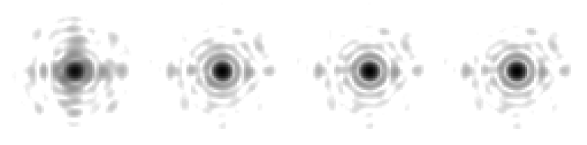
Fig. 9: Focused images obtained on ONERA AO bench (logarithmic scale) corresponding to the 4 first points of Figure 8. The one on the left is the image obtained without any pre-compensation. The last image SR is 93.8%. Conditions are the same as in Figure 6.

We plot on the same figure the ratio between $SR_{im}$ and $SR_{Zern}$. The difference between $SR_{im}$ and $SR_{Zern}$ can be explained by the unestimated high order coefficients (higher than $a_{78}$) and the SR measurement bias due to uncertainty on the system (exact over-sampling factor, background subtraction precision, exact fiber size and shape, see Appendix for more details). This ratio $\frac{SR_{im}}{SR_{Zern}}$ is roughly constant after the first iteration and its value at convergence can be estimated to 99.4% which corresponds to a 8 nm RMS phase error. The different values for the first iteration are explained by the approximation of SR by the coherent energy in $SR_{Zern}$, which is only valid for small phase variance.

We plot in Figure 9 the focused images recorded on the camera without NCPA pre-compensation and after respectively 1, 2 and 3 iterations of the PCL scheme. The correction of low order aberrations allows for the cleaning of the center of the image where two Airy rings are clearly visible with the first one being complete. Around these rings, we observe residual speckles due to the uncompensated higher order aberrations.

6.B Defocus determination

As explained in Section 5, NCPA defocus estimation has to be considered with a particular care since it is biased by uncertainty on the “known aberration” (actually not perfectly known) introduced in the PD method. In order to overcome this bias, two approaches are proposed after the convergence of the pre-compensated scheme. The first one is based on a SR optimization, the second one is a one-shot measurement with an “astigmatism” phase-diversity.

6.B.1 SR optimization

After a few iterations of the PCL (enough to reach the convergence), we modify the pre-compensated $a_{4}$ coefficient in a given range around the estimated coefficient and we measure the corresponding SR. Figure 10 shows the SR evolution with the value of $a_{4}$. The maximum SR is obtained for $a_{4}=34nm$ which is somewhat different from the value given by PD (43nm). The resulting gain in term of SR is around 1%.

Fig. 10: Optimization of the coefficient $a_{4}$, by changing its value before applying the correction slopes. $a_{4}=43nm$ is the value estimated by PD and $a_{4}=34nm$ is the value estimated by the maximum SR. Conditions are the same as in Figure 6 except for the number of compensated Zernike : up to $Z_{36}$.

6.B.2 Astigmatism phase-diversity

An alternative way to perform the NCPA defocus optimization is to use another known aberration between the two images. As explained in the first section, defocalisation is generally used because of its easy implementation. In our case the deformable mirror itself is used to generate the known aberration. Thus any Zernike polynomial can be considered, as long as it is an even radial order (to solve the estimation phase indetermination) and feasible by the DM.

At convergence of the PCL, we acquire a pair of images differing by astigmatism ($Z_{5}$). The PD measurement performed gives coefficients $a_{4}$ to $a_{78}$, with a biased estimation of $a_{5}$ (the previous error due to model uncertainty is now done on $a_{5}$ instead of $a_{4}$) while the coefficient $a_{4}$ is now correctly estimated. The value given for $a_{4}$ by this method is $a_{4}=35nm$ which is fully compatible with the SR optimization of the previous section.

6.C Test of optimized algorithms

Let us now experimentally validate the various PD algorithm modifications proposed in Section 3 (that is non-uniform noise model and phase regularization).

In order to experimentally test these improvements, two different regimes of SNR have been used: high SNR regime as before, $SNR=3\times 10^{4}$ and low SNR regime, $SNR=10^{2}$ obtained with the smallest exposure time while acquiring the pair of images.

Table 2 gathers the various SR values obtained after convergence of the PCL process for the different algorithm modification.

At high SNR, the correction remains extremely good whatever the algorithm configuration. The gain brought by the non-uniform noise model is rather small and the limitation comes from other error terms, especially non-corrected modes. However, there is a slight gain of 0.1% of SR shown in Figure 11 which was predicted by the theory. At low SNR, the gain is much higher, 10% in SR but this is the result of a one-shot test, not a mean gain obtained on a large number of trials.

Fig. 11: Evolution of SR with iteration number. Solid line : the conventional algorithm (uniform noise model). Dotted line : the non-uniform noise model algorithm. The measurements were done at the time for each iteration. Conditions are the same as in Figure 6, except for the used PD algorithm.

The gain brought by the use of the phase regularization term is shown in low SNR regime. At $SNR=10^{2}$, the conventional algorithm without regularization barely estimates the phase. It leads to a poor result after pre-compensation: the saturation plateau remains around 72.1% showing no real improvement on the image. When the regularization term is added, the SR value reaches 91.9%. The NCPA are estimated at almost the same accuracy than in high SNR regime.

As shown in section 3.B, the use of regularization allows the minimization of the noise amplification on the high order estimated modes and enhances the estimation accuracy of the lower orders. This properties will be particularly useful with an infrared camera where the SNR in the image could be limited and when a large number of modes have to be estimated. Note also the substantial gain brought by the use of the non-uniform noise model algorithm when compared to the conventional one and also when coupled to the phase regularization.

Table 2: SR obtained with the different optimized algorithms.

	Conventional	Non-uniform	Phase	Regularization and
	algorithm	noise model	Regularization	non-uniform noise model
Max SR	93.8%	93.9%	93.8%	93.9%
for high SNR
Max SR	72.1%	81.2%	91.9%	92.3%
for low SNR

6.D Number of modes

An additional test has been performed with the PCL. In this test, the conditions are the same than previously, i.e. : 75 Zernike modes are measured by PD. The SNR in the images used by PD is very high (10⁴). The PD algorithm used to perform NCPA measurement is the conventional one. The NCPA $a_{4}$ estimation is unbiased (see Section 6.B). In this test 42 Zernike modes have been compensated, instead of 25.

The corresponding PSF is shown in Figure 12, revealing up to 4 Airy rings. A SR of 98.7% is obtained. Figure 13 presents the measured Zernike coefficients before any compensation and after three iterations of PCL corresponding to Figure 12. A 13 nm total residual error was estimated on the 75 Zernike coefficients, a substantial gain when compared to the result of Figure 7 (24.5 nm). Up to $Z_{45}$, the residual error is 4.5nm, while the higher order contribution remains below than 12.5 nm. We observe that on the first order, the residual error is slightly higher when compared to the results of Section 6.A (only 1nm). As explained in section 4.B, the high order Zernike modes of NCPA are not well fitted by the DM. That induces some coupling effects between the compensated highest order modes (from $Z_{29}$ to $Z_{45}$) and the uncompensated ones (above $Z_{45}$). They induced some aliasing effect on lower modes, slightly decreasing their pre-compensation efficiency. Nevertheless, the gain brought by the partial correction of highest order modes is higher than the loss due to aliasing effects.

Note that these performance were obtained using a Kalman filter in the AO loop as developed for optimized compensation of the turbulence,${}^{\hbox{\immediate{\bf{?}}}}$ and not a simple integrator corrector as for the previous result. This Kalman filter uses the first 130 Zernike modes for the WFS phase regularized estimation, leading to partially overcome the limitations linked to the bad fitting of the high order Zernike by the DM. It was not possible to obtain such a high SR (98.7%) with the integrator in the same conditions.

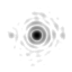
Fig. 12: PSF obtained after three iterations of NCPA pre-compensation. 42 modes are compensated (from $Z_{4}$ to $Z_{45}$), and the exact value of $a_{4}$ has been optimized. SR is 98.7%, $\lambda=632.8nm$.

Fig. 13: Zernike coefficients measured before compensation (dotted line) and after 3 iterations of PCL (Dashed line, corresponding to the PSF shown in the Figure 12). The conditions are the same than in Figure 12.

7 Discussion

We discuss here the gain brought by our new approach for NCPA measurement and compensation on extreme AO systems for extrasolar planet detection. This type of instrument requires very high AO performance in order to directly detect photons coming from very faint companions orbiting their parent star. An example of such an extreme AO system applied to direct exoplanet detection is SAXO ,${}^{\hbox{\immediate{?}}}$ the extreme AO system of SPHERE .${}^{\hbox{\immediate{?}}}$ SPHERE is a 2nd generation VLT instrument considered for first light in 2010. It will allow one to detect hot Jupiter-like planets with the contrast up to $10^{6}$.

Characteristics of SAXO are the following ${}^{\hbox{\immediate{?}}}$ : a 41 by 41 actuator DM and a WFE budget of 80nm after extreme AO correction (90% SR in H band). The specification of SAXO is to compensate for NCPA with at least 100 Zernike modes (goal 200) and to allocate a 8nm WFE on these modes.

The high number of actuators available on the DM allows one to fit the requested number of modes (no fitting problem). Therefore, the only error source is therefore assumed to be a PD estimation error.

According to Figure 5 and to the fact that precision of PD is inversely proportional to SNR in image ,${}^{\hbox{\immediate{?}}}$ a SNR of $10^{4}$ is sufficient to have a precision of $0.4nm^{2}$ on each of the 100 measured Zernike, i.e. a residual WFE of 6nm. This SNR can be achieved by averaging a number of images recorded by the infrared camera. Moreover, this level of residual correction per Zernike mode is fully compatible with the results obtained on our AO Bench (see Figure 6 and 13). The goal of 100 Zernike for compensation and 8nm of WFE after compensation is therefore fully achievable with the PCL and optimized algorithms presented here.

8 Conclusion

We have proposed and validated a new and efficient approach for the measurement and pre-compensation of the NCPA. First, the measurement quality of NCPA has been improved via the optimization of PD algorithm (accurate noise model, phase regularization). Moreover the limitation imposed by model uncertainties during the pre-compensation process has been overcome by the use of a new iterative approach (PCL).

We have experimentally validated this new tool on the ONERA AO bench. Very high SR has been obtained (around 98.7% of SR at 633 nm, that is less than 14nm of residual defects). The residual WFE on corrected modes is less than 4.5nm RMS. We have estimated the residual error on uncorrected aberrations to be less than 12.5nm RMS. Solutions have been proposed to deal with experimental issues (such as defocus uncertainty) of the PD implementation.

The experimental results presented in this paper allow us to be confident in our capability of achieving the challenging performance required for extrasolar planet direct detection. The residual errors obtained on our AO bench for NCPA compensation are fully compatible with the error budget of an extreme AO system like SAXO. Using 100 Zernike in the compensation we should achieve a 8nm residual error, corresponding to 99.9% SR, @1.6$\mu m$.

Appendix A Strehl ratio estimation

A.A Strehl Ratio estimation in focal plan images

A widely used performance estimator in AO is the SR. Its experimental estimation is difficult and requires optimized algorithms able to deal with a number of experimental biases or noises. We propose here an efficient SR measurement procedure. The SR is defined as the ratio of the on-axis value (or tilt free) of the aberrated image $i_{ab}$ on the on-axis value of the aberrations-free image $i_{Airy}$. Several parameters have to be taken into account in order to obtain accurate and unbiased values: the residual background and the noise in the image, the CCD pixel scale, and the size of the calibration source used to calibrate the NCPA.

The SR value can be computed using the following equations:

$$SR_{im}=\frac{i_{ab}(\vec{0})}{i_{Airy}(\vec{0})}=\frac{\int\tilde{i}_{ab}(\vec{f}).d\vec{f}}{\int\tilde{i}_{Airy}(\vec{f}).d\vec{f}}$$ (A.1)

where $\tilde{i}_{ab}$ and $\tilde{i}_{Airy}$ are the optical transfer function (OTF) of the aberrant system and of the aberration-free system respectively ($\tilde{i}$ standing for Fourier Transform of $i$), $\vec{f}$ a position variable in Fourier space. We developed a procedure calculating the SR in the Fourier domain. Considering OTF rather than the PSF for SR estimation presents several advantages which are summarized below, and illustrated in Figure 14.

• First, an analysis of the FT of the aberrated image (OTF) allows a fine subtraction of the residual background which can be estimated from a parabolic fit at the lowest frequencies of the aberrated OTF excluding the zero frequency.

• An important point is the adjustment of the cut-off frequency ($f_{c}=\frac{D}{\lambda}$) in $\tilde{i}_{Airy}$ (value in frequency pixel directly linked to the image pixel scale) to the experimental value in the aberrated OTF. The pixel scale is also used by PD to estimate the phase.

• Actually, all the OTF values for frequencies greater than the cut-off frequency are only noise. An estimation of this level and then a subtraction to the aberrated OTF allow us to refine the SR estimation. In Figure 14, for higher frequencies than $f_{c}$ the aberrated OTF presents a noise plateau at 1.e-3.

• At last the procedure also takes into account the transfer function of the CCD and of the FT of the object, when the last one is partially resolved by the optical system.

Fig. 14: Measured OTF from the image (Dashed line), the OTF corrected for noise and background contributions (solid line), and the adjusted Airy OTF as obtained by the SR measurement procedure (dot-dashed line. The cut-off frequencies are adjusted to be superimposed. The transfer function of the CCD is also given (dotted line).

A.B Errors in Strehl ratio estimation

Practical instrumental limitations degrade the SR estimation accuracy even when using an optimized algorithm as in Section 3. It is important to quantify their influence in order to give error bars on SR values.

A.B.1 Influence of residual background

Let’s first study the influence of a residual uniform background $\delta B$ per pixel on the estimation of the $SR$ in an image $i_{f}$.

Using Equation A.1 we can express the background contribution in the SR computation as follows:

$$SR_{im} = \frac{\left(i_{f}(\vec{0})+\delta B\right)\int{i_{Airy}(\vec{\alpha})d\vec{\alpha}}}{i_{Airy}(\vec{0})\int{\left(i_{f}(\vec{\alpha})+\delta B\right)d\vec{\alpha}}}$$

$$\simeq SR\left(1+\frac{\delta B}{i_{f}(\vec{0})}\right)\left(1-\frac{N^{2}\delta B}{\int{i_{f}(\vec{\alpha})d\vec{\alpha}}}\right)$$

Note that Equation A.B.1 takes into account the required normalization by the total flux in the image ($\int{\left(i_{f}(\vec{\alpha})+\delta B\right)d\vec{\alpha}}$), where the image $i_{f}(\vec{\alpha})$ has $N$x$N$ pixels and $\int{i_{Airy}(\vec{\alpha})d\vec{\alpha}}=1$. Considering that generally $\delta B<<i_{f}(\vec{0})$, a residual background $N^{2}\delta B$ equal to 1% of the total flux in the image modifies the SR value of 1% as well. The residual background in our images after subtraction of the calibrated background and after correction by fitting of the lowest frequencies of the OTF is estimated at $\pm 0.1\%$ of the total flux using images of 128x128 pixels. The SR estimation accuracy is therefore $\pm 0.1\%$.

A.B.2 Influence of an uncertainty on the pixel scale

The pixel scale is a parameter to be experimentally estimated since it greatly depends on components characterization and system implementation. It plays an important role in the NCPA estimation through the PD algorithm. It also impacts the SR estimation quality. Its influence is therefore major on the whole procedure discussed in this paper. In the next section, we emphasize its influence on the SR measurement.

Assuming that the OTF profile for an Airy pattern has a linear shape, a simple computation shows that the relative SR modification $\frac{\delta SR}{SR}$ is directly equal to twice the relative precision $\frac{\delta e}{e}$ on the pixel scale $e$, that is:

$$\frac{\delta SR}{SR}=-2\frac{\delta e}{e}$$ (A.3)

It is clear that knowledge of $e$ is essential to obtain an accurate estimation of SR. Nevertheless, $e$ value doest not evolve with time Therefore the estimation error on SR is constant for all the test. The impact on SR is a bias. In other words, if $e$ value is critical for absolute SR computation, its influence is dramatically reduced when only relative evolution of SR are considered. (Gain brought by a new approach of NCPA pre-compensation for example).

Now the essential question is : “with which accuracy do we know the pixel scale?”. In images taken on different days, the measured cut-off frequency is stable with an uncertainty lower than half a frequency pixel. The random relative error on the pixel scale is 0.4% for 128 frequency pixels. Finally, we used the same measured pixel scale ($e=\lambda/4.1D$) in data processing of all the performed experiments (NCPA measurement and SR estimation). The relative error on SR estimation is therefore a bias of 0.8%. Because $SR\simeq 100\%$, the absolute error on $SR$ is $0.8\%$.

A.B.3 SR accuracy in experimental data

It is now possible to estimate a global accuracy of the SR estimation using the results of Section A.B.1 and A.B.2: $\sigma_{SR}=\sqrt{0.8^{2}+0.1^{2}}\simeq.81\%$. The pixel scale bias is the main contribution to this value.

A.C SR estimated using the measured Zernike coefficients

Another way to estimate $SR$ is to use the residual phase variance $\sigma_{\phi}^{2}$ to compute the coherent energy $e^{\left(-\sigma_{\phi}^{2}\right)}$. The residual phase variance can be directly obtained using the PD estimated Zernike coefficients. We therefore define the approximated SR $SR_{Zern}$ by:

$$SR_{Zern}=\exp\left(-\sum_{k=2}^{N_{max}}a_{k}^{2}\right)$$ (A.4)

where $a_{k}$ stands for the k^th Zernike coefficient. In one hand, this expression of $SR_{Zern}$ is a lower bound for the true SR for relatively large residual phase (low SR). In the other hand, $SR_{Zern}$ is a good approximation of SR for small residual phases (high SR). But it slightly over estimates it since $SR_{Zern}$ only accounts for the $N_{max}$ first Zernike (Equation A.4). Figure 8 shows the image measured SR ($SR_{im}$) and computed one ($SR_{Zern}$). We verify on this figure the behavior described here above.

References

- [1] J.-L. Beuzit, D. Mouillet, C. Moutou, K. Dohlen, P. Puget, T. Fusco, and A. Boccaletti et al.. A planet finder instrument for the vlt. In IAUC 200, Direct Imaging of Exoplanets: Science & Techniques, 2005. Date conférence : October 2005, Nice, France.
- [2] C. Cavarroc, A. Boccaletti, P. Baudoz, T. Fusco, and D. Rouan. Fundamental limitations on Earth-like planet detection with extremely large telescopes. Astron. Astrophys., 447:397–403, February 2006.
- [3] T. Fusco, G. Rousset, J.-F. Sauvage, C. Petit, J.-L. Beuzit, K. Dohlen, D. Mouillet, J. Charton, M. Nicolle, M Kasper, and P. Puget. High order adaptive optics requirements for direct detection of extra-solar planets. application to the sphere instrument. Opt. Express, (17):7515–7534, 2006.
- [4] R. A. Gonsalves. Phase retrieval and diversity in adaptive optics. Optical Engineering, 21(5):829–832, 1982.
- [5] R. G. Paxman, T. J. Schulz, and J. R. Fienup. Joint estimation of object and aberrations by using phase diversity. Journal of the Optical Society of America A, 9(7):1072–1085, 1992.
- [6] L. Meynadier, V. Michau, M.-T. Velluet, J.-M. Conan, L. M. Mugnier, and G. Rousset. Noise propagation in wave-front sensing with phase diversity. Appl. Opt., 38(23):4967–4979, August 1999.
- [7] A. Blanc, L. M. Mugnier, and J. Idier. Marginal estimation of aberrations and image restoration by use of phase diversity. J. Opt. Soc. Am. A, 20(6):1035–1045, 2003.
- [8] G. Rousset, F. Lacombe, P. Puget, N. Hubin, E. Gendron, T. Fusco, R. Arsenault, J. Charton, P. Gigan, P. Kern, A.-M. Lagrange, P.-Y. Madec, D. Mouillet, D. Rabaud, P. Rabou, E. Stadler, and G. Zins. NAOS, the first AO system of the VLT: on sky performance. In Peter L. Wizinowich and Domenico Bonaccini, editors, Adaptive Optical System Technology II, volume 4839, pages 140–149, Bellingham, Washington, 2002. Proc. Soc. Photo-Opt. Instrum. Eng., SPIE.
- [9] M. A. van Dam, D. Le Mignant, and B. A. Macintosh. Performance of the Keck Observatory Adaptive-Optics System. ao, 43:5458–5467, 2004.
- [10] M. Hartung, A. Blanc, T. Fusco, F. Lacombe, L. M. Mugnier, G. Rousset, and R. Lenzen. Calibration of NAOS and CONICA static aberrations. Experimental results. Astron. Astrophys., 399:385–394, 2003.
- [11] A. Blanc, T. Fusco, M. Hartung, L. M. Mugnier, and G. Rousset. Calibration of NAOS and CONICA static aberrations. Application of the phase diversity technique. Astron. Astrophys., 399:373–383, 2003.
- [12] J.-M. Conan, L. M. Mugnier, T. Fusco, V. Michau, and G. Rousset. Myopic deconvolution of adaptive optics images by use of object and point spread function power spectra. Appl. Opt., 37(21):4614–4622, July 1998.
- [13] L. M. Mugnier, T. Fusco, and J.-M. Conan. MISTRAL: a myopic edge-preserving image restoration method, with application to astronomical adaptive-optics-corrected long-exposure images. J. Opt. Soc. Am. A, 21(10):1841–1854, October 2004.
- [14] G. Rousset. Wavefront sensing. In D. Alloin and J.-M. Mariotti, editors, Adaptive Optics for Astronomy, volume 243, pages 115–137, Cargèse, France, 1993. ASI, Kluwer Academic Publisher.
- [15] J. Kolb, E. Marchetti, G. Rousset, and T. Fusco. Calibration of an MCAO system. In Advancements in Adaptive Optics, volume 5490. Proc. Soc. Photo-Opt. Instrum. Eng., SPIE, 2004. Date conférence : June 2004, Glasgow, UK.
- [16] C. Petit, J.-M. Conan, C. Kulcsar, H.-F. Raynaud, T. Fusco, J. Montri, and D. Raboud. First laboratory demonstration of closed-loop kalman based optimal control for vibration filtering and simplified mcao. In L. Ellerbroek, B. and D. Bonaccini Calia, editors, Advances in Adaptive Optics II, volume 6272. Soc. Photo-Opt. Instrum. Eng., 2006.