Estimating Power Spectrum of Sunyaev-Zeldovich Effect from the Cross-Correlation between WMAP and 2MASS

Abstract

We estimate the power spectrum of SZ(Sunyaev-Zel’dovich)-effect-induced temperature fluctuations on sub-degree scales by using the cross correlation between the three-year WMAP maps and 2MASS galaxy distribution. We produced the SZ effect maps by hydrodynamic simulation samples of the $\Lambda$CDM model, and show that the SZ effect temperature fluctuations are highly non-Gaussian. The PDF of the temperature fluctuations has a long tail. More than $70\%$ power of the SZ effect temperature fluctuations attributes to top $\sim 1\%$ wavelet modes (long tail events). On the other hand, the CMB temperature fluctuations basically are Gaussian. Although the mean power of CMB temperature fluctuations on sub-degree scales is much higher than that of SZ effect map, the SZ effect temperature fluctuations associated with top 2MASS clusters is comparable to the power of CMB temperature fluctuations on the same scales. Thus, from noisy WMAP maps, one can have a proper estimation of the SZ effect power at the positions of the top 2MASS clusters. The power spectrum given by these top wavelet modes is useful to constrain the parameter of density fluctuations amplitude $\sigma_{8}$. We find that the power spectrum of these top wavelet modes of SZ effect on sub-degree scales basically is consistent with the simulation maps produced with $\sigma_{8}=0.84$. The simulation samples of $\sigma_{8}=0.74$ show, however, significant deviation from detected SZ power spectrum. It can be ruled out with confidence level 99% if all other cosmological parameters are the same as that given by the three-year WMAP results.

1 Introduction

The thermal Sunyaev-Zel’dovich (SZ) effect is due to the inverse Compton scattering of the cosmic microwave background (CMB) photons by hot electrons. This effect is proportional to the pressure of the electron gases, $p=k_{B}nT$, where $n$ and $T$ being the number density and temperature of electrons. Therefore, SZ effect can be used as a measurement of the hot baryon gases of the universe (e.g. Birkinshaw 1999; Carlstrom et al. 2002). Since clusters are the hosts of high pressure gases, the angular power spectrum of the SZ effect is very sensitive to the amplitude of mass density fluctuations parameter $\sigma_{8}$ (Refregier et al. 2000; Bond et al. 2002). The amplitude of the SZ effect angular power spectrum is found to be proportional to $\sigma_{8}^{7}(\Omega_{b}h)^{2}$ and is almost independent of other cosmological parameters (e.g. Seljak et al. 2001; Komatsu & Seljak 2002). Therefore, the amplitude of the SZ effect power spectrum can be used as an effective constraint on the parameter $\sigma_{8}$. The SZ effect power spectrum on scales of a few arcminutes has been used for this issue (Mason et al.2003; Readhead et al. 2004; Dawson et al. 2006).

Recently released WMAP three-year data (WMAP III) refines most results of cosmological parameters given by the WMAP first year data. They found $\sigma_{8}=0.74\pm 0.05$ (Spergel et al. 2006), which is significantly lower than $\sigma_{8}=0.84\pm 0.04$ of the first year data. The new number of $\sigma_{8}$ is a challenge to the cosmological parameter determined with samples of galaxies and galaxy clusters, most of which yield $\sigma_{8}\simeq 0.9-1$ if the matter content of the universe $\Omega_{m}\leq 0.3$ (Reiprich & Böhringer 2002; Hoekstra et al. 2002; Refregier, et. al. 2002; Van Waerbeke et. al. 2002; Bacon et al. 2003; Bahcall & Bode 2003; Seljak, et al. 2005; Viel & Haehnelt 2006; McCarthy et al. 2006; Cai et al. 2006). This problem motivates us to study the constraint on $\sigma_{8}$ given by the power spectrum of the SZ effect.

We try to extract the information of the SZ effect power spectrum on sub-degree scales from the WMAP III data themselves. At the first glance, it seems to be hopeless to extract such information from noisy WMAP III data, because the power of SZ effect induced temperature fluctuations on sub-degree scales is much less than that of CMB temperature fluctuations (e.g. Cooray et al. 2004). A direct analysis on the WMAP data also shows that the SZ effect contribution to the CMB fluctuations on scale of the first acoustic peak should be less than 2% (Huffenberger et al. 2004; Spergel et al. 2006).

This problem can be solved if considering that the SZ effect map is highly non-Gaussian, while CMB is Gaussian. Although the mean power of the thermal SZ effect on sub-degree scales is no more than $2\%$ of the power of CMB, the SZ temperature fluctuations at local modes associated with clusters are comparable to the CMB temperature fluctuations. Thus, the SZ temperature fluctuations power on sub-degree scales would be detectable from noisy WMAP maps if one can identify such local modes. To implement this detection, we developed a DWT(discrete wavelet transform) algorithm for the power spectrum estimation. The DWT analysis is powerful to pick up weak but non-Gaussian signals from Gaussian background (Donoho 1995).

We will use the cross-correlation between the WMAP III data and 2MASS galaxies. Since the redshift of 2MASS XSC galaxies is up to $z\simeq 0.1$, at which clusters are on angular scales of sub-degree. Moreover, the thermal SZ effect on angular scales of clusters has been significantly identified with the 2nd and 4th order cross-correlations between the first year WMAP data and 2MASS XSC galaxies(Afshordi et al. 2004, 2005; Myers et al. 2004; Cao et al. 2006). The WMAP-2MASS cross-correlation would be effective to extract the SZ power on sub-degree scales from the WMAP III maps.

The paper is organized as follow. In §2, we analyze the non-Gaussian features of the SZ effect maps generated with cosmological hydrodynamic simulation. §3 describes the identification of the SZ effect of 2MASS clusters from the WMAP-2MASS cross correlation with the wavelet modes. §4 first describes the algorithm of estimating the SZ power spectrum from the WMAP III maps, and then presents the result of the SZ effect constraint on $\sigma_{8}$. The discussion and conclusion are given in §5.

2 The power spectrum of SZ effect fluctuations

2.1 Maps of SZ effect

To develop the method of estimating power spectrum, we first study the statistical properties of the SZ effect temperature fluctuations. We produce the SZ effect maps with the WIGEON (Weno for Intergalactic medium and Galaxy Evolution and formatiON) code, which is a cosmological hydrodynamic $N$-body code based on the Weighted Essentially Non-Oscillatory (WENO) algorithm (Harten et al. 1986; Liu et al. 1994; Jiang & Shu 1996; Shu 1998; Fedkiw, Sapiro & Shu 2003; Shu 2003). The details of this code can be found at Feng et al. (2004). Some WIGEON samples have already been used in cosmological studies (e.g. He et al. 2004, 2006; Zhang et al. 2006; Liu et al. 2006).

The samples are simulated in a 100 $h^{-1}$ Mpc cubic box with 512³ meshes for gas, and equal number of particles for dark matter. We use the standard $\Lambda$CDM model, which is specified by the matter density parameter $\Omega_{\rm m}=0.27$, baryon density parameter $\Omega_{\rm b}=0.044$, cosmological constant $\Omega_{\Lambda}=0.73$, Hubble constant $h=0.71$. In order to test the effect of the amplitude of density fluctuations, we produce two samples with $\sigma_{8}=0.74$ and 0.84, respectively. The ratio of specific heats is $\gamma=5/3$. The transfer function is calculated using CMBFAST (Seljak & Zaldarriaga 1996). In order to correct the underestimate of rare massive galaxy clusters due to the finite box size, the initial conditions are generated by sampling a convolved power spectrum following the method of Pen (1997) and Sirko (2006), which accurately model the real-space statistics, such as $\sigma_{8}$.

The atomic processes including ionization, cooling and heating are modeled as the method in Theuns et al. (1998). We take a primordial composition of H and He ($X$=0.76, $Y$=0.24) and use an ionizing background model of Haardt & Madau (1996). Star formation and their feedback due to supernova explosions and AGN activities were not taken into account.

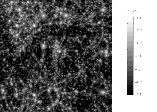
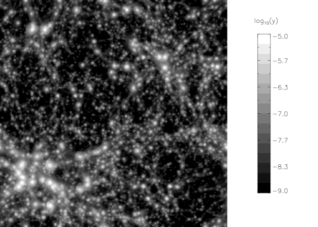
Figure 1: The SZ effect Compton parameter $y$ maps of simulation samples with redshift $z\leq 0.1$ and $\sigma_{8}=0.74$(top) and $\sigma_{8}=0.84$(bottom).

Since the redshift of 2MASS galaxies is up to 0.1, we produce the SZ maps by integrating the pressure of gas from $z=0$ to 0.1. The simulation data is stored for every redshifts corresponding to comoving distance $n\times$100$h^{-1}$Mpc, $n$ being integral. Three simulation boxes are stacked together and integrated along different angular direction to compose a SZ map. Two 2-D maps of the Compton parameter $y$ for $\sigma_{8}=0.74$ and 0.84 are shown in Figure 1. Both maps have a size of $19.1^{\circ}\times 19.1^{\circ}$, with resolution of 512$\times$512. We produce 40 independent maps. The total area, $40\times(19.1^{\circ})^{2}$, is comparable with the area of 2MASS data we used (§3.1).

Figure 2 gives the angular power spectrum for two samples with $\sigma_{8}=0.74$ and 0.84, respectively. We see that the amplitude of the power spectrum is significantly dependent on $\sigma_{8}$. Comparing Figure 2 with other simulations (e.g. Refregier et al. 2000; Seljak et al. 2001; Komatsu & Seljak 2002), our result shows about the same power as others on scales equal to and larger than $0^{\circ}.5$, while it is much lower than others on scales $\ll 0^{\circ}.5$. This is expected, as the power on scales less than $0^{\circ}.5$ mainly comes from clusters with redshift $>0.1$. If considering all the contribution from $z=6$, our simulation samples show the same behavior as others, i.e., declining around $0^{\circ}.1$.

2.2 The DWT power spectrum of SZ effect map

As shown by Figure 1, the value of $y$ is very small in most space, while high value of $y$ appears only in small and localized areas. One can then take the advantage of DWT analysis to describe the field $y({\bf x})$ (${\bf x}=(x_{1},x_{2})$) with DWT decomposition. The DWT variables of a map $y(x_{1},x_{2})$ in the area of $0\leq x_{1}\leq L_{1}$ and $0\leq x_{2}\leq L_{2}$ are given by the decompositions of scaling functions $\phi_{\bf j,l}({\bf x})$ and wavelet functions $\psi_{\bf j,l}({\bf x})$. We use Daubechies 4 wavelet (Daubechies (1992), Fang & Thews (1998). The functions $\phi_{\bf j,l}({\bf x})$ and $\psi_{\bf j,l}({\bf x})$ can also be found in Yang et al. (2001).

Briefly, The DWT scaling function, $\phi_{\bf j,l}({\bf x})$, is a window function for cells (modes) in the area $L_{1}l_{1}/2^{j_{1}}<x_{1}<L_{1}(l_{1}+1)/2^{j_{1}}$ and $L_{2}l_{2}/2^{j_{2}}<x_{2}<L_{2}(l_{2}+1)/2^{j_{2}}$. The scale index ${\bf j}=(j_{1},j_{2})$, $j_{1}$ and $j_{2}$ can be any positive integer. The position index ${\bf l}=(l_{1},l_{2})$, $l_{1}$ and $l_{2}$ can be 0, 1… $2^{j_{1}}-1$, and 0, 1… $2^{j_{2}}-1$, respectively. On the other hand, the wavelet function is admissible, satisfying $\int\psi_{\bf j,l}({\bf x})d{\bf x}=0$.

For the field $y({\bf x})$, the DWT variables are

$$y_{\bf j,l}=\frac{1}{\int\phi_{\bf j,l}({\bf x})d{\bf x}}\int y({\bf x})\phi_{\bf j,l}({\bf x})d{\bf x},$$ (1)

$$\tilde{\epsilon}^{y}_{\bf j,l}=\int y({\bf x})\psi_{\bf j,l}({\bf x})d{\bf x},$$ (2)

Since $\phi_{\bf j,l}({\bf x})$ is a window function of cell $\bf(j,l)$, $y_{\bf j,l}$ is the mean of $y(\bf x)$ in cell $\bf(j,l)$. Because $\psi_{\bf j,l}({\bf x})$ is admissible, $\tilde{\epsilon}^{y}_{\bf j,l}$ measures the fluctuation of field $y({\bf x})$ with respect to the mean, $y_{\bf j,l}$, in the mode $({\bf j,l})$. For a given ${\bf j}$, the mean of $\langle\tilde{\epsilon}^{y}_{\bf j,l}\rangle$ over all modes is zero (Fang & Thews 1998). Since the basis $\psi_{\bf j,l}$ are orthogonal and complete, the DWT variables of the field $y({\bf x})$ do not lost information and cause false correlations.

With the DWT variables, the power spectrum of the 2-D field $y({\bf x})$ can be measured as (Pando & Fang 1998; Fang & Feng 2000):

$$P_{\bf j}=\langle|\tilde{\epsilon}_{\bf j,l}|^{2}\rangle\equiv\frac{1}{2^{j_{1}+j_{2}}}\sum_{l_{1}=0;l_{2}=0}^{2^{j_{1}}-1;2^{j_{2}}-1}|\tilde{\epsilon}^{y}_{j_{1},j_{2};l_{1},l_{2}}|^{2},$$ (3)

$|\tilde{\epsilon}^{y}_{j_{1},j_{2};l_{1},l_{2}}|^{2}$ is the power at mode $({\bf j,l})=(j_{1},j_{2};l_{1},l_{2})$. Therefore, the DWT power spectrum $P_{\bf j}$ actually is the mean of local powers $|\tilde{\epsilon}_{\bf j,l}|^{2}$ over all $2^{j_{1}+j_{2}}$ modes on scale ${\bf j}$. It has been shown that the DWT power spectrum can be expressed by the Fourier power spectrum as (Fang & Feng 2000; He et al. 2005a):

$$P_{\bf j}=\frac{1}{2^{j_{1}+j_{2}}}\sum_{n_{1}=-\infty}^{\infty}\sum_{n_{2}=-\infty}^{\infty}|\hat{\psi}(n_{1}/2^{j_{1}})\hat{\psi}(n_{2}/2^{j_{2}})|^{2}P(n_{1},n_{2}),$$ (4)

where $\hat{\psi}(n)$ is the Fourier transform of the basic wavelet $\psi(x)$. Because we have the normalized relation $\sum_{n_{1},n_{2}}|\hat{\psi}(n_{1}/2^{j_{1}})\hat{\psi}(n_{2}/2^{j_{2}})|^{2}/2^{j_{1}+j_{2}}=1$, the DWT power spectrum $P_{\bf j}$ is equal to the Fourier power spectrum banded on scales around $(L_{1}L_{2}/2^{j_{1}+j_{2}})^{1/2}$. Figure 3 shows both the angular power spectrum $C_{l}$ and DWT power spectrum $P_{\bf j}$ for the simulation samples. The angular scale of $j$ is $19.1/2^{j}$ degree, and therefore, $l\simeq 9.4\times 2^{j}$. Figure 3 shows that DWT power spectrum is the same as the angular power spectrum $C_{l}$. We will use the DWT analysis on angular scales of sub-degree, on which the effect of spherical surface is not significant.

2.3 Non-Gaussianity of SZ effect map

The DWT power spectrum can effectively detect the non-Gaussian feature of a field (Jamkhedkar et al. 2003). Taking this advantage, one can reveal the non-Gaussianity of the SZ effect field $y({\bf x})$ with the DWT power spectrum of the SZ field $y({\bf x})$ defined as

$$P^{\rm{top}}_{\bf j}=\frac{1}{2^{j_{1}+j_{2}}}\sum_{\rm{top}}|\tilde{\epsilon}_{j_{1},j_{2};l_{1},l_{2}}|^{2},$$ (5)

where summation of “top” goes over only modes having high values $|\tilde{\epsilon}_{j_{1},j_{2};l_{1},l_{2}}|^{2}$ among the $2^{j_{1}+j_{2}}$ modes for a given ${\bf j}$. In Figure 4, we plot the $P_{\bf j}$ and $P^{\rm{top}}_{\bf j}$ of the simulation samples, in which top power spectrum, $P^{\rm{top}}_{\bf j}$, is given by top 1%, 0.3%, 0.1% among the $2^{j_{1}+j_{2}}$ modes. We see that all the power spectra $P^{\rm{top}}_{\bf j}$ are close to $P_{\bf j}$. For samples with $\sigma_{8}=0.84$, there is more than $70\%$, $50\%$, $35\%$ power attributes from top 1%, 0.3%, 0.1% modes, respectively. That is, the power $|\tilde{\epsilon}^{\rm{top}}_{\bf j,l}|^{2}$ of each mode among the top 1% modes should be as high as about 70 times of the mean $\langle{|\tilde{\epsilon}_{\bf j,l}|^{2}}\rangle=P_{\bf j}$. These results show that the field $y({\bf x})$ is highly non-Gaussian. From Figure 4, one can see that for sample with $\sigma_{8}=0.74$, all the power spectra $P^{\rm{top}}_{\bf j}$ of top 1%, 0.3%, 0.1% are less close to $P_{\bf j}$. This is because the clustering of $\sigma_{8}=0.84$ sample is stronger than that of $\sigma_{8}=0.74$.

Because $\langle\tilde{\epsilon}_{\bf j,l}\rangle=0$, the value of $\langle{|\tilde{\epsilon}_{\bf j,l}|^{2}}\rangle^{1/2}$ actually is the standard deviation($\sigma$) of the probability distribution function (PDF) of $\tilde{\epsilon}_{\bf j,l}$. Thus, the events of 70$\langle{|\tilde{\epsilon}_{\bf j,l}|^{2}}\rangle$ actually are $\sim$ 8$\sigma$ events. All the top 1% wavelet modes are 8$\sigma$ events. All the top 0.3% and 0.1% modes correspond, respectively, to $\sim 170$$\langle{|\tilde{\epsilon}_{\bf j,l}|^{2}}\rangle$, and $\sim 350$$\langle{|\tilde{\epsilon}_{\bf j,l}|^{2}}\rangle$, or 13 $\sigma$ and 19 $\sigma$ events. For a Gaussian field, the 10 $\sigma$ events should be no more than $10^{-23}$. Therefore, the PDF of $\tilde{\epsilon}_{\bf j,l}$ has a very long tail. In other words, a significant part of the SZ effect DWT power spectrum is given by the long tail events. These long tail events make the SZ effect on sub-degree scales to be detectable. Although the mean of SZ power $\tilde{\epsilon}_{\bf j,l}$ is less than about 2% of the power of CMB, for long tail events, the SZ power is comparable with that of CMB.

One can estimate the power spectrum of SZ effect temperature fluctuations with the top modes (long tail event) of $\tilde{\epsilon}_{\bf j,l}$. For observed maps, however, not all the top modes of $\tilde{\epsilon}_{\bf j,l}$ are given by SZ effect. To reduce this uncertainty, we add a condition that the useful modes $({\bf j,l})$ for top $\tilde{\epsilon}_{\bf j,l}$ should also be the modes significantly showing SZ effect by the WMAP-2MASS cross correlation. It is equal to assume that the power of SZ effect temperature fluctuations mainly comes from clusters (Komatsu & Kitayama 1999; Komatsu & Seljak 2002). We check this assumption with the relation between variables $y_{\bf j,l}$ and $\tilde{\epsilon}_{\bf j,l}$. We found that the top modes of $|\tilde{\epsilon}_{\bf j,l}|$ are largely coincident with the top modes of the Compton parameter $y_{\bf j,l}$. For sample of $\sigma_{8}=0.84$, $84\%$ top modes of $y_{\bf j,l}$ on the angular scale of $0^{\circ}.5$ are coincident with the top modes of $|\tilde{\epsilon}_{\bf j,l}|$ on the same scale. This result indicates that modes with high $y_{\bf j,l}$ generally are also the modes of high local power of SZ effect temperature fluctuations. High $y_{\bf j,l}$ generally is related to clusters.

The fact that the coincidence between top $y_{\bf j,l}$ and top $\tilde{\epsilon}_{\bf j,l}$ is not 100% is due partially to the so-called warm-hot intergalactic medium (WHIM) (Dave et al 2001; He et al. 2004, 2005b). It shows that a significant fraction of hot baryon gases ($T>10^{5}$) are not located in collapsed structures with high density contrast $\rho/\bar{\rho}>100$, but in the areas with a median overdensity $10<\rho/\bar{\rho}<30$. The WHIM is also the source of SZ effect. Nevertheless, the major part of top modes of $|\tilde{\epsilon}_{\bf j,l}|$ is associated with clusters. Therefore, a proper method to estimate the SZ power spectrum would be to identify the modes with top numbers of both $y_{\bf j,l}$ and $|\tilde{\epsilon}_{\bf j,l}|$. The details of this method will be given in the following two sections.

3 SZ effect identified from WMAP-2MASS correlation

3.1 Data

The data of galaxies in the 2MASS extended source catalog (XSC, Jarrett et al. 2000) used for cross-correlation analysis is the same as Guo et al. (2004) and Cao et al. (2006). That is, we use galaxies of ${\rm K\_m\_k20fe}$, which measures the magnitude inside a elliptical isophote with surface brightness of 20 mag ${\rm arcsec^{-2}}$ in $K_{s}$-band. There are approximately 1.6 million extended objects with $K_{s}<14.3$. To avoid the contaminant of stars, we use a latitude cut of $|b|>10^{\circ}$. We also removed a small number of bright ($K_{s}<9$) sources by the parameters of the XSC confusion flag (${\rm cc\_flag}$) and visual verification score for source (${\rm vc}$). To eliminate duplicate sources and have a uniform sample, we use ${\rm use\_src=1}$ and ${\rm dup\_src=0}$ . We also use a cut of $10.0<K_{s}<14.0$ to ensure the sample is complete greater than $90\%$. This sample contains 987,125 galaxies with redshift up to $z\sim 0.1$.

For the CMB temperature fluctuations, we use the full resolution coadded 3 year sky map (Hinshaw et al. 2006) for $W$ band. The maps have had the ILC(Internal Linear Combination) estimate of the CMB signal to highlight the foreground emissions(Hinshaw et al. 2006). We also use the three annual maps to construct three difference maps between the 1st and 2nd, 2nd and 3rd, 3rd and 1st year, which are useful to check statistical significance.

As in Cao et al. (2006), we subject both the 2MASS and WMAP maps to an equal-area projection. We then have 2-D maps of galaxy number density, $n({\bf x})$, and CMB temperature fluctuations, $\Delta T({\bf x})$ with coordinate ${\bf x}=(x_{1},x_{2})$. As has been shown, the equal-area projection will not affect statistical analysis on sub-degree scales, but helpful for using the DWT method. We analyze the cross correlation between $n({\bf x})$ and $\Delta T({\bf x})$ in two $123^{\circ}.88\times 123^{\circ}.88$ areas, which are, respectively, in the northern and southern sky. The 2MASS XSC galaxies are resolved to 10 arcsec. The beam size of WMAP $W$ band map is $0^{\circ}.22$, while the scale of galaxy clusters at the median redshift of the 2MASS samples is $0^{\circ}.5$.

In order to apply the method of DWT power spectrum (§2.2), we also use the DWT variables to describe the maps $n({\bf x})$ and $\Delta T({\bf x})$. They are wavelet variables $\tilde{\epsilon}^{g}_{\bf j,l}=\int n({\bf x})\psi_{\bf j,l}({\bf x})d{\bf x}$, $\tilde{\epsilon}^{T}_{\bf j,l}=\int\Delta T({\bf x})\psi_{\bf j,l}({\bf x})d{\bf x}$, and scaling function variables $n_{\bf j,l}=\int n({\bf x})\phi_{\bf j,l}({\bf x})d{\bf x}/\int\phi_{\bf j,l}({\bf x})d{\bf x}$, $\Delta T_{\bf j,l}=\int\Delta T({\bf x})\phi_{\bf j,l}({\bf x})d{\bf x}/\int\phi_{\bf j,l}({\bf x})d{\bf x}$. The mode $({\bf j,l})$ occupy a area of $123^{\circ}.88/2^{j_{1}}\times 123^{\circ}.88/2^{j_{2}}$ at position around $[l_{1}(123^{\circ}.88)/2^{j_{1}},l_{2}123^{\circ}.88)/2^{j_{1}}]$. The angular distance between modes ${\bf l}$ and ${\bf l^{\prime}}$ at scale $j$ is given by $\theta=123.88^{\circ}|{\bf l-l^{\prime}}|/2^{j}$.

The variables $\tilde{\epsilon}^{T}_{\bf j,l}$ and $\tilde{\epsilon}^{g}_{\bf j,l}$ describe, respectively, the fluctuations of the CMB temperature and galaxy number density in the mode $({\bf j,l})$, while the variables $\Delta T_{\bf j,l}$ and $n_{\bf j,l}$ describe, respectively, the mean temperature and the mean number density of galaxies in the mode $({\bf j,l})$. Therefore, $n_{\bf j,l}$ and $\Delta T_{\bf j,l}$ can be seen as the maps of galaxies and CMB temperature functions smoothed on scale ${\bf j}$.

3.2 DWT clusters

We picked up top clusters on scale ${\bf j}$ by the top members of $n_{\bf j,l}$. These clusters are called DWT clusters. The details of $n_{\bf j,l}$ identification of clusters have been studied with simulation and real samples (Xu et al. 1999, 2000). It showed that the clusters identified by DWT $n_{\bf j,l}$ are statistically the same as the clusters identified by the friend-of-friend method if the mean size of the friend-of-friend identified clusters is the same as DWT clusters. The clusters identified by the friend-of-friend method usually have very irregular shapes (Jing & Fang 1994) and are inconvenient to estimate the statistical significance of the cross correlation. On the other hand, the DWT variables of 2MASS galaxies $n_{\bf j,l}$ and WMAP map $\Delta T_{j,l}$ are in the same cell, the statistical significance of the $n_{\bf j,l}$-$\Delta T_{\bf j,l}$ cross correlation is unambiguous. Scaling functions are orthogonal with each other, different DWT clusters consist of different galaxies. This is also necessary for statistical analysis which we will take below. With this method, we identify top clusters on scales ${\bf j}=(8,8)$, corresponding to scale $\simeq 1.8$ h^-1 Mpc of the 2MASS samples.

3.3 Thermal SZ effect of 2MASS clusters

The SZ effect of 2MASS galaxies can be measured with the cross-correlation between the WMAP and 2MASS clusters defined as Cao et al.(2006):

$$\Delta T^{\rm wmap-2mass}(|{\bf l-l^{\prime}}|)=\langle C_{\bf j,l}\Delta T_{\bf j^{\prime},l^{\prime}}\rangle,$$ (6)

where the variable $C_{\bf j,l}$ is given by:

$$C_{\bf j,l}=\left\{\begin{array}[]{ll}1&{\rm if\ ({\bf j,l})\ is\ a\ cell\ of\ identified\ clusters},\\ 0&{\rm otherwise}.\end{array}\right.$$ (7)

The average $\langle...\rangle$ covers all the DWT clusters on scale ${\bf j}$. Therefore, $\Delta T^{\rm wmap-2mass}(|{\bf l-l^{\prime}}|)$ measures the mean of the CMB temperature fluctuations on a distance $|{\bf l-l^{\prime}}|$ from identified DWT clusters of 2MASS data. When $|{\bf l-l^{\prime}}|\gg 1$, $\Delta T^{\rm wmap-2mass}(|{\bf l-l^{\prime}}|)$ actually is the mean of $\Delta T$ on a large area, and therefore, it should approach to zero. Figure 5 presents the cross correlation $\Delta T^{\rm wmap-2mass}(|{\bf l-l^{\prime}}|)$ between top 100 ${\bf j}=(8,8)$ DWT clusters and WMAP map, in which the scales ${\bf j^{\prime}}$ of $\Delta T_{\bf j^{\prime},l^{\prime}}$ are taken to be ${\bf j^{\prime}}=(8,8)$, ${\bf j^{\prime}}=(8,7)$, and ${\bf j^{\prime}}=(7,7)$ from top to bottom. In all case $\Delta T_{\bf j^{\prime},l^{\prime}}$ is from the full resolution coadded 3 year WMAP map of $W$ band. The error bars are given by the 1-$\sigma$ standard deviation of the 100 CMB simulations.

Figure 5 shows typical anti-correlation of SZ effect. At the position of DWT clusters, i.e. $|\bf l-\bf l^{\prime}|=0$, the mean of temperature change $\Delta T_{\bf j^{\prime},l^{\prime}}$ is always negative, which is expected from the thermal SZ effect on $W$ band. For ${\bf j^{\prime}}=(8,8)$, $\Delta T^{\rm wmap-2mass}(|{\bf l-l^{\prime}}|=0)\simeq-25\pm 15$ $\mu$K, while for ${\bf j^{\prime}}=(8,7)$ and ${\bf j^{\prime}}=(7,7)$, the temperature decreases are $-20\pm 16$ $\mu$K and $-18\pm 14$ $\mu$K respectively. These results are consistent with that given by cross-correlation of the first year WMAP map and 2MASS galaxies (Myers et al. 2004; Hernández-Monteagudo et al. 2004; Cao et al. 2006).

To further check the SZ signals, we calculate the cross-correlation of eq.(6) by using the maps given by the difference between the 1st and 2nd, 2nd and 3rd, 3rd and 1st year. The results are shown in Figure 6. All the anti-correlations shown in Figures 5 completely disappear in Figure 6. It confirms that the temperature decreases at the positions of the DWT clusters in the three annual maps are about the same and not due to noise.

To view the clusters richness dependence, Figure 7 plots $\Delta T^{\rm wmap-2mass}(|{\bf l-l^{\prime}}|=0)$ against the number of top clusters, $n$. As expected, the higher the richness, the stronger the SZ effect. $\Delta T^{\rm wmap-2mass}(|{\bf l-l^{\prime}}|=0)$ rapidly decreases with the number of top clusters, and approaches to the noise level at $n>300$. We should, however, point out that the positive correlation between the clusters richness and SZ effect is statistical. That is, the order of clusters richness is not, one-by-one, corresponding to the order of the amount of SZ effect temperature decrease. Consequently, the relation of richness-SZ effect in the range $n<100$ is not very stable. When $n\geq 100$, the relation of richness-SZ effect, as shown in Figure 6 is very stable. Therefore, in all the statistics below, the number of top clusters should be $>100$.

In the DWT analysis, wavelet modes are orthogonal from each other. Therefore, the area fraction of top 300 ${\bf j}=(8,8)$ DWT clusters is $300/(2\times 256^{2})=0.23\%$. As shown in §2, the mean power of SZ effect of top 0.3% modes would be 170 times higher than mean power of total mode. On the other hand, on sub-degree scales, the CMB power is higher than the SZ effect power by a factor $\sim 10^{2}$. Therefore, we can expect that the mean of SZ temperature decreases of the top 0.3% modes should be larger than the CMB temperature fluctuations by a factor $\sim\sqrt{170/100}\simeq 1.3$. Figure 8 plots the richness-dependence of the S/N ratio, i.e. the ratio between SZ effect temperature decrease and the $1-\sigma$ error bar shown in Figure 7. Since the error bar of Figure 7 is given by the simulation of CMB temperature fluctuations, and therefore, it actually is to measure the the CMB temperature fluctuations. We see from figure 8 that the S/N ratio is about 1.3 - 1.6. This result is consistent with the estimation mentioned above.

4 Estimation of DWT power spectrum of SZ effect

4.1 Method

The observed CMB temperature fluctuations are given by:

$$\Delta T({\bf x})=\Delta T^{\rm cmb}({\bf x})+\Delta T^{\rm sz}({\bf x})+\Delta T^{\rm second}({\bf x}),$$ (8)

where $\Delta T^{\rm cmb}({\bf n})$ is the primeval temperature fluctuations, $\Delta T^{\rm sz}({\bf x})$ is the SZ effect and $\Delta T^{\rm second}({\bf n})$ is due to secondary effects other than the SZ effect, such as the ISW effect and radio point sources. Since the random fields $\Delta T^{\rm cmb}({\bf x})$, $\Delta T^{\rm sz}({\bf x})$ and $\Delta T^{\rm second}({\bf x})$ basically are uncorrelated from each other, the DWT power spectrum, $P_{\bf j}$, of the observed $\Delta T({\bf x})$ consists of three terms as:

$$P_{\bf j}=P^{\rm cmb}_{\bf j}+P^{\rm sz}_{\bf j}+P^{\rm second}_{\bf j},$$ (9)

where

$$P^{\rm cmb,sz,second}_{\bf j}=\frac{1}{2^{j_{1}+j_{2}}}\sum_{l_{1}=0;l_{2}=0}^{2^{j_{1}}-1;2^{j_{2}}-1}\left|\tilde{\epsilon}^{\rm cmb,sz,second}_{j_{1},j_{2};l_{1},l_{2}}\right|^{2}.$$ (10)

Since $P^{\rm cmb}_{\bf j}$ is about $10^{2}$ times larger than $P^{\rm sz}_{\bf j}$ on angular scale of $\simeq 0^{\circ}.5$, one cannot extract $P^{\rm sz}_{\bf j}$ from noisy map $\Delta T({\bf x})$ if the field $\Delta T^{\rm sz}({\bf x})$ is Gaussian. As shown in §2, the SZ effect DWT power spectrum is largely given by the top modes. The local power of the top DWT modes can be as large as $10^{2}$ times of their average. Therefore, the SZ effect local power of the top modes is comparable to $P^{\rm cmb}_{\bf j}$. On the other hand, the primeval temperature fluctuations $\Delta T^{\rm cmb}({\bf x})$ are Gaussian, and the PDF of local temperature fluctuations $\tilde{\epsilon}^{T}_{\bf j,l}$ is Gaussian with zero mean and standard deviation $(P^{\rm cmb}_{\bf j})^{1/2}$. The primeval temperature fluctuations map does not have the modes with very high local power. Thus, the local power of modes associated with top clusters would be measurable from the noisy map of $\Delta T({\bf x})$.

The measurability of power of top modes can be further tested as follows. Subjecting eq.(8) to a wavelet transform, we have:

$$\tilde{\epsilon}_{\bf j,l}=\tilde{\epsilon}^{\rm cmb}_{\bf j,l}+\tilde{\epsilon}^{\rm sz}_{\bf j,l}+\tilde{\epsilon}^{\rm second}_{\bf j,l},$$ (11)

For most modes $({\bf j,l})$ on scales of clusters, $|\tilde{\epsilon}^{\rm cmb}_{\bf j,l}|$ is much larger than $|\tilde{\epsilon}^{\rm sz}_{\bf j,l}|$, and therefore, the latter is negligible. But for modes corresponding to the top clusters, $|\tilde{\epsilon}^{\rm sz}_{\bf j,l}|$ would be comparable to $|\tilde{\epsilon}^{\rm cmb}_{\bf j,l}|$. On these modes, the term $|\tilde{\epsilon}^{\rm second}_{\bf j,l}|$ is also negligible, as statistically the positions of secondary effect are not coincident to top clusters. Thus, on these modes, we have:

$$|\tilde{\epsilon}_{\bf j,l}|^{2}=|\tilde{\epsilon}^{\rm cmb}_{\bf j,l}|^{2}+|\tilde{\epsilon}^{\rm sz}_{\bf j,l}|^{2},$$ (12)

and therefore,

$$\frac{1}{N_{\rm top}}\sum_{\rm top}|\tilde{\epsilon}^{\rm sz}_{\bf j,l}|^{2}=\frac{1}{N_{\rm top}}\sum_{\rm top}|\tilde{\epsilon}_{\bf j,l}|^{2}-\frac{1}{N_{\rm top}}\sum_{\rm top}|\tilde{\epsilon}^{\rm cmb}_{\bf j,l}|^{2},$$ (13)

where the summation “top” is over modes with top $\tilde{\epsilon}_{\bf j,l}$ and also the top DWT clusters. $N_{\rm top}$ is the number of top modes. Because CMB field is statistically isotropic (uniform), Gaussian and uncorrelated with 2MASS data, the average of the primeval temperature fluctuations power $|\tilde{\epsilon}^{\rm cmb}_{\bf j,l}|^{2}$ done by $(1/N_{\rm top})\sum_{\rm top}$ should be about the same as the average over all modes. We have then:

$$\sum_{\rm top}|\tilde{\epsilon}^{\rm cmb}_{\bf j,l}|^{2}\simeq N_{\rm top}\langle|\tilde{\epsilon}_{\bf j,l}|^{2}\rangle,$$ (14)

where $\langle|\tilde{\epsilon}_{\bf j,l}|^{2}\rangle$ is the mean of $|\tilde{\epsilon}_{\bf j,l}|^{2}$ over all modes on scale ${\bf j}$. Thus, considering $|\tilde{\epsilon}^{\rm sz}_{\bf j,l}|^{2}>0$, eq.(13) yields:

$$\frac{1}{N_{\rm top}}\sum_{\rm top}|\tilde{\epsilon}_{\bf j,l}|^{2}>\langle|\tilde{\epsilon}_{\bf j,l}|^{2}\rangle,$$ (15)

Eq.(15) requires that the mean local power over modes at top clusters should be larger than the mean on all modes.

We test Eq.(15) by the cross correlation defined similar to eq.(6):

$$\Upsilon_{\bf j^{\prime}}(|{\bf l-l^{\prime}}|)=\frac{\langle C_{\bf j,l}|\tilde{\epsilon}_{\bf j^{\prime},l^{\prime}}|^{2}\rangle}{\langle|\tilde{\epsilon}_{\bf j^{\prime},l^{\prime}}|^{2}\rangle},$$ (16)

where $C_{\bf j,l}$ is given by eq.(7). The numerator on the r.h.s. of eq.(16) is to measure the mean local power of CMB temperature fluctuations over the modes of DWT clusters on scale ${\bf j^{\prime}}$. The denominator of eq.(16) is for normalization. The inequality in eq.(15) requires $\Upsilon_{\bf j^{\prime}}(|{\bf l-l^{\prime}}|)>1$ at $|\bf l-\bf l^{\prime}|=0$, i.e. the local power of the modes, which shows significant SZ temperature decrease, should also show power larger than the mean $\langle|\tilde{\epsilon}_{\bf j^{\prime},l^{\prime}}|^{2}\rangle$ over the whole sky. The result of $\Upsilon_{\bf j^{\prime}}(|{\bf l-l^{\prime}}|)$ is plotted in Figure 9, in which the scale ${\bf j^{\prime}}$ of local power $|\tilde{\epsilon}_{\bf j^{\prime},l^{\prime}}|^{2}$ is taken to be ${\bf j^{\prime}}=(8,8)$, ${\bf j^{\prime}}=(8,7)$ and ${\bf j^{\prime}}=(7,7)$. For each scale, we count 0.11% modes with top $|\tilde{\epsilon}_{\bf j^{\prime},l^{\prime}}|^{2}$, and all the counted modes are located in the positions of the 300 top 2MASS clusters, corresponding to 150, 75, and 38 top modes of the scales ${\bf j^{\prime}}=(8,8)$, ${\bf j^{\prime}}=(8,7)$ and ${\bf j^{\prime}}=(7,7)$. Figure 9 shows that all the mean powers of CMB temperature fluctuations on the three scales are significantly larger than the mean $\langle|\tilde{\epsilon}_{\bf j^{\prime},l^{\prime}}|^{2}\rangle$. This power excess is due to the SZ effect of the 2MASS clusters, which are larger than the noise of WMAP III data.

4.2 Results

With these preparation, we can estimate the SZ effect power spectrum given by modes associated with the top DWT clusters of 2MASS galaxies. It is,

$$P^{\rm top}_{\bf j}=\frac{1}{2^{j_{1}+j_{2}}}\sum_{\rm top}|\tilde{\epsilon}^{\rm sz}_{\bf j,l}|^{2},$$ (17)

where the “top” is taken the same modes as shown in Figure 9. Using eqs.(13) and (14), eq.(17) gives,

$$P^{\rm top}_{\bf j}\simeq\frac{1}{2^{j_{1}+j_{2}}}\left[\sum_{\rm top}|\tilde{\epsilon}_{\bf j,l}|^{2}-N_{\rm top}\langle|\tilde{\epsilon}_{\bf j,l}|^{2}\rangle\right].$$ (18)

This is the basic formula of extracting the SZ temperature fluctuations power spectrum of 2MASS clusters from the WMAP III map. The result is presented in Figure 10, in which we show the $P^{\rm top}_{\bf j}$ given by 0.11% top modes(black points). The scales of ${\bf j}=(8,8)$, (8,7) and (7,7) is corresponding to angular $0^{\circ}.48$, $0^{\circ}.68$ and $0^{\circ}.96$, respectively. The error bars are given by jack-knife. As a comparison, Figure 10 also shows the simulation results of both $P_{\bf j}$ (dashed lines) and $P^{\rm top}_{\bf j}$ for top 0.11% modes(solid lines). The error bars are given by the 40 independent simulation maps using jack-knife.

The shape of all the power spectra shown in Figure 10 are similar. Their amplitudes are, however, very different. The extracted $P^{\rm top}_{\bf j}$ of SZ effect from the 0.11% top modes associated with top 2MASS DWT clusters is much higher than $P^{\rm top}_{\bf j}$ of the 0.11% top modes of the simulation map with $\sigma_{8}=0.74$. The data points are about the same, and even higher than $P_{\bf j}$ of sample $\sigma_{8}=0.74$. Since $P_{\bf j}$ is given by all modes of the sample, while $P^{\rm top}_{\bf j}$ is only from the top 0.11% mode. From eqs.(3) and (17) we must have $P_{\bf j}\geq P^{\rm top}_{\bf j}$. Therefore, the result of sample $\sigma_{8}=0.74$ is unacceptable with confidence level 99%. On the other hand, for sample of $\sigma_{8}=0.84$, the extracted SZ power spectrum (data points) is safely lower than the simulation $P_{\bf j}$, and it is also basically consistent with 0.11% top modes $P^{\rm top}_{\bf j}$ of the simulation map.

Therefore, we can conclude that the power spectrum of the SZ temperature fluctuations on sub-degree scales extracted from the WMAP III shows a significant deviation from sample with the parameter of density fluctuations amplitude $\sigma_{8}=0.74$, but is consistent with the simulation sample produced with $\sigma_{8}=0.84$, if all other cosmological parameters are the same as that given by the three-year WMAP.

5 Discussions and conclusions

We studied the SZ-effect-induced temperature decrease and fluctuations of the three-year WMAP maps caused by the 2MASS galaxies. The DWT variables are very useful to study this problem, as the two sets of DWT variables, given by the decompositions of the scaling function and wavelet, are just suitable to describe, respectively, the SZ temperature decrease and temperature fluctuations.

We show that the maps of both SZ temperature decrease and temperature fluctuations are highly non-Gaussian. The PDF of the DWT local power has a long tail. More than $70\%$ power of the SZ effect on clusters scales is given by $1\%$ top modes associated with top clusters. On the other hand, the field of CMB temperature fluctuations is Gaussian. One can measure the long tail events of the SZ effect from the noisy WMAP III maps. These long tail modes yield an useful estimation of SZ effect power spectrum. It gives, at least, a robust lower limit of the power spectrum of the SZ temperature fluctuations.

We found that the WMAP temperature shows significant decrease at the positions from 100 up to $\sim$ 300 top clusters of 2MASS galaxies. We also found that there is significant power excess at the positions of these top clusters. This power excess is a measurement of the SZ effect power spectrum. We find that the power spectrum given by the 0.11% top modes associated with top clusters of the 2MASS galaxies, shows even higher amplitude than that of simulation sample with $\sigma_{8}=0.74$. On the other hand, the power spectrum of these top modes is bascially consistent with $\sigma_{8}=0.84$ simulation SZ effect map. Therefore, the SZ effect power spectrum on sub-degree scales seems to favor parameter $\sigma_{8}>0.74$. This result supports the direct measurement of the SZ effect power excess on arcminute scales from data of CBI (Mason et al.2003; Readhead et al. 2004) and BIMA (Dawson et al. 2006).

Figure 2: Angular power spectra of SZ effect $y$ maps for samples given by hydrodynamic simulations with parameter $\sigma_{8}=0.74$(solid) and 0.84(dashed).

Figure 3: A comparison between the angular power spectra of SZ effect parameter $y$ maps given by the Fourier modes (top panel) and DWT modes (bottom panel). In each panel, the solid and dashed lines represent $\sigma_{8}=0.74$ and 0.84 respectively. $l$ at top panel is the index of spherical harmonic function. Scale $j$ at the bottom panel corresponds to angular scale of $19.1^{\circ}/2^{j}$.

Figure 4: DWT power spectrum of SZ effect for simulation samples of $\sigma_{8}=0.74$(top) and 0.84(bottom). In each panel, we show the DWT power spectra of whole modes (solid), and 1%(dot-dashed), 0.3%(dashed) and 0.1%(dotted) modes with top power. Scale $j$ is corresponding to angular scale of $19.1^{\circ}/2^{j}$.

Figure 5: Cross correlation $\Delta T^{\rm wmap-2mass}(|\bf l-l^{\prime}|)$[eq.(6)] between the top 100 ${\bf j}=(8,8)$ DWT clusters of 2MASS galaxies and $\Delta T_{\bf j^{\prime},l}$ given by the full resolution coadded 3 year sky map for $W$ band. The sacle of $\Delta T_{\bf j^{\prime},l}$ is taken to be ${\bf j^{\prime}}=(8,8)$ (top), $(8,7)$ (middle) and $(7,7)$ (bottom). In each panel, the error bars are given by the 1-$\sigma$ error of cross correlation between the top 2MASS DWT clusters with 100 CMB simulations. The angular scale of $|\bf l-l^{\prime}|$ is $|{\bf l-l^{\prime}}|123.88^{\circ}/2^{8}$ degree.

Figure 6: Cross correlation $\Delta T^{\rm wmap-2mass}(|\bf l-l^{\prime}|)$[eq.(6)] between the top 100 ${\bf j}=(8,8)$ DWT clusters of 2MASS galaxies and $\Delta T_{\bf j^{\prime},l^{\prime}}$ given by map of the differences between 1st and 2nd years (solid), 2nd and 3rd years (dotted), 3rd and 1st years (dashed) of WMAP data on $W$ band. The sacle of $\Delta T_{\bf j^{\prime},l}$ is taken to be ${\bf j^{\prime}}=(8,8)$ (top), $(8,7)$ (middle) and $(7,7)$ (bottom). The angular scale of $|\bf l-l^{\prime}|$ is $|{\bf l-l^{\prime}}|123.88^{\circ}/2^{8}$.

Figure 7: The cluster richness dependence of the SZ effect temperature decrease $\Delta T^{\rm wmap-2mass}(0)$, in which $n$ is the number of top ${\bf j}=(8,8)$ clusters of 2MASS galaxies. The scale of $\Delta T_{\bf j^{\prime},l}$ is taken to be ${\bf j^{\prime}}=(8,8)$ (top), $(8,7)$ (middle) and $(7,7)$ (bottom). The error bars are given by the 1-$\sigma$ error of cross correlation between the top 2MASS DWT clusters with 100 CMB simulations.

Figure 8: The signal-to-noise ratio of the SZ effect temperature decrease $\Delta T^{\rm wmap-2mass}(0)$ against clusters richness, in which $n$ is the number of top ${\bf j}=(8,8)$ clusters of 2MASS galaxies. The scale of $\Delta T_{\bf j^{\prime},l}$ is taken to be ${\bf j^{\prime}}=(8,8)$ (top), $(8,7)$ (middle) and $(7,7)$ (bottom).

Figure 9: $\Upsilon_{\bf j^{\prime}}(|\bf l-l^{\prime}|)$ [eq.(16)]. The average is taken over 0.11% modes with top $|\tilde{\epsilon}_{\bf j^{\prime},l^{\prime}}|^{2}$ in the positions of 300 top cluster with ${\bf j}=(8,8)$. The scales ${\bf j^{\prime}}$ is taken to be ${\bf j^{\prime}}=(8,8)$ (top), ${\bf j^{\prime}}=(8,7)$ (middle) and ${\bf j^{\prime}}=(7,7)$(bottom). The angular scale of $|\bf l-l^{\prime}|$ is $|{\bf l-l^{\prime}}|123.88^{\circ}/2^{8}$.

Figure 10: The DWT power spectrum of SZ effect temperature fluctuations at W band. The results from eq.(18) with 0.11% top modes associated with the top DWT clusters is shown by black point with error bar. The dashed and solid lines show the power spectrum of simulation sample with all modes and 0.11% modes respectively. The top panel is for sample of $\sigma_{8}=0.74$, the bottom is for $\sigma_{8}=0.84$. Scale $j$ is corresponding to angular scale of $123.88^{\circ}/2^{j}$. The three black points of scales of ${\bf j}=(8,8)$, (8,7) and (7,7) have angular scale of $0^{\circ}.48$, $0^{\circ}.68$ and $0^{\circ}.96$, respectively.

References

- (1)
- (2) Afshordi, N., Loh, Y.-S.,& Strauss, M. A. 2004, Phys. Rev. D, 69, 083524
- (3)
- (4) Afshordi N., Lin Y.-T., & Sanderson A. J. R. 2005, ApJ, 629, 1
- (5)
- (6) Bacon, D. J., Massey, R. J., Refregier, A. R., & Ellis, R. S., 2003, MNRAS, 344, 673
- (7)
- (8) Bahcall, N. A. & Bode, P. 2003, ApJ, 588, L1
- (9)
- (10) Birkinshaw, M. 1999, Phys.Rept., 310, 97
- (11)
- (12) Bond, J. R. et al. 2002, ApJ, 626, 12
- (13)
- (14) Cai, Y. C., Pan, J., Zhao, Y. H., Feng L. L. & Fang, L.Z. 2006, astro-ph/0609411
- (15)
- (16) Cao, L., Chu, Y. Q., Fang, L. Z. 2006, MNRAS, 369,645
- (17)
- (18) Cooray, A., B. Daniel, Sigurdson, K. 2004, astro-ph/0410006
- (19)
- (20) Carlstrom, J. E., Holder, G. P., Reese, E. D. 2002, Ann.Rev.Astron.Astrophys. 40, 643
- (21)
- (22) Dawson, K.S., Holzapfel, W.L., Carlstrom, J.E., Joy, M. & LaRoque, S.J. 2006, astr-ph/0602413
- (23)
- (24) Daubechies I. 1992, Ten Lectures on Wavelets,(Philadelphia: SIAM)
- (25)
- (26) Dave, R. et al. 2001, ApJ, 552,47300 ApJ, 508, 472
- (27)
- (28) Donoho, D.L., 1995, IEEE Transf. Inf. Theory, 41, 613
- (29)
- (30) Fang, L.Z. & Feng, L.L. 2000, ApJ, 539, 5
- (31)
- (32) Fang, L.Z. & Thews, R. 1998, Wavelets in Physics, World Scientific,(Singapore)
- (33)
- (34) Feng, L.L., Shu, C. W. & Zhang, M. P. 2004, ApJ, 612,1
- (35)
- (36) Fedkiw, R.P., Sapiro, G., & Shu, C.W. 2003, J. Comput. Phys., 185, 309
- (37)
- (38) Guo,Y.C., Chu,Y.Q. , & Fang, L.Z. 2004, ApJ, 610, 51
- (39)
- (40) Harten, A., Osher, S., Engquist, B., & Chakravarthy, S. 1986, Appl. Numerical Math., 2, 347
- (41)
- (42) He, P., Feng, L.L., & Fang, L.Z. 2004, ApJ, 612, 14
- (43)
- (44) He, P., Feng, L.L., & Fang, L.Z. 2005a, ApJ, 628, 14
- (45)
- (46) He, P., Feng, L.L., & Fang, L.Z. 2005b, ApJ, 623, 601
- (47)
- (48) He, P., Liu J. R., Feng, L.L., Shu C. W., Fang, L.Z. 2006,Phys. Rev. Lett., 96, 051302
- (49)
- (50) Hernández-Monteagudo, C., Genova-Santos R. & Atrio-Barandela, F. 2004, ApJ, 613, L89
- (51)
- (52) Hinshaw, G. et al. 2006, astro-ph/0603451
- (53)
- (54) Hoekstra, H., Yee H. K. C., & Gladders, M. D. 2002, ApJ, 577, 595
- (55)
- (56) Huffenberger,K.M., Seljak,U.,& Makarov, A. 2004, Phys. Rev. D,70, 063002
- (57)
- (58) Jamkhedkar, P., Feng, L.L., Zheng, W., Kirkman, D., Tytler, D. & Fang, L.Z. 2003, MNRAS, 343, 1110
- (59)
- (60) Jarrett, T. H.,Chester, T.,Cutri, R., Schneider, S., Skrutskie, M.,& Huchra, J. P. 2000, AJ, 119, 2498
- (61)
- (62) Jiang, G. & Shu, C.W. 1996, J. Comput. Phys., 126, 202
- (63)
- (64) Jing, Y.P.,& Fang, L.Z. 1994 ApJ, 432,438
- (65)
- (66) Komatsu, E. & Seljak, U. 2002, MNRAS, 336, 1256
- (67)
- (68) Komatsu, E. & Kitayama, T. 1999, ApJ, 526,1
- (69)
- (70) Liu, X.D., Osher, S., & Chan, T. 1994, J. Comput. Phys., 115, 200
- (71)
- (72) Liu, J.R., Jamkhedkar,J., Zheng,W., Feng, L.L., & Fang, L.Z. 2006,ApJ, 645,861
- (73)
- (74) Mason, B. S. et al. 2003, ApJ, 591,540
- (75)
- (76) McCarthy, I.G., Bower, R.G., Balogh, M.L. 2006, astro-ph/0609314
- (77)
- (78) Myers, A. D.; Shanks, T.; Outram, P. J.; Frith, W. J.; Wolfendale, A. W. 2004 MNRAS,347,67
- (79)
- (80) Pando, J.,& Fang, L.Z. 1998, A&A, 340, 335
- (81)
- (82) Pen, U.L. 1997, ApJ, 490, L127
- (83)
- (84) Readhead, A. C. S. et al. 2004, ApJ, 609, 498
- (85)
- (86) Refregier, A., Komatsu, E., Sperge,l D.N., Pen U. L. 2000, Phys.Rev. D, 61, 123001
- (87)
- (88) Refregier, A., Rhodes, J. & Groth, E. J. 2002, ApJ, 572, L131
- (89)
- (90) Reiprich, T.H., Böhringer, H. 2002, ApJ, 567, 716
- (91)
- (92) Seljak, U., & Zaldarriaga, M. 1996, ApJ, 469, 437
- (93)
- (94) Seljak, U., Burwell J., Pen, U. L. 2001, Phys.Rev. D, 63, 063001
- (95)
- (96) Seljak, U. et al. 2005, Phys. Rev. D, 71, 103515
- (97)
- (98) Shu, C.W. 1998, in Advanced Numerical Approximation of Nonlinear Hyperbolic Equations, ed. A. Quarteroni (Berlin: Springer), 325
- (99)
- (100) Shu, C.W. 2003, Int. J. Comput. Fluid Dyn., 17, 10
- (101)
- (102) Sirko,E. 2005,ApJ,634,728
- (103)
- (104) Spergel, D. N. et al. 2006, astro-ph/0603449
- (105)
- (106) Theuns, T. et al. 1998, MNRAS, 301, 478
- (107)
- (108) Van Waerbeke, L., Mellier, Y., Pelló, R., Pen, U.L., McCracken, H.J. & Jain, B. 2002, A&A, 393, 369
- (109)
- (110) Viel, M. & Haehnelt, M.G. 2006 ,MNRAS, 365, 231
- (111)
- (112) Xu, W. Fang, L.Z., Deng, Z.G. 1999, ApJ, 524, 1
- (113)
- (114) Xu, W., Fang, L.Z., Wu, X.P. 2000, ApJ, 508, 472
- (115)
- (116) Yang, X.H., Feng, L.L., Chu, Y.Q. & Fang, L.Z. 2001, ApJ, 553, 1
- (117)
- (118) Zhang, T. J., Liu, J. R., Feng, L.L., Fang, L.Z. 2006, ApJ,642,625