Power spectrum sensitivity of raster-scanned CMB experiments
in the presence of $1/f$ noise

Abstract

We investigate the effects of $1/f$ noise on the ability of a particular class of Cosmic Microwave Background experiments to measure the angular power spectrum of temperature anisotropy. We concentrate on experiments that operate primarily in raster-scan mode and develop formalism that allows us to calculate analytically the effect of $1/f$ noise on power spectrum sensitivity for this class of experiments and determine the benefits of raster-scanning at different angles relative to the sky field versus scanning at only a single angle (cross-linking versus not cross-linking). We find that the sensitivity of such experiments in the presence of $1/f$ noise is not significantly degraded at moderate spatial scales ($\ell\sim 100$) for reasonable values of scan speed and $1/f$ knee. We further find that the difference between cross-linked and non-cross-linked experiments is small in all cases and that the non-cross-linked experiments are preferred from a raw sensitivity standpoint in the noise-dominated regime — i.e., in experiments in which the instrument noise is greater than the sample variance of the target power spectrum at the scales of interest. This analysis does not take into account systematic effects.

I Introduction

Scanning strategy is an important component in the planning of Cosmic Microwave Background (CMB) anisotropy measurements, particularly in the presence of long-timescale drifts in the gain or DC level of the instrument response to incoming signal. These drifts may be due to intrinsic quantum processes in the detector or readout electronics, temperature changes in the instrument environment, or slow changes in the behavior of an external noise source, to name but a few examples. It is common to lump all of these under the heading $1/f$ noise, because the spectral density of such drifts often approximates a power law in frequency. The effect of such drifts on instrument sensitivity to sky signals of interest depends on — and often drives the design of — the instrument scan strategy.

It has become conventional wisdom in the field that sensitivity in the presence of $1/f$ noise depends crucially on the degree of cross-linking in the scan strategy — that is, the number of different scan angles from which each pixel in the map is observed (e.g., Wright, 1996; Tegmark, 1997). Cross-linking is also often invoked as a means to minimize the effects of systematic effects such as scan-synchronous ground pickup and chopping mirror offsets; in this work, however, we only address cross-linking as a means to combat the effects of $1/f$ noise. By the criterion of degree of cross-linking, the raster-scan strategy — in which the instrument beam is scanned back and forth across the sky field in azimuth and stepped in elevation — is maximally sub-optimal, in that the majority of map pixels are only ever observed from one scan angle. However, for many sub-orbital (i.e., ground- and balloon-based) CMB missions, this is the preferred mode of observing, because any elevation component to a scan will result in a large scan-synchronous signal from the changing optical depth of the atmosphere. For most sub-orbital platforms, some degree of cross-linking can be achieved with azimuth-only scans by observing a sky field at different times of day, using sky rotation to change the scan angle. For obvious reasons, this technique does not work for instruments observing from the South Pole. Despite this, successful measurements of CMB anisotropy have been made from the South Pole using single-dish instruments in raster-scan mode Runyan et al. (2003), and instruments at the Pole that comprise a major part of the present and near future of CMB science are currently operating or plan to operate primarily in raster-scan mode. Church et al. (2003); Yoon et al. (2006); Ruhl et al. (2004)

It seems therefore worthwhile to investigate the limits on CMB power spectrum sensitivity from a raster-scanned instrument in the presence of $1/f$ noise. While the effects of $1/f$ noise on CMB power-spectrum sensitivity have been investigated by other authors, (e.g., Stompor and White (2004)), the specific case of raster-scanning instruments has not been dealt with since the treatment of Tegmark (1997), the conclusions of which are the focus of this work. In particular, we wish to determine the relative merits of a scan strategy with a single scan angle versus one in which the scan angle is changed on the timescale of the rotation of the Earth, as these are the maximum amounts of cross-linking one can achieve with azimuth-only scans from a Polar and mid-latitude platform, respectively.

To achieve this, we first develop formalism that enables us to calculate analytically the effect of $1/f$ noise on power spectrum sensitivity for raster-scanned experiments. This effort is similar to that of Wandelt and Hansen (2003), who performed the calculation for instruments that scan along interleaved rings. We apply the formalism we develop to two fiducial scan strategies, one with no cross-linking and one with the minimal cross-linking available from a sub-orbital platform in the mid-latitudes, using two parameterizations of $1/f$ noise: a toy model which provides a simple instructive result and a more realistic model. Finally, we discuss the results of these calculations in the context of earlier work on the subject, particularly that of Tegmark (1997).

II Formalism and toy-model results

To try and get an analytical feel for the effects of $1/f$ noise on CMB power spectrum estimation from raster-scanned observations of a square sky field using a single-pixel instrument (the generalization to an array instrument is trivial if the $1/f$ noise is uncorrelated between array elements), we will begin by modeling $1/f$ noise as a step function with one white-noise value above a particular frequency and another, much larger white-noise value below this frequency. After extracting the simple but illustrative result from this case, we will apply the calculation to a slightly more realistic parameterization of $1/f$ noise.

II.1 Sensitivity from a single observation

First, we note that for a small enough sky field, (${\raise 0.0pt\hbox{$\mathchar 316\relax$}\mkern-14.0mu\lower 5.16663pt\hbox{$\mathchar 536\relax$}}20^{\circ}$ in each direction), we can use the flat-sky approximation to decompose the CMB fluctuations on this field in Fourier modes. Following Hivon et al. (2002),

$$\Delta T(x,y)=\left(2\pi\right)^{-2}\int d^{2}k\;a(\bm{k})e^{i(k_{x}x+k_{y}y)}.$$ (1)

The $a(\bm{k})$ are zero-mean Gaussian variables with variance

$$\langle a(\bm{k})\;a^{*}(\bm{k}^{\prime})\rangle=P(k)\delta(\bm{k}-\bm{k^{\prime}}),$$ (2)

where $P(k)\simeq C_{\ell}$ and $k=|\bm{k}|\simeq\ell$ in this approximation.

We wish to estimate $P(k)$ from our (noisy) map. Following Knox (1995), we note that for a set of $N$ independently measured modes with $|\bm{k}|=k$ and variance $P(k)+P^{\mathrm{noise}}(k)$, the variance on our estimate of $P(k)$ is:

$$\big{[}\delta P(k)\big{]}^{2} = \langle\left(P^{\mathrm{est}}(k)-P(k)\right)^{2}\rangle$$

$$= \frac{2}{N}\left(P(k)+P^{\mathrm{noise}}(k)\right)^{2}.$$

Our sensitivity to the amplitude of an arbitrary spatial mode on the sky $\Delta T(x_{p},y_{p})=a(m_{p})\;m_{p}$ is given by:

$$\frac{1}{\sigma^{2}\left(a(m_{p})\right)}=W_{a}=m^{T}_{p}W_{pp^{\prime}}m_{p^{\prime}},$$ (4)

where $W_{pp^{\prime}}$ is the pixel-pixel weight matrix of our map. If we have made a minimum-variance map from our observations, then

$$W_{pp^{\prime}}=A^{T}_{tp}W_{tt^{\prime}}A_{t^{\prime}p^{\prime}},$$ (5)

where $A_{tp}$ is the pointing matrix (the operator that deprojects a spatial mode into the timestream), and $W_{tt^{\prime}}$ is the inverse of the timestream noise correlation matrix

$$W_{tt^{\prime}}=\langle n(t)n^{T}(t^{\prime})\rangle^{-1}.$$ (6)

If we have $1/f$ noise in our timestream, then $W_{tt^{\prime}}$ will not be diagonal, but if the properties of the noise are stationary in time, then $W_{tt^{\prime}}$ is circulant, and its Fourier transform

$$\tilde{W}_{ff^{\prime}} = F_{ft}W_{tt^{\prime}}F^{T}_{f^{\prime}t^{\prime}}$$

$$= \frac{1}{P^{\mathrm{noise}}(f)}\ \delta_{ff^{\prime}}$$

is diagonal. We can then rewrite equation 4 using equation 5 and inserting two pairs of forward and inverse Fourier transforms:

$$W_{a} = m^{T}_{p}\left(A^{T}_{tp}W_{tt^{\prime}}A_{t^{\prime}p^{\prime}}\right)m_{p^{\prime}}$$

$$= \left(A_{tp}m_{p}\right)^{T}F^{T}FW_{tt^{\prime}}F^{T}F\left(A_{t^{\prime}p^{\prime}}m_{p^{\prime}}\right)$$

$$= \sum_{f}\frac{|\left[FAm\right](f)|^{2}}{P^{\mathrm{noise}}(f)}.$$

where $\left[FAm\right](f)$ is the Fourier coefficient at temporal frequency $f$ of the time-domain function that results from deprojecting mode $m$ into the timestream. (In other words, we have derived the unsurprising result that if the timestream noise is uncorrelated in the Fourier domain, our sensitivity to a mode on the sky is the sum of the (squared) Fourier coefficients of its deprojection into the timestream, weighted by the inverse Fourier-domain variance.)

For a raster-scan observation beginning at the origin of our sky field, scanning at angular speed $v_{\mathrm{s}}$ at an angle $\theta_{\mathrm{s}}$ from the $x$ direction of our field, and stepping a distance $\Delta y$ in the $y$ direction of our field every $\tau_{\mathrm{r}}$ seconds, a given Fourier mode from the expansion in equation 1 will deproject into the timestream as:

$$A_{tp}\Delta T_{p}(\bm{k}) = a(\bm{k})\times$$

$$e^{i\left[k_{x}v_{\mathrm{s}}\cos\theta_{\mathrm{s}}\;t+k_{y}\left(v_{\mathrm{s}}\sin\theta_{\mathrm{s}}\;t+\Delta y\;\mathrm{floor}(t/\tau_{\mathrm{r}})\right)\right]}$$

$$\simeq a(\bm{k})e^{i\left[k_{x}v_{\mathrm{s}}\cos\theta_{\mathrm{s}}+k_{y}\left(v_{\mathrm{s}}\sin\theta_{\mathrm{s}}+\Delta y/\tau_{\mathrm{r}}\right)\right]t}.$$

where the “floor” function returns the nearest integer less than or equal to its argument. The second line of equation II.1 approximates the stepping in $y$ as a continuous (very slow) scan in $y$. It is clear that the deprojection of a single Fourier mode into the timestream of a raster-scanning experiment has power at only a single temporal frequency:

$$f(\bm{k})\simeq\left|\frac{k_{x}}{2\pi}v_{\mathrm{s}}\cos\theta_{\mathrm{s}}+\frac{k_{y}}{2\pi}\left(v_{\mathrm{s}}\sin\theta_{\mathrm{s}}+\frac{\Delta y}{\tau_{\mathrm{r}}}\right)\right|.$$ (10)

In the absence of mode-mode correlations, the variance on our measurement of the coefficient $a(\bm{k})$ is simply proportional to the timestream noise variance at the frequency $f(\bm{k})$:

$$\sigma^{2}\left(a(\bm{k})\right) = \frac{1}{W_{a}(\bm{k})}$$

$$= \frac{1}{N_{\mathrm{s}}}\;P^{\mathrm{noise}}\left(f(\bm{k})\right),$$

where $N_{\mathrm{s}}$ is the number of times the instrument is scanned across the field between elevation steps. As traditionally defined (e.g. Stompor and White, 2004), noise with a $1/f$ component has a power spectrum:

$$P^{\mathrm{noise}}(f)=\sigma^{2}_{\mathrm{w}}\left(1+\frac{f_{\mathrm{knee}}}{f}\right),$$ (12)

where $\sigma^{2}_{\mathrm{w}}$ is the variance in the high-frequency “white” part of the power spectrum, and $f_{\mathrm{knee}}$ is the frequency at which $P^{\mathrm{noise}}(f)=2\sigma^{2}_{\mathrm{w}}$. If we approximate this as

$$P^{\mathrm{noise}}(f)=\cases{\sigma^{2}_{\mathrm{w}},&if $f>f_{\mathrm{knee}}$;\cr\infty,&otherwise;\cr}$$ (13)

then the variance on our measurement of $a(\bm{k})$ is:

$$\sigma^{2}\left(a(\bm{k})\right)=\cases{\sigma^{2}_{\mathrm{w}}/N_{\mathrm{s}},&if $f(\bm{k})>f_{\mathrm{knee}}$;\cr\infty,&otherwise,\cr}$$ (14)

and the variance on our estimate of the CMB power spectrum $P(k)$ from this map will be

$$\big{[}\delta P(k)\big{]}^{2}=\frac{2}{N_{\mathrm{good}}(k)}\left(P(k)+\sigma^{2}_{\mathrm{w}}/N_{\mathrm{s}}\right)^{2},$$ (15)

where $N_{\mathrm{good}}(k)$  is the number of modes with $|\bm{k}|=k$ that satisfy $f(\bm{k})>f_{\mathrm{knee}}$.

If we define $\theta_{k}$ as the angle between the $x$ direction of our sky field and the direction along which a particular Fourier mode is oscillating, then

$$k_{x} = |\bm{k}|\cos\theta_{k}$$ (16)

$$k_{y} = |\bm{k}|\sin\theta_{k},$$

and our criterion for goodness can be expressed as:

$$k\left|\cos\left(\theta_{k}-\theta_{\mathrm{s}}\right)+\sin\theta_{k}\frac{\Delta_{y}}{v_{\mathrm{s}}\tau_{\mathrm{r}}}\right|>\frac{2\pi f_{\mathrm{knee}}}{v_{\mathrm{s}}}$$ (17)

For raster timescales $\tau_{\mathrm{r}}$ that are sufficiently long compared to $1/f_{\mathrm{knee}}$, we can neglect the raster term in equation 17 and write:

$$\left|\cos\left(\theta_{k}-\theta_{\mathrm{s}}\right)\right|>\frac{2\pi f_{\mathrm{knee}}}{kv_{\mathrm{s}}}.$$ (18)

This allows us to define a critical angle

$$\theta_{\mathrm{c}}(k)=\cos^{-1}\left(\frac{2\pi f_{\mathrm{knee}}}{kv_{\mathrm{s}}}\right),\;0\leq\theta_{\mathrm{c}}\leq\frac{\pi}{2}.$$ (19)

If $2\pi f_{\mathrm{knee}}/(kv_{\mathrm{s}})>1$, then there are no good modes at that $k$ value, and $\theta_{\mathrm{c}}(k)=0$. (Note that for observations at a single scan angle, the choice of coordinate system that defines $k_{x}$ and $k_{y}$ is arbitrary, in which case we can define them such that $\theta_{\mathrm{s}}=0^{\circ}$, and our criterion for goodness is then simply $k_{x}>2\pi f_{\mathrm{knee}}/v_{\mathrm{s}}$.)

The fraction of good modes with a given $|\bm{k}|=k$ in the sky map can now be expressed as:

$$\frac{N_{\mathrm{good}}(k)}{N_{\mathrm{tot}}(k)}=\frac{2}{\pi}\;\theta_{\mathrm{c}}(k).$$ (20)

$N_{\mathrm{tot}}$, the number of independent modes within a bin of width $\Delta k$ centered on $k$ for a map covering a fraction $f_{\mathrm{sky}}$ of the sky is given by:

$$N_{\mathrm{tot}}(k)=2kf_{\mathrm{sky}}\Delta k,$$ (21)

which allows us to write the variance on our measurement of $P(k)$ from this observation of this patch of sky as:

$$\big{[}\delta P(k)\big{]}^{2}\simeq\frac{2}{2kf_{\mathrm{sky}}\Delta k}\;\frac{\pi}{2\theta_{\mathrm{c}}(k)}\left(P(k)+\sigma^{2}_{\mathrm{w}}/N_{\mathrm{s}}\right)^{2}.$$ (22)

II.2 Combining multiple observations

We now investigate the relative improvements in sensitivity from reobserving our sky patch, either using a different scan angle or the same scan angle as the first observation. We will refer to these strategies as “minimally cross-linked” and “non-cross-linked.”

As discussed in the Introduction, sub-orbital CMB missions can achieve a degree of cross-linking with azimuth-only scans by observing a patch of sky at different times during the day. In particular, the minimally cross-linked strategy described above is achievable by observing a sky field at the same elevation twice a day: once as the field rises, once as it sets. The maximum difference in scan angles available to a sub-orbital platform depends on the latitude of the observing platform:

$$|\theta_{\mathrm{s}1}-\theta_{\mathrm{s}2}|\leq 90^{\circ}-|\mathrm{lat}|.$$ (23)

As noted earlier, no cross-linking is possible with azimuth-only scans from a Polar platform.

If we reobserve our sky patch at the same scan angle (no cross-linking), the fraction of good modes will not change, but the noise variance in those modes will decrease by a factor of 2. If we reobserve the patch at a different scan angle (minimal cross-linking), we will have three classes of modes:

1. Modes which satisfy equation 18 in both observations,

2. Modes which satisfy equation 18 in one observation but not the other, and

3. Modes which satisfy equation 18 in neither observation.

If we optimally combine the observations, these classes of modes will have noise variance $\sigma^{2}_{\mathrm{w}}/2N_{\mathrm{s}}$, $\sigma^{2}_{\mathrm{w}}/N_{\mathrm{s}}$, and $\infty$, respectively (all modes will still have the same sample variance $P(k)$). If the two scan angles are sufficiently different ($\left|\theta_{\mathrm{s}1}-\theta_{\mathrm{s}2}\right|>2\theta_{\mathrm{c}}(k)$), the two observations will sample fully independent modes, and the fraction of modes falling into each noise variance category can be expressed as:

$$\frac{N_{k}(\sigma^{2}=\sigma^{2}_{\mathrm{w}}/2N_{\mathrm{s}})}{N_{\mathrm{tot}}(k)} \equiv \frac{N_{1}(k)}{N_{\mathrm{tot}}(k)}=0$$ (24)

$$\frac{N_{k}(\sigma^{2}=\sigma^{2}_{\mathrm{w}}/N_{\mathrm{s}})}{N_{\mathrm{tot}}(k)} \equiv \frac{N_{2}(k)}{N_{\mathrm{tot}}(k)}=\frac{4\theta_{\mathrm{c}}(k)}{\pi}$$

$$\frac{N_{k}(\sigma^{2}=\infty)}{N_{\mathrm{tot}}(k)} \equiv \frac{N_{3}(k)}{N_{\mathrm{tot}}(k)}=1-\frac{4\theta_{\mathrm{c}}(k)}{\pi},$$

whereas if there is some overlap between modes sampled in the two observations (i.e., if $\left|\theta_{\mathrm{s}1}-\theta_{\mathrm{s}2}\right|\leq 2\theta_{\mathrm{c}}(k)$), then the fraction of modes falling into each noise variance category is:

$$\frac{N_{1}(k)}{N_{\mathrm{tot}}(k)} = \frac{2\theta_{\mathrm{c}}(k)-\left|\theta_{\mathrm{s}1}-\theta_{\mathrm{s}2}\right|}{\pi}$$ (25)

$$\frac{N_{2}(k)}{N_{\mathrm{tot}}(k)} = \frac{2\left|\theta_{\mathrm{s}1}-\theta_{\mathrm{s}2}\right|}{\pi}$$

$$\frac{N_{3}(k)}{N_{\mathrm{tot}}(k)} = 1-\frac{2\theta_{\mathrm{c}}(k)+\left|\theta_{\mathrm{s}1}-\theta_{\mathrm{s}2}\right|}{\pi},$$

with the obvious limit that $0\leq N_{i}(k)/N_{\mathrm{tot}}(k)\leq 1$ in all cases and that $\sum_{i}{N_{i}(k)}=N_{\mathrm{tot}}(k)$. Equations 24 and 25 are represented graphically in figure 1.

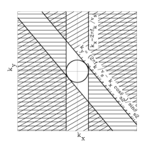
Figure 1: Graphical representation of the three classes of modes enumerated in section II.2. Left Panel: Phasor plot of modes for a single $k=|\bm{k}|$. For two observations at scan angles $\theta_{\mathrm{s}1}$ and  $\theta_{\mathrm{s}2}$, modes which fall within $\theta_{\mathrm{c}}$ of either $\theta_{\mathrm{s}1}$ or $\theta_{\mathrm{s}2}$ but not both – indicated by the singly hatched regions – will have variance $\sigma^{2}_{\mathrm{w}}/N_{\mathrm{s}}$; modes which fall within $\theta_{\mathrm{c}}$ of both $\theta_{\mathrm{s}1}$ and $\theta_{\mathrm{s}2}$ – indicated by the doubly hatched region – will have variance $\sigma^{2}_{\mathrm{w}}/2N_{\mathrm{s}}$; modes which lie further than $\theta_{\mathrm{c}}$ from both $\theta_{\mathrm{s}1}$ and $\theta_{\mathrm{s}2}$ (non-hatched regions) will have infinite variance. Right Panel: 2-d Fourier-space representation of these classes of modes at all $k$ for $\theta_{\mathrm{s}1}=0^{\circ}$ and $\theta_{\mathrm{s}2}=40^{\circ}$. The circle at the center has radius $2\pi f_{\mathrm{knee}}/v_{\mathrm{s}}$ and indicates the modes that will have infinite variance no matter how many different scan angles are used.

To get the minimum-variance estimate of the CMB power spectrum from these three classes of modes, we estimate $P(k)$ using each class individually and make a weighted mean of these estimates using inverse-variance weighting based on equation 15. In the noise-dominated regime (where $\sigma^{2}_{\mathrm{w}}/N_{\mathrm{s}}\gg P(k)$), the variance on our measurement of the CMB power spectrum from these combined observations will be:

$$\big{[}\delta P(k)\big{]}^{2} = \frac{1}{\sum_{|\bm{k}_{i}|=k}\big{[}\delta P(\bm{k}_{i})\big{]}^{-2}}$$

$$= \left[\frac{N_{2}(k)}{(\sigma^{2}_{\mathrm{w}}/N_{\mathrm{s}})^{2}}+\frac{N_{1}(k)}{(\sigma^{2}_{\mathrm{w}}/2N_{\mathrm{s}})^{2}}\right]^{-1}$$

$$= \big{[}\delta P_{\mathrm{no}1/f}(k)\big{]}^{2}\left[\frac{N_{2}(k)}{4N_{\mathrm{tot}}(k)}+\;\frac{N_{1}(k)}{N_{\mathrm{tot}}(k)}\right]^{-1},$$

where we have identified the prefactor in equation II.2

$$\big{[}\delta P_{\mathrm{no}1/f}(k)\big{]}^{2} = \frac{2}{N_{\mathrm{tot}}(k)}\left[P(k)+\frac{\sigma^{2}_{\mathrm{w}}}{2N_{\mathrm{s}}}\right]^{2}$$

$$= \frac{\sigma^{4}_{\mathrm{w}}}{4N_{\mathrm{s}}^{2}\;kf_{\mathrm{sky}}\Delta k}\;\mathrm{if}\;\sigma^{2}_{\mathrm{w}}/N_{\mathrm{s}}\gg P(k)$$

as the variance our combined measurements would have if the instrument noise were equal to the high-frequency white-noise value at all temporal frequencies (i.e., without the $1/f$ noise component). The ratio of variance in the presence of our toy-model $1/f$ noise to the variance with no $1/f$ noise (still assuming $\sigma^{2}_{\mathrm{w}}/N_{\mathrm{s}}\gg P(k)$) evaluates to

$$\left[\frac{\delta P(k)}{\delta P_{\mathrm{no}1/f}(k)}\right]^{2}=\frac{\pi}{\theta_{\mathrm{c}}}$$ (28)

in the independent-modes case (where $\left|\theta_{\mathrm{s}1}-\theta_{\mathrm{s}2}\right|>2\theta_{\mathrm{c}}(k)$) and to

$$\left[\frac{\delta P(k)}{\delta P_{\mathrm{no}1/f}(k)}\right]^{2}=\frac{\pi}{2\theta_{\mathrm{c}}-\left|\theta_{\mathrm{s}2}-\theta_{\mathrm{s}1}\right|/2}$$ (29)

in the overlapping-modes case (where $\left|\theta_{\mathrm{s}1}-\theta_{\mathrm{s}2}\right|\leq 2\theta_{\mathrm{c}}(k)$).

Equations 28 and 29 contain the potentially surprising result that in the noise-dominated regime, the best constraints on $P(k)$ are obtained by reobserving the sky at the same scan angle (so that $|\theta_{\mathrm{s}2}-\theta_{\mathrm{s}1}|=0$). That is to say, the scan strategy without cross-linking outperforms the cross-linked strategy. It is trivial to show that in the sample-variance-dominated regime (where $P(k)\gg\sigma^{2}_{\mathrm{w}}/N_{\mathrm{s}}$), one comes to the opposite conclusion, namely that the best constraints are obtained in the minimally cross-linked strategy. In fact, the question being considered here is very similar to that of optimizing sky coverage vs. observing time per pixel in a CMB experiment. In our case the question is how to divide observing time between Fourier modes rather than spatial pixels, but the optimization calculation is the same.

II.3 Results for “real” $1/f$ noise

The approximation in equation 13 leads to a concise, illustrative result, but there is no reason we cannot do the calculation for noise with a true $1/f$ spectrum (as defined in equation 12). For a single observation at scan angle $\theta_{\mathrm{s}}$, our best inverse-variance weighted estimate of $P(k)$ will have variance:

$$\big{[}\delta P(k)\big{]}^{2} = \frac{\pi}{2kf_{\mathrm{sky}}\Delta k}\times$$

$$\Bigg{\{}\int_{0}^{\pi/2}d(\theta_{k}-\theta_{\mathrm{s}})\Bigg{[}P(k)+$$

$$\frac{\sigma^{2}_{\mathrm{w}}}{N_{\mathrm{s}}}\left(1+\frac{2\pi f_{\mathrm{knee}}}{kv_{\mathrm{s}}\cos(\theta_{k}-\theta_{\mathrm{s}})}\right)\Bigg{]}^{-2}\Bigg{\}}^{-1}.$$

Optimally combining two observations at $\theta_{\mathrm{s}1}$ and $\theta_{\mathrm{s}2}$ yields a power spectrum measurement with variance:

$$\big{[}\delta P(k)\big{]}^{2} = \frac{2\pi}{kf_{\mathrm{sky}}\Delta k}\Bigg{\{}\int_{0}^{2\pi}d\theta_{k}$$

$$\left[P(k)+\frac{\sigma^{2}_{\mathrm{w}}}{N_{\mathrm{s}}}(1+q_{1})||(1+q_{2})\right]^{-2}\Bigg{\}}^{-1},$$

where

$$q_{i}=\frac{2\pi f_{\mathrm{knee}}}{kv_{\mathrm{s}}\left|\cos(\theta_{k}-\theta_{s,i})\right|},$$ (32)

and the parallel operator is defined such that

$$x_{1}||x_{2}=\left[\frac{1}{x_{1}}+\frac{1}{x_{2}}\right]^{-1}.$$ (33)

Once again, the relative performance of the non-cross-linked and minimally cross-linked strategies depends on the relative size of the noise and sample variance. Figure 2 shows the ratio of $\delta P(k)$ to the value we would obtain with no $1/f$ noise for the two scan strategies and two noise- vs. sample-variance regimes under consideration, using realistic values of $v_{\mathrm{s}}$ and $f_{\mathrm{knee}}$.

Figure 2: Ratio of $\delta P(k)$ to the no-$1/f$-noise value for the non-cross-linked (solid line) and minimally cross-linked (dashed line) scan strategies in two regimes of noise variance vs. sample variance. Upper curves: $P(k)=\sigma^{2}_{\mathrm{w}}/N_{\mathrm{s}}/40$. Lower curves: $P(k)=40\ \sigma^{2}_{\mathrm{w}}/N_{\mathrm{s}}$. In both cases, the observational parameters are: $f_{\mathrm{knee}}=0.1\mathrm{Hz}$ and $v_{\mathrm{s}}=1^{\circ}/\mathrm{s}$. In the minimally cross-linked cases, $\theta_{\mathrm{s}2}=\theta_{\mathrm{s}1}+90^{\circ}$.

Though the difference in the two strategies is less dramatic than the factor of $\sqrt{2}$ in the toy model case (see equations 28 and 29), the behavior is qualitatively similar. In the noise-variance-dominated regime, the power spectrum sensitivity is dominated by the best-measured modes, in which case it is advantageous to concentrate observing time on measuring a small number of modes very well; in the sample-variance-dominated regime, sensitivity is equal among all modes that are measured well enough to get below the sample variance, in which case it is better to spread the observing time around and measure as many modes as possible just well enough.

II.4 Results for other choices of scan parameters

While the most important conclusion to be drawn from figure 2 is the relative performance between the non-cross-linked and minimally cross-linked strategies, the amplitude of $\delta P(k)$ for both strategies compared to the case with no $1/f$ noise is also of interest. Not surprisingly, in the noise-variance-dominated regime, the value of $k$ at which the $1/f$ noise begins to dominate $\delta P(k)$ is very close to what would naively expect, namely

$$k(1/f)=\frac{2\pi f_{\mathrm{knee}}}{v_{\mathrm{s}}}.$$ (34)

For the particular values of $f_{\mathrm{knee}}$ and $v_{\mathrm{s}}$ used in figure 2 ($f_{\mathrm{knee}}=0.1\mathrm{Hz}$ and $v_{\mathrm{s}}=1^{\circ}/\mathrm{s}$), which are realistic approximations for the upcoming generation of CMB experiments, $k(1/f)=36$, indicating that for an experiment which meets these criteria, $1/f$ noise will not limit observations at least down to the $\ell\sim 100$ range (recall that we are working in the flat-sky regime where $\ell\sim k$). As for experiments which have different values of $f_{\mathrm{knee}}$ and $v_{\mathrm{s}}$, a quick glance at equations II.3 - 33 makes it clear that for the noise-variance-dominated case, the results in figure 2 can be scaled from the values for $f_{\mathrm{knee}}$ and $v_{\mathrm{s}}$ used in the plot to arbitrary values by scaling the x-axis using equation 34.

The other key observing strategy design parameter for raster-scanned experiments is the size and geometry of the sky patch observed in one full raster. The results in figure 2 are unaffected by changes in sky patch size and geometry (which only come into equation II.3 in the $f_{\mathrm{sky}}$ term, which itself drops out when we normalize to the no-$1/f$ case), except in that the extent of the largest dimension of the patch puts a fundamental lower limit on the $k$- (or $\ell$-) modes that can be measured.

III Discussion

III.1 Comparison with earlier work

The results of equations 28 and 29 and figure 2 seem in direct contradiction to the conventional wisdom that cross-linking — however minimal — is vital to CMB power spectrum sensitivity in the presence of $1/f$ noise. In particular, (Tegmark, 1997, T97) found an order-of-magnitude difference in $P^{\mathrm{noise}}(k)$ for two scan strategies very much like our non-cross-linked and minimally cross-linked ones (cf. T97’s “Serpentine” and “Fence” scans). However, the quantity plotted in T97 is effectively the noise power averaged over all modes of a given $k$ (cf. T97, equation 52), whereas the total instrument sensitivity to signal at a given $k$ is proportional to the sum of the weight, or the inverse noise power, over all modes of that $k$. The key to reconciling our result and that of T97 is to understand that the excess noise power in the non-cross-linked or Serpentine scan is concentrated in a few easily identifiable bad modes, and that the remaining good modes are actually measured better in this scan strategy than in the minimally cross-linked, or Fence scan. When the inverse noise power is summed over all modes of a given $k$, it is the repeated measurement of the good modes that wins out over measuring new modes — at least in the noise-variance-dominated regime.

IV Conclusion

We have calculated the sensitivity to the CMB power spectrum (or any other angular power spectrum) for a raster-scanned instrument in the presence of $1/f$ noise and compared this sensitivity in the non-cross-linked and minimally cross-linked cases. We have shown that in the noise-variance-dominated regime, the non-cross-linked scan strategy actually outperforms the minimally cross-linked scan strategy. From the viewpoint of noise sensitivity alone (i.e., not taking into account systematic contaminants such as ground pickup or chopping mirror offsets), this result indicates that CMB instruments that are unable to easily cross-link scans are at no disadvantage.