Weak Lensing of Baryon Acoustic Oscillations

Abstract

Baryon Acoustic Oscillations (BAO) have recently been observed in the distribution of distant galaxies. The height and location of the BAO peak are strong discriminators of cosmological parameters. Here we consider the ways in which weak gravitational lensing distorts the BAO signal. We find two effects that can affect the height of the BAO peak in the correlation function at the percent level but that do not significantly impact the position of the peak and the measurement of the sound horizon. BAO turn out to be robust cosmological standard rulers.

I Introduction

In the early universe, before the recombination of protons and electrons into neutral hydrogen, the photons, electrons, and protons were tightly coupled and behaved like a single fluid. The density of this fluid underwent acoustic oscillations until recombination. These oscillations left their imprints in the spectrum of anisotropies in the cosmic microwave background (CMB) as well as in the distribution of matter via the correlation function of the galaxy distribution. The effect in the former case is quite pronounced because the photons have essentially traveled freely since their last scattering at recombination. In the latter case, called baryon acoustic oscillations (BAO), the effect is diluted since the dominant dark matter did not participate in the primordial dance Meiksin et al. (1998); Seo and Eisenstein (2003); Blake and Glazebrook (2003); Hu and Haiman (2003). Observations of both of these effects over the last few years Spergel et al. (2006); Eisenstein et al. (2005) provide dramatic proof that our picture of the early universe is consistent.

We are now free to go further and use these observations to constrain cosmological parameters. In the case of BAO, the correlation function should peak at a comoving scale of order $r_{p}\simeq 100h^{-1}$Mpc where the Hubble constant is parameterized as $H_{0}=100h$ km sec^-1 Mpc^-1. In a survey of galaxies at the same redshift, the peak shows up at an angular scale $\delta\theta=r_{p}/[(1+z)D_{A}(z)]$ where $D_{A}(z)$ is the angular diameter distance out to redshift $z$. In a 1D radial survey with redshifts, the peak will show up at $\delta z=r_{p}H(z)$. More generally, in a 3D survey, one can hope to measure both $D_{A}(z)$ and $H(z)$. These quantities are enormously important to cosmologists because they depend on the energy density back to redshift $z$ and therefore on the properties of matter and dark energy Copeland et al. (2006); Uzan (2006); Peacock et al. (2006); Albrecht et al. (2006). Besides its location, the height of the BAO peak is governed by the matter density $\Omega_{m}h^{2}$ Eisenstein and Hu (1998).

For these reasons, a number of ambitious future surveys have been proposed aiming to measure the BAO peak at multiple redshifts with very high accuracy Bassett et al. (2005); Peacock et al. (2006). Roughly, one expects to measure $D_{A}$ from the acoustic scale with an accuracy Peacock et al. (2006) $(V/5h^{-3}\,{\rm Gpc})^{-1/2}(k_{\rm max}/0.2h\,{\rm Mpc}^{-1})^{-1/2}$ where $V$ is the volume of the survey, and $k_{\rm max}$ is the comoving wavenumber at which the power spectrum peaks. Currently for the Sloan Digital Sky Survey (SDSS), the error is of order $4\%$ at $z\sim 0.4$ Eisenstein et al. (2005). These errors are expected to go down Aubourg (2007) to  $2.8\%$ at $z\sim 0.4$ by 2008 when SDSS has accumulated 8000 square degrees; to $1.1\%$ at $z\sim 0.6$ and $1.4\%$ at $z\sim 2.5$ (SDSS-III, 10000 deg²); $1\%$ at $z\sim 1$ and $1.5\%$ at $z\sim 2.8$ (SUBARU+NOAO, 2013); and $1.2\%$ at $z\sim 0.4,0.6,1$ (GWFMOS, 2000 deg²). Amid this excitement, many studies have been carried out searching for sources of systematic errors in BAO measurement Guzik and Bernstein (2006); Huff et al. (2007); Eisenstein et al. (2006) focusing mostly on the non-linear evolution of structure, scale-dependent bias and errors in the survey window function estimation, the first two leading to effects smaller than a percent on $D_{A}$ while the latter has to be kept below 2% not to bias the acoustic scale by more than 1% at $z=1$. Given the great wealth of data that will become available, the present analysis focuses mainly on galaxy surveys and on the resulting galaxy correlation function. It is necessary to stress, however, that the same kind of analysis can be applied equally well to the two point correlation function of different classes of objects, notably the $10^{5}$ high redshift QSO that are expected to be surveyed by SDSS-III.

In this paper we show that weak lensing is not necessarily negligible at the level of accuracy that will be attained by future surveys. This effect is reminiscent of the weak lensing of Type Ia supernovae that induces an external dispersion in their observed brightnesses, comparable in magnitude to the intrinsic dispersion for redshifts $z>1$ Dalal et al. (2003); Williams and Song (2004); Wang (2005); Menard and Dalal (2005). In that case, the main effect of lensing is to magnify the background objects; in this case, while magnification can cause one effect, distortion of the BAO rings leads to an additional effect.

Light is deflected by large scale structure as it travels from sources in a deep survey to us, and this lensing leads to two sources of error in BAO. First, the position we assign to a given galaxy based on its redshift and angular position on the sky does not correspond to its actual position. When we measure the correlation function by assigning distance to all pairs of galaxies, we are therefore inevitably making an error. We place a pair of galaxies in a given distance bin, but they may well belong in a different bin. This effect tends to smooth out features in the correlation function so will not change the position of the BAO peak but will change its height and width. An almost identical effect acting on the CMB is well-known (see Ref. Lewis and Challinor (2006) for a recent review) and now even included in the codes which compute the CMB spectrum.

In the case of a galaxy (or QSO) survey, there is a second effect that does not affect the CMB. Surveys are generally magnitude limited, so they include only objects brighter than some threshold. Not only does lensing change the apparent position of galaxies, but it also changes their magnitude Mellier (1999); Bartelmann and Schneider (2001): it will brighten some galaxies, otherwise too faint to be detected, and push them over threshold and de-magnify others, causing them to drop out of the survey. This effect, dubbed magnification bias, is also well-known especially in studies of the correlation between quasars and galaxies Ménard and Bartelmann (2002); Matsubara (2000) where it has been detected Scranton et al. (2005); Myers et al. (2005); Mountrichas and Shanks (2007). Its effect induces a non-zero contribution to the correlation function even if the underlying galaxy population was completely random Moessner and Jain (1997); Jain (2002).

The paper is organized as follows. In Sec. II we explicitly compute the effect of the re-mapping due to the lensing and the smoothing it induces on the correlation function. In Sec. III we then turn to the analysis of the magnification bias. In Sec. IV we discuss the impact of these two effects on BAO measurements. Finally, all the technicalities are gathered in the Appendices.

II Smoothing of the Correlation Function

The effect we consider in this section arises because photons travel on geodesics and these in turn depend on the energy density distribution present between the source and the observer. This implies that the observed position of a source galaxy (denoted by $\vec{x}_{o}$) and its actual position (denoted by $\vec{x}_{s}$) will in general differ. The galaxy number overdensity at a given position $\vec{x}$ is defined by

$$\delta^{g}(\vec{x})\equiv\frac{n(\vec{x})-\bar{n}}{\bar{n}},$$ (1)

where $n(\vec{x})$ is the galaxy number density at position $\vec{x}$ and $\bar{n}$ is the mean density that would be measured if all galaxies were uniformly distributed.

The correlation function is defined as the two point function of the observed $\delta$ field. The observed, lensed correlation function will in general differ from the unlensed correlation function. What is actually measured is the correlation between galaxies overdensities at observed positions

$$\xi_{\rm{obs}}(r)=\xi_{GG}(r)\equiv\langle\tilde{\delta}^{g}(\vec{x}_{o})\tilde{\delta}^{g}(\vec{x}^{\prime}_{o})\rangle_{|\vec{x}_{o}-\vec{x}^{\prime}_{o}|=r},$$ (2)

The unlensed correlation function on the other hand is the correlation between overdensities at actual source positions $\xi_{s}(r)$. Since we are interested in large scales, in what follows we assume a linear bias model (not depending on scales or redshift Simon et al. (2006)) so that galaxies trace the underlying dark matter fluctuations and $\delta^{g}(\vec{x})=b\delta(\vec{x})$. This assumption in turn implies that galaxies and matter overdensity correlation functions (resp. denoted by $\xi_{GG}$ and $\xi$) are simply related by a multiplicative constant $b^{2}$: in what follows we focus on the latter even though the results apply to the former as well. To find the connection between the lensed and unlensed correlation functions, we use the fact that weak lensing induces a re-mapping of the density field as $\tilde{\delta}(\vec{x}_{o})=\delta(\vec{x}_{s})$ where the two positions are related by the displacement vector field as $\vec{x}_{o}=\vec{x}_{s}+\vec{\zeta}(\vec{x}_{s})$. A Taylor expansion leads

$$\tilde{\delta}(\vec{x}_{o})=\delta(\vec{x}_{s})+\frac{\partial\delta}{\partial x_{i}}\zeta^{i}+\frac{1}{2}\frac{\partial^{2}\delta}{\partial x^{i}\partial x^{j}}\zeta^{i}\zeta^{j},$$ (3)

where we have kept terms up to second order in the displacement. It follows that (see Appendix A for details)

$$\xi_{\rm{obs}}(r) = \xi_{s}(r)+\delta\xi_{sm}(r),$$ (4)

$$\delta\xi_{sm}(r) = \left[\langle\zeta^{i}(\vec{x})\zeta^{j}(\vec{x})\rangle-\langle\zeta^{i}(\vec{x})\zeta^{j}(\vec{y})\rangle\right]$$ (5)

$$\times \left[\frac{\delta^{ij}}{r}\frac{{\rm d}\xi(r)}{{\rm d}r}+\frac{r^{i}r^{j}}{r}\frac{{\rm d}}{{\rm d}r}\left(\frac{\xi^{\prime}(r)}{r}\right)\right].$$

In this expression the effect of lensing appears only at second order because $\langle\vec{\zeta}\rangle=0$.

The additional term $\delta\xi_{sm}$ is due to lensing and tends to smooth out the correlation function. A simple way to understand it is to think of the BAO peak as a circle on the sky. When the light from this circular feature passes through an overdense line-of-sight, it will appear larger so the feature will move to larger radius. Conversely, it can appear smaller if the intervening matter is underdense. Since there is an excess of circles at the peak scale, most fluctuations will push a circle out of the peak bin and into an adjacent bin. The net result is that the peak will be smoothed out: the correlation function will be enhanced below and above the peak and reduced at the peak. This is encoded in equation (5). To further understand this effect, let us consider the two factors appearing in the lensing term separately. The zero-lag two-point function $\langle\zeta^{i}(\vec{x})\zeta^{j}(\vec{x})\rangle$ is simply the variance of the deflection distance while $\langle\zeta^{i}(\vec{x})\zeta^{j}(\vec{y})\rangle$ is the correlation between the deflection experienced by two light rays emitted a distance $r$ from one another. If $r$ is very small, then $\langle\zeta^{i}(\vec{x})\zeta^{j}(\vec{y})\rangle$ will be very close to $\langle\zeta^{i}(\vec{x})\zeta^{j}(\vec{x})\rangle$, that is, two galaxies separated by $r$ will have their geodesics deflected by the same amount. In that case, the terms in the first set of square brackets will cancel and there will be no effect: the circles on the sky will simply be shifted with no distortion in their sizes. However, if $r$ is large enough then there will be little correlation between the deflections of galaxies separated by $r$ and the second term will be smaller than the first. Moving on to the second set of square brackets, notice that the smoothing term can be significant where the first or the second derivative are large. This in turn implies that the departure of $\xi_{o}(r)$ from $\xi_{s}(r)$ can become non-negligible especially in the region of the BAO peak.

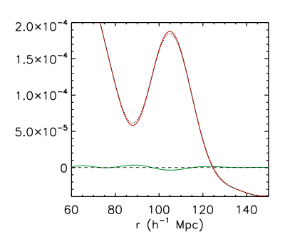
Figure 1: Correction due to position re-mapping for background galaxies at $z=2.5$. Solid red curve is the galaxy-galaxy correlation function assuming a constant bias factor $b=1$. Green solid is the re-mapping term. Around $r=100h^{-1}$Mpc it is negative while on either side it is positive. In other words lensing smooths out the BAO peak, as can be seen directly from the dotted curve which includes both contribution.

As shown in Appendix B, adopting the Limber approximation all the terms appearing in equation (5) can be recast as integrals over the dark matter power spectrum. The smoothing correction can then be expressed as

$$\delta\xi_{sm}(r)=\xi^{\prime\prime}\left(\frac{I_{1}}{2}-I_{2}+I_{3}\right)+\frac{\xi^{\prime}}{r}\left(\frac{I_{1}}{2}-I_{3}\right),$$ (6)

where

$$I_{i}\equiv\frac{9\Omega_{m}^{2}H_{0}^{4}}{4}\int\!\!\frac{{\rm d}k}{2\pi k}\int_{0}^{\chi_{s}}{\rm d}\chi\,W^{2}(\chi_{s},\chi)P_{\delta}(k,\chi)K_{i}(k,\chi),$$ (7)

$$K_{i}(k,\chi)\equiv\left\{\begin{array}[]{ll}1,&i=1\\ J_{0}(k\chi),&i=2\\ J_{1}(k\chi)/(k\chi),&i=3\end{array}\right.$$ (11)

and where $W(\chi_{s},\chi)=2\chi_{s}(1-\chi/\chi_{s})$ is the window function, $\chi_{s}$ is the comoving distance to the source, and a flat FRW background is assumed throughout. We integrate over the fully evolving nonlinear power spectrum using the procedure of Smith et al. Smith et al. (2003). The results are depicted in Fig. 1, for simplicity in the case where all galaxies are at the same redshift. We see that smoothing occurs at the percent level, not a surprising result given similar conclusions in the case of the CMB. Nonetheless, this smoothing may need to be accounted for when analyzing future surveys. This fact is further stressed in Fig. 2, where the ratio between the smoothing term and the full correlation function is plotted for the redshift range that likely will be probed by future surveys.

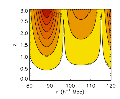
Figure 2: Absolute value of the ratio of the correlations due to position re-mapping and the galaxy-galaxy correlation function. The lensing contribution is of the order of a few percent in the region where the correlation function exhibits the BAO peak.

There are some important conclusions to be drawn from this analysis. First, this lensing-induced correlation is unavoidable and has nothing to do with the way measurements are carried out. This means that such a contribution will arise even if the “perfect survey” with an infinite limiting magnitude is carried out, simply because geodesics are sensitive to the matter distribution present between the source and the observer. Second, the previous derivation does not depend in any way on the class of objects that are being surveyed: it can be applied equally well to future QSO catalogs. Third, although the corrections to the correlation function are larger than a percent, these corrections do not alter the BAO peak position. For example, at $z=2.5$ this lensing-induced correlation weights about $1.5\%$, but the shift in the peak position is only $0.01\%$. BAO therefore turn out to be standard rulers that are very robust with respect to this effect. Finally, the dominant contributions to the lensing-induced terms arise from modes that are still in the linear regime: we carried out the integrations using the fully evolving nonlinear power spectrum, but the results do not change if the linear power spectrum is used. Physically this is because it is large structures that are most responsible for deflections; the $k$-integral in equation (7) peaks at the same place the power spectrum does, roughly $k\simeq 0.02h$Mpc^-1, deep in the linear regime. An important implication of this is that the correction is very easy to implement.

III Magnification Bias

We now move to consider a second, different effect that can also impact the determination of the correlation function and the measurement of the BAO peak position. While the effect analyzed in the previous section was an unavoidable consequence of any metric theory of gravity and of the rich structure in the universe, the effect considered here is related to the fact that actual surveys include only objects that are brighter than a limiting threshold.

Weak gravitational lensing acts in two ways when such surveys are carried out. First, it can brighten some objects pushing them over the threshold and de-magnify others causing them to drop out of the survey. Second, it can stretch a given patch of sky making it larger or smaller than it actually is, thus increasing or decreasing the measured number density. If $n_{0}(f,z)$ is the number of objects with flux larger than $f$ per unit solid angle between $z$ and $z+{\rm d}z$ in the absence of lensing, the observed number density in direction $\hat{n}$ will be $n_{0}[f/\mu(\hat{n},z),z]/\mu(\hat{n},z)$ where $\mu[(\hat{n},z),z]=1/[(1-\kappa)^{2}-\gamma^{2}]$ is the magnification expressed in terms of the convergence $\kappa$ and the shear amplitude $\gamma$. In the simple case where $\mu$ is assumed independent of $z$, this implies that $n(m,\hat{n})=n_{0}(m)[\mu(\hat{n})]^{2.5s-1}$ where $s$ is the slope of the number density as a function of the magnitude $m$, $s\equiv{\rm d}\ln n_{0}(m)/{\rm d}m$. Focusing for the time being on the correlation function for galaxies, it is important to keep in mind that the magnitude and the sign of this effect (over- or under-density for $\mu>1$) depends on the slope of the luminosity function, which in turn is different for different classes of objects and can present redshift evolution Scarlata et al. (2006).

Proceeding along the same lines of the analysis carried out by Moessner and Jain Moessner and Jain (1997) on the angular correlation function, we find that the fluctuation in the galaxy number density at a given position $\delta(\vec{x})$ receives contributions from two sources: the true galaxy clustering, denoted by $\delta^{g}(\vec{x})$ and the variation in the number density due to magnification of the galaxy population induced by lensing, denoted by $\delta^{l}(\vec{x})$. The observed overdensity is the sum of these two, $\delta(\vec{x})\equiv\delta^{g}(\vec{x})+\delta^{l}(\vec{x})$, so

$$\xi_{\rm{obs}}(r) = \langle\delta(\vec{x})\delta(\vec{y})\rangle=\langle\delta^{g}(\vec{x})\delta^{g}(\vec{y})\rangle+\langle\delta^{g}(\vec{x})\delta^{l}(\vec{y})\rangle$$ (12)

$$+ \langle\delta^{l}(\vec{x})\delta^{g}(\vec{y})\rangle+\langle\delta^{l}(\vec{x})\delta^{l}(\vec{y})\rangle.$$

where $|\vec{x}-\vec{y}|=r$.

The first term in Eq. (12) is the true galaxy-galaxy correlation function. As mentioned in the previous section, in the linear bias approximation this term is directly proportional to the matter correlation function.

$$\langle\delta^{g}(\vec{x})\delta^{g}(\vec{y})\rangle=\xi_{GG}(r)=b^{2}\xi(r).$$ (13)

The second and third terms are the contributions to the observed correlation function arising from correlating a galaxy overdensity arising because of lensing along the line of sight with a true matter overdensity. The last term is the contribution to the correlation function due to two overdensities which are generated both because of lensing along the line of sight to the source galaxies.

We now consider the two cross terms $\langle\delta^{g}(\vec{x})\delta^{l}(\vec{y})\rangle$. These arise from the correlation of overdensities due to clustering with an apparent overdensity due to lensing. To proceed further, let us recall the expression for $\delta^{l}$ originally derived by Broadhurst, Taylor and Peacock Broadhurst et al. (1995) and also used in Moessner and Jain Moessner and Jain (1997)

$$\delta^{l}(\vec{x})=(5s-2)\kappa(\vec{x}),$$ (14)

where as before $s$ is the logarithmic slope of the number counts. The convergence is determined by an integral along the line of sight

$$\kappa(\vec{y})\equiv\frac{3\Omega_{m}H_{0}^{2}}{2}\int_{0}^{\chi_{s}(\vec{y})}{\rm d}\chi W_{L}(\chi_{s},\chi)\frac{\delta(\vec{y},\chi)}{a},$$ (15)

where $\chi_{s}$ is the comoving distance to the source galaxy and $W_{L}(\chi_{s},\chi)\equiv\chi(\chi_{s}-\chi)/\chi_{s}$ is the lensing geometric factor. Using this relation, we derive (see Appendix C) that

$$\xi_{GL}(r)\equiv\langle\delta^{g}\delta^{l}\rangle=Cbr\frac{1+\chi_{s}a(\chi_{s})H(\chi_{s})}{a(\chi_{s})\chi_{s}}I_{gl},$$ (16)

where for sake of brevity we have defined the constant

$$C\equiv\frac{3}{2}(5s-2)\Omega_{m}H_{0}^{2},$$ (17)

and the integral

$$I_{gl}\equiv\int\frac{{\rm d}k}{2\pi}P_{\delta}(k,z)J_{1}(kr),$$ (18)

where $J_{1}(x)$ is the Bessel function of the first kind. The factor of $r$ in the prefactor of Eq. (16) indicates that not all lensing matter along the line of sight contributes to this cross term. Rather, only within a distance $r$ are regions with more galaxies likely to produce a larger lensing signal. If there is a huge excess of matter along the line of sight but far from the source galaxy, the magnification it produces will just as likely be associated with a background underdensity as overdensity, so the correlation $\langle\delta^{g}\delta^{l}\rangle$ due to it will be zero. As a result, this cross term will be largest for low redshift background galaxies. After all, the matter field is more clustered at late times, and the cross term is most sensitive to clustering at the background galaxy redshift. Fig. 3 verifies these two features. The cross term is indeed very small and does get smaller as one moves to higher redshift.

We now turn to the lensing-lensing term in the correlation function, which is explicitly given by (see Appendix C)

$$\xi_{LL}(r)\equiv\langle\delta^{l}\delta^{l}\rangle=C^{2}\int_{0}^{\chi_{s}}{\rm d}\chi\left[\frac{W_{L}(\chi_{s},\chi)}{a(\chi)}\right]^{2}I_{ll}(\chi),$$ (19)

where in this case

$$I_{ll}(\chi)\equiv\int\frac{k\,{\rm d}k}{2\pi}J_{0}(kr)P_{\delta}(k,\chi).$$ (20)

Here there is no prefactor of $r$: all structures along the line of sight can contribute. As a result, this term is largest when the background galaxies are at high redshifts and can get lensed by as much structure as possible.

The result of the calculation of these three contributions is shown in Fig. 3, where $(2.5s-1)=1$ is assumed and the integrations are carried out considering the fully evolving non-linear power spectrum obtained applying the procedure of Smith et al. Smith et al. (2003). Four sets of curves are obtained, corresponding to sources at redshift of 0.5, 1, 2, 3. From Fig. 3, we see that while the amplitude of $\xi_{GG}$ and $\xi_{GL}$ decreases for increasing redshift, the amplitude of $\xi_{LL}$ increases for increasing redshift, thus contributing more and more to the full correlation function.

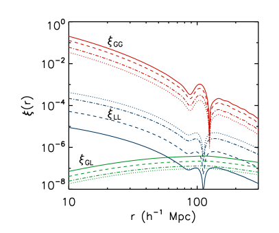
Figure 3: Correlation functions at different redshifts: $\xi_{GG}$ (red), $\xi_{GL}$ (green) and $\xi_{LL}$ (blue). In each case solid curves corresponds to galaxies at $z=0.5$, dashed curves $z=1$, dot-dashed curves $z=2$ and dotted curves $z=3$. For illustration purposes here we set $b=1$ and $2.5s-1=1$ and we assume a flat FRW universe with $\Omega_{m}=0.3$ and $\Omega_{\Lambda}=0.7$.

In Fig. 4 two sets of curves are shown, obtained integrating either over the non-linear power spectrum of Smith et al. Smith et al. (2003) or over the linear power spectrum. We see that non-linearities significantly contribute to the correlation function on scales that are much smaller than the ones where the BAO peak is located. As in the case of the lensing-induced correlations considered in the previous section, this result implies that our conclusions do not depend on the details of the non-linear evolution of structure.

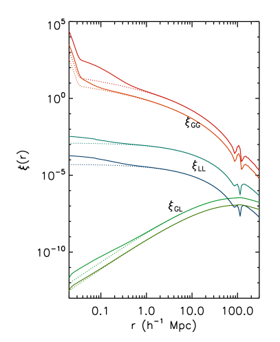
Figure 4: Calculations of the $\xi_{GG}$, $\xi_{GL}$ and $\xi_{LL}$ terms carried out for $z=0.5$ (darker curves) and $z=2.0$ (lighter curves). The solid lines are obtained integrating over the fully evolving non-linear power spectrum obtained using the procedure of Smith et al. Smith et al. (2003), while the dotted ones are obtained integrating over the linear power spectrum. In the range where the correlation function exhibits the BAO peak non-linearities do not significantly contribute. Again, $b=1$ and $2.5s-1=1$ are assumed for illustration purposes.

It is now necessary to stress that equations (16) and (19) respectively depend linearly and quadratically on the factor $(2.5s-1)$. This factor is crucial in determining the weight of the magnification bias contribution to the correlation function of the class of objects considered. In particular, despite the fact that the actual values of $s$ depend on the survey, they are smaller for galaxies ($s\sim[0.2,0.6]$) Fort et al. (1996); Yasuda et al. (2001) than for QSO ($s\sim[-2,1.6]$) Scranton et al. (2005); Menard and Peroux (2003). This means that the $(2.5s-1)$ factors appearing in front of the magnification bias terms are smaller (larger) than unity for galaxies (QSO): while the magnification bias is suppressed for the galaxy correlation function, it can actually play a significant role for the QSO correlation function. This in turn strengthens the conclusion of the previous section and points toward a well defined class of objects: BAO measured through the correlation function of galaxies represent very robust standard rulers, only marginally affected by lensing even at moderately high redshifts. By the same token, given the scaling of the magnification bias terms with respect to $C$, the correlation function of QSO da Angela et al. (2006) can receive significant contributions from the lensing-lensing term, especially at high redshift. If one is interested in extracting information from the lensing-lensing signal, then the QSO correlation function seems the way to go.

IV Discussion

To understand the role of lensing, recall that the measurement of the BAO bump appearing in the correlation function conveys information about two physical scales Eisenstein and Hu (1998); Hu and Dodelson (2002). The centroid of the bump is related to the sound horizon, that is the comoving distance that a sound wave can travel between the big bang and recombination. The amplitude of the bump on the other hand is directly related to the matter-radiation equality period. We have shown that weak lensing can affect the measurement of baryon acoustic oscillation through the correlation function in two very different ways.

First, weak lensing smooths out the acoustic peak in the correlation function. This smoothing is unavoidable, even if the “perfect survey” could eventually be carried out. This lensing-induced term smooths the BAO peak at the level of a few percent but the peak location does not change because of it. In other words lensing does not affect the measurement of the sound horizon. On the other hand, the measurement of the matter-radiation equality period (and thus of $\Omega_{m}h^{2}$ Eisenstein et al. (2005)) depends on the peak amplitude and it can therefore be affected at the percent level.

Second, weak lensing can also contribute a magnification bias term to the correlation function that adds to the unlensed term and that can potentially obscure the prominent feature of interest. This magnification bias contributes in different ways depending on the class of objects used to measure the correlation function. In particular, while it can significantly affect the correlation function of QSO, magnification bias turns out to be only marginal for galaxy surveys.

After taking both effects into account, we conclude that the BAO feature in the galaxy correlation function is a robust standard ruler. For instance, in the case in which all surveyed galaxies are at $z=2.5$, the lensing-induced correlation is of order $1.5\%$, but the location of the BAO peak shifts by only $0.01\%$. The same cannot be said about possible QSO correlation function, however, since in that case magnification bias (notably, the lensing-lensing term) can play a significant role.

Finally, let us remark that the sensitivity of the results reported in Sec. II and III on the linear bias parameter $b$ is different for the different effects. While both the lensing induced smoothing and the magnification bias would be affected by a scale dependence of the bias factor, the former would not be sensitive to a change in the overall magnitude of $b$. On the other hand, if in the future evidence of “antibias” will surface (as suggested by the recent work of Simon et al. Simon et al. (2006)) this will lead to an enhancement of the magnification bias. Since $\xi_{GG}$ depends quadratically on $b$ while $\xi_{LL}$ is independent of it, having $b\sim 0.8$ would imply that the lensing-lensing term weights – compared to the galaxy-galaxy term – almost twice as much as what estimated in Sec. III.

Acknowledgements: We thank Bhuvnesh Jain, Yannick Mellier and Gary Mamon for useful conversations. SD is supported by the US Department of Energy. AV thanks the Agence National de la Recherche for providing financial support. CS acknowledges IAP for hospitality.

Appendix A Re-mapping due to lensing

Let us compute the new term in the correlation function due to the difference between the true position of a galaxy and its apparent position. Weak lensing re-maps the density contrast field, $\delta$, according to

$$\tilde{\delta}(\vec{x})=\delta(\vec{y})=\delta(\vec{x}+\vec{\zeta}),$$ (21)

where $\vec{\zeta}$ is the displacement field related to the deflection angle $\vec{\alpha}$. For small displacement, it can be Taylor expanded as

$$\delta(\vec{x}+\vec{\zeta})=\delta(\vec{x})+\zeta^{i}\delta_{,i}+\frac{1}{2}\zeta^{i}\zeta^{j}\delta_{,ij}+\ldots,$$ (22)

where $\delta_{,i}\equiv\partial\delta/\partial x^{i}$ and $\zeta^{i}$ are evaluated in $\vec{x}$. It follows that the observed correlation function $\tilde{\xi}(r)\equiv\langle\tilde{\delta}(\vec{x})\tilde{\delta}(\vec{y})\rangle$ is given by

$$\tilde{\xi}(r) \simeq \xi(r)+\langle\zeta^{i}(\vec{x})\zeta^{j}(\vec{y})\rangle\langle\delta_{,i}(\vec{x})\delta_{,j}(\vec{y})\rangle$$ (24)

$$\qquad+\langle\zeta^{i}(\vec{x})\zeta^{j}(\vec{x})\rangle\langle\delta_{,ij}(\vec{x})\delta(\vec{y})\rangle$$

$$\simeq \xi(r)+\langle\zeta^{i}(\vec{x})\zeta^{j}(\vec{y})\rangle{\partial^{2}\over\partial x^{i}\partial y^{j}}\xi(r)$$

$$\qquad+\langle\zeta^{i}(\vec{x})\zeta^{j}(\vec{x})\rangle{\partial^{2}\over\partial x^{i}\partial x^{j}}\xi(r).$$

Since $r^{i}\equiv x^{i}-y^{i}$, one easily gets that $\partial\xi(r)/\partial x^{i}=(r_{i}/r)\xi^{\prime}$ where $\xi^{\prime}\equiv{\rm d}\xi/{\rm d}r$ and then $\partial^{2}\xi(r)/\partial x^{i}\partial y^{j}=-\partial^{2}\xi(r)/\partial x^{i}\partial x^{j}$. It follows that

$$\tilde{\xi}(r) \simeq \xi(r)+\langle\zeta^{i}(\vec{x})\left[\zeta^{j}(\vec{x})-\zeta^{j}(\vec{y})\right]\rangle{\partial^{2}\xi(r)\over\partial x^{i}\partial x^{j}}.$$ (25)

The second derivative is explicitly given by

$${\partial^{2}\xi\over\partial x^{i}\partial x^{j}}=\frac{1}{r}\left[\delta_{ij}\xi^{\prime}+\hat{r}_{i}\hat{r}_{j}\,r\left({\xi^{\prime}\over r}\right)^{\prime}\right]\ ,$$ (26)

with $\hat{r}^{i}=r^{i}/r$ and $\delta_{ij}$ here is the Kronecker symbol. Together with Eq. (25), this leads to the result in equation (5). Note that $\tilde{\xi}(0)=\xi(0)$, which is a consequence of isotropy and of the fact that $\langle\vec{\zeta}\rangle=0$.

Appendix B Displacement correlation Function

The density field $\delta(\vec{y})$ is re-mapped to the observed density field $\tilde{\delta}(\vec{x})$ with $\vec{y}=\vec{x}+\vec{\zeta}(\vec{x})$ by the lensing effects. The displacement field $\vec{\zeta}$ is related to the deflection angle $\vec{\alpha}$ by

$$\vec{\zeta}(\vec{x})=D_{A}(\chi)\vec{\alpha}(\hat{n},\chi),$$ (27)

where $D_{A}$ is the comoving angular diameter distance, $\chi$ is the radial comoving radial distance, and $\hat{n}$ the direction of observation [so that choosing the coordinate system orientation with the $\hat{z}$ axis aligned along the line of sight $\vec{x}=(D_{A}(\chi)\hat{n},\chi)$]. This means that we assume that the effect of gravitational lensing is to shift the position of the galaxies perpendicularly to the line of sight and that we are neglecting the (small) effect on the redshift and thus on the radial coordinate.

The deflection angle is related to the gravitational potential $\Phi$ integrated along the line of sight by

$$\vec{\alpha}(\hat{n},\chi)=2\int_{0}^{\chi}\frac{D_{A}(\chi-\chi^{\prime})}{D_{A}(\chi)}\nabla_{\perp}\Phi[D_{A}(\chi^{\prime})\hat{n},\chi^{\prime}]{\rm d}\chi^{\prime},$$ (28)

where $\nabla_{\perp}$ is the gradient in the 2-dimensional plane perpendicular to the line of sight Dodelson (2003); Peter and Uzan (2005). It follows that

$$\vec{\zeta}(\hat{n},\chi)=\int_{0}^{\chi}W(\chi,\chi^{\prime})\nabla_{\perp}\Phi[D_{A}(\chi^{\prime})\hat{n},\chi^{\prime}]{\rm d}\chi^{\prime},$$ (29)

with the window function

$$W(\chi,\chi^{\prime})\equiv 2D_{A}(\chi-\chi^{\prime}),$$ (30)

which reduces for a universe with Euclidean spatial sections to $W(\chi,\chi^{\prime})=2\chi(1-\chi^{\prime}/\chi)$.

The gravitational potential is expanded in harmonic space with the Fourier convention

$$~{}\Phi(\vec{x},\eta)=\int\frac{{\rm d}^{3}\vec{k}}{(2\pi)^{3/2}}\Phi(\vec{k},\eta)e^{i\vec{k}.\vec{x}},$$ (31)

and we define the power spectrum

$$\langle\Phi(\vec{k},\eta)\Phi^{*}(\vec{k}^{\prime},\eta^{\prime})\rangle=P_{\Phi}(k;\eta,\eta^{\prime})\delta^{(3)}(\vec{k}-\vec{k}^{\prime}),$$ (32)

where $\eta$ is the conformal time so that the unperturbed geodesic equation is $\chi=\eta_{0}-\eta$.

Using Eq. (29) and the Fourier decomposition, the displacement correlation function is given by

$$\langle\zeta^{i}(\vec{x})\zeta^{j}(\vec{y})\rangle=\int_{0}^{\chi_{x}}W(\chi_{x},\chi_{1}){\rm d}\chi_{1}\int_{0}^{\chi_{y}}W(\chi_{y},\chi_{2}){\rm d}\chi_{2}\int\!\!\!\!\frac{{\rm d}^{3}\vec{k}_{1}}{(2\pi)^{3/2}}\frac{{\rm d}^{3}\vec{k}_{2}}{(2\pi)^{3/2}}\,\nabla_{\perp 1}^{i}\nabla_{\perp 2}^{j}\langle\Phi(\vec{k}_{1},\chi_{1})\Phi(\vec{k}_{2},\chi_{2})\rangle\,\hbox{e}^{i(\vec{k}_{1}\cdot\vec{X}-\vec{k}_{2}\cdot\vec{Y})},$$ (33)

where $\vec{X}$ and $\vec{Y}$ are the equation of the null geodesics relating the galaxies respectively in $\vec{x}$ and $\vec{y}$ to the observer. We do not state here whether $\vec{x}=\vec{y}$ or not. In spherical coordinates of the position $\vec{x}$ (resp. $\vec{y}$) is $(\chi_{x},\hat{n}_{x})$, $\hat{n}_{x}$ being a spacelike unit vector and $\vec{X}$ (resp. $\vec{Y}$) given $(\chi_{1},\hat{n}_{x})$ with $\chi_{1}=\eta_{0}-\eta$.

We use Eq. (31) to express the field correlator and integrate over $\vec{k}_{2}$ to get

$$\langle\zeta^{i}(\vec{x})\zeta^{j}(\vec{y})\rangle = \int_{0}^{\chi_{x}}W(\chi_{x},\chi_{1}){\rm d}\chi_{1}\int_{0}^{\chi_{y}}W(\chi_{y},\chi_{2}){\rm d}\chi_{2}$$ (34)

$$\times \int\frac{{\rm d}^{3}\vec{k}}{(2\pi)^{3}}k^{i}_{\perp}k^{j}_{\perp}P_{\Phi}(k;\chi_{1},\chi_{2})$$

$$\times \hbox{e}^{i\vec{k}_{\perp}\cdot(\vec{X}_{\perp}-\vec{Y}_{\perp})}\hbox{e}^{ik_{\parallel}(\chi_{1}-\chi_{2})},$$

where we have decomposed the wave-vector as $\vec{k}=(\vec{k}_{\perp},k_{\parallel})$. On small scales ($\theta\ll 1$), we can make the Limber approximation Bartelmann and Schneider (2001); Peter and Uzan (2005) which exploits the fact that the main contribution to the signal comes from transverse modes so that $P_{\Phi}(k;\chi,\chi^{\prime})\simeq P_{\Phi}(k_{\perp};\chi,\chi^{\prime})$. This allows us to integrate over $k_{\parallel}$ to get $2\pi\delta^{(1)}(\chi_{1}-\chi_{2})$ and then on $\chi_{2}$ to get

$$\langle\zeta^{i}(\vec{x})\zeta^{j}(\vec{y})\rangle = \int_{0}^{\chi_{M}}W(\chi_{x},\chi^{\prime})W(\chi_{y},\chi^{\prime}){\rm d}\chi^{\prime}$$

$$\int\frac{{\rm d}^{2}\vec{k}_{\perp}}{(2\pi)^{2}}k^{i}_{\perp}k^{j}_{\perp}P_{\Phi}(k_{\perp};\chi^{\prime})\hbox{e}^{i\vec{k}_{\perp}\cdot\vec{R}_{\perp}},$$

with $\vec{R}_{\perp}\equiv\vec{X}_{\perp}-\vec{Y}_{\perp}$ and where $\chi_{M}={\rm max}[\chi_{x},\chi_{y}]$. In order to evaluate Eq. (26), we need to compute both $\langle\zeta^{i}(\vec{x})\zeta_{i}(\vec{y})\rangle$ and $\langle\hat{r}_{i}\zeta^{i}(\vec{x})\hat{r}_{j}\zeta^{j}(\vec{y})\rangle$, paying attention to the fact that $\vec{x}$ may or may not be equal to $\vec{y}$.

Let us first concentrate on $\langle\zeta^{i}(\vec{x})\zeta_{i}(\vec{y})\rangle$. We choose the orientation in the plane perpendicular to the line of sight such that $\vec{k}_{\perp}\cdot\vec{R}_{\perp}=k_{\perp}\chi\cos\varphi$. If $\vec{x}=\vec{y}$, the integration over $\varphi$ just gives $2\pi$. If $\vec{x}\not=\vec{y}$, we have to integrate $\exp(ik_{\perp}\chi\cos\varphi)$, which can be easily seen to give $2\pi J_{0}(k_{\perp}\chi)$ by using the series expansion of the complex exponential in terms of Bessel functions,

$$\hbox{e}^{ix\cos\varphi}=J_{0}(x)+2\sum_{n=1}^{\infty}i^{n}\cos(n\varphi)J_{n}(x).$$ (36)

We conclude that

$$\langle\zeta^{i}(\vec{x})\zeta_{i}(\vec{y})\rangle = \frac{1}{2\pi}\int_{0}^{\chi_{M}}W(\chi_{x},\chi)W(\chi_{y},\chi){\rm d}\chi$$ (37)

$$\times \int\left\{\begin{array}[]{l}1\\ J_{0}(k\chi)\end{array}\right\}P_{\Phi}(k;\chi,\chi)k^{3}{\rm d}k,\textrm{ for }\begin{array}[]{l}\vec{x}=\vec{y}\\ \vec{x}\not=\vec{y}\end{array}.$$ (42)

Let us now turn to the second term $\langle\zeta^{i}(\vec{x})\zeta^{j}(\vec{y})\rangle\hat{r}_{i}\hat{r}_{j}$. Again, we choose the orientation in the plane perpendicular to the line of sight such that $\vec{k}_{\perp}\cdot\vec{R}_{\perp}=k_{\perp}\chi\cos\varphi$. We have term $k_{\perp}^{2}$ is now replaced by $(\vec{k}_{\perp}^{i}\cdot\hat{r}_{i})^{2}=k_{\perp}^{2}\cos^{2}\varphi$. If $\vec{x}=\vec{y}$, the integration over $\varphi$ of $\cos^{2}\varphi$ just gives $\pi$. If $\vec{x}\not=\vec{y}$, we have to integrate $\cos^{2}\varphi\exp(ik_{\perp}\chi\cos\varphi)$. Again, we use the expansion (36) and only two terms contribute to the integration over $\varphi$: $J_{0}(k\chi)\cos^{2}\varphi$ gives $\pi J_{0}(k\chi)$ and for $n=2$, $2i^{2}\cos 2\varphi\cos^{2}\varphi$ gives $-\pi J_{2}(k\chi)$. We conclude that

$$\hat{r}_{i}\hat{r}_{j}\langle\zeta^{i}(\vec{x})\zeta^{j}(\vec{y})\rangle = \frac{1}{4\pi}\int_{0}^{\chi_{M}}W(\chi_{x},\chi)W(\chi_{y},\chi){\rm d}\chi\int\left\{\begin{array}[]{l}1\\ J_{0}(k\chi)-J_{2}(k\chi)\end{array}\right\}P_{\Phi}(k;\chi,\chi)k^{3}{\rm d}k,\textrm{ for }\begin{array}[]{l}\vec{x}=\vec{y}\\ \vec{x}\not=\vec{y}\end{array}.$$ (47)

It follows that Eq. (26) reduces to

$$\tilde{\xi}(r)=\xi(r)+A\frac{1}{r}\xi^{\prime}+Br\left({\xi^{\prime}\over r}\right)^{\prime},$$ (48)

with

$$A = \frac{1}{2\pi}\int k^{3}{\rm d}k\int_{0}^{\chi_{M}}{\rm d}\chi\,P_{\Phi}(k;\chi,\chi)W(\chi_{x},\chi)$$ (49)

$$\times \left[W(\chi_{x},\chi)-W(\chi_{y},\chi)J_{0}(k\chi)\right],$$

$$B = \frac{1}{4\pi}\int k^{3}{\rm d}k\int_{0}^{\chi_{M}}{\rm d}\chi\,P_{\Phi}(k;\chi,\chi)W(\chi_{x},\chi)$$ (50)

$$\times \left[W(\chi_{x},\chi)-W(\chi_{y},\chi)(J_{0}(k\chi)-J_{2}(k\chi))\right].$$

To finish, one should give an expression for $P_{\Phi}$. The Poisson equation on sub-Hubble scales, $\Delta\Phi=4\pi G\rho a^{2}\delta=3\Omega_{m0}H_{0}^{2}\delta/a$ implies that

$$P_{\Phi}(k;\chi,\chi^{\prime}) = P_{\delta}(k;\eta,\eta^{\prime})\left(\frac{3\Omega_{m}H_{0}^{2}}{2k^{2}}\right)^{2}$$ (51)

$$= P_{\delta}(k;0)\left(\frac{3\Omega_{m}H_{0}^{2}}{2k^{2}}\right)^{2}\!\!\frac{g(\chi)g(\chi^{\prime})}{g(0)^{2}},$$

where $g=D/a$ with $D$ being the growth factor of the density perturbations, $\delta(\vec{k},\eta)=D(\eta)\delta_{\rm init}(\vec{k})$, and $P_{\delta}(k;0)\equiv P_{\delta}(k)$ the density contrast power spectrum at redshift 0.

Appendix C Galaxy-Lensing and Lensing-Lensing Correlations

In this appendix, we give explicit expressions for the correlators needed for the computation of the magnification bias.

C.1 Galaxy-lensing term: $\langle\delta n_{1}^{g}\delta n_{2}^{l*}\rangle$

First, let us consider the galaxy-lensing cross correlation function. It corresponds to the second [and third] term in equation (12). Going back to the second term of the sum we have

$$\langle\delta n_{1}^{g}(\vec{x_{0}})\delta n_{2}^{l*}(\vec{y_{0}})\rangle=(5s-2)\langle\delta n_{1}^{g}(\vec{x_{0}})\kappa^{*}(\vec{y_{0}})\rangle,$$ (52)

where $\delta n$ is the fluctuation of the galaxy number density and $\delta n^{l}$ has been related to the convergence $\kappa$ by Eq. (14). The l.h.s correlator is given by

$$\langle\delta n_{1}^{g}(\vec{x_{0}})\kappa^{*}(\vec{y_{0}})\rangle = \frac{3}{2}\Omega_{m}H_{0}^{2}b\int_{0}^{\chi_{L}(\vec{y_{0}})}\!\!\!\!\!\!{\rm d}\chi\frac{W_{L}}{a}\langle\delta(\vec{x_{0}})\delta^{*}(\vec{y}(\chi))\rangle$$ (53)

$$= \frac{3}{2}\Omega_{m}H_{0}^{2}b\int_{0}^{\chi_{L}(\vec{y_{0}})}\!\!\!\!\!\!{\rm d}\chi\frac{W_{L}}{a}\xi[r(\chi)],$$

where $\vec{r}(\chi)=|\vec{x_{0}}-\vec{y}(\chi)|$ so that $r(\chi)$ the distance between the source at $\vec{x}_{0}$ and the point $\vec{y}(\chi)$ which is running along the line of sight between the observer and the source point at $\vec{y}_{0}$. $W_{L}$ is the lensing geometric factor,

$$W_{L}(\chi_{L},\chi)\equiv\chi(\chi_{L}-\chi)/\chi_{L},$$ (54)

and $\xi(r)$ is the unlensed (or “true”) matter correlation function

$$\xi[r(\chi)]=\int\frac{k^{2}dk}{2\pi^{2}}j_{0}[kr(\chi)]P(k)=\hat{\xi}(\chi).$$ (55)

Equation (53) tells us that the correlation between a true matter overdensity and a lensed one is given by an integral over the line of sight of the correlation function relative to the true overdensity and the point running along the line of sight weighted by the usual lensing factor. We can actually work on the above expression much further in the spirit of Limber’s approximation. Letting for brevity $\langle\delta n_{G}\delta n_{L}\rangle=\langle\delta n_{1}^{g}(\vec{x_{0}})\delta n_{2}^{l*}(\vec{y_{0}})\rangle$ and $C=(5s-2)3\Omega_{m}H_{0}^{2}/2$ and remembering the dependence on the sources’ positions of the two terms we have

$$\langle\delta n_{G}\delta n_{L}\rangle = Cb\int_{0}^{\chi_{L}(\vec{y}_{0})}\!\!\!\!\!\!{\rm d}\chi\frac{W_{L}}{a}\int\!\!\!\frac{{\rm d}^{3}\vec{k}}{(2\pi)^{3}}\hbox{e}^{i\vec{k}\cdot\vec{r}(\chi)}P_{\delta}(k,z)$$ (56)

$$= Cb\int_{0}^{\chi_{L}(\vec{y}_{0})}\!\!\!\!\!\!{\rm d}\chi\int\!\!\!\frac{{\rm d}^{3}k}{(2\pi)^{3}}P_{\delta}(k,z)\frac{W_{L}}{a}$$

$$\times \hbox{e}^{i[k_{1}\chi_{G}\theta_{1}+k_{2}\chi_{G}\theta_{2}+k_{3}(\chi_{G}-\chi)]},$$

where in the last step we have picked the coordinate system so that $\vec{y}_{0}=(0,0,\chi_{L})$, $\vec{x}_{0}=\chi_{G}(\theta_{1},\theta_{2},1)$ and the $\vec{k}$ coordinate system so that $k_{3}$ is aligned along $\vec{y}_{0}$.

So far we have been considering the completely general case in which $\chi_{G}\neq\chi_{L}$. For simplicity let us now set $\chi_{L}=\chi_{G}=\chi_{s}$. Then

$$\langle\delta n_{G}\delta n_{L}\rangle = Cb\int_{0}^{\chi_{s}(\vec{y}_{0})}\!\!\!\!\!\!{\rm d}\chi\int\!\!\!\frac{{\rm d}^{3}\vec{k}}{(2\pi)^{3}}P_{\delta}(k,z)\frac{W_{L}}{a(\chi)}$$ (57)

$$\times \hbox{e}^{i[k_{1}\chi_{s}\theta_{1}+k_{2}\chi_{s}\theta_{2}+k_{3}(\chi_{s}-\chi)]}.$$

Using the fact that

$$W_{L}\exp[ik_{3}(\chi_{s}-\chi)]=-i(\chi/\chi_{s})\partial_{k_{3}}\exp[ik_{3}(\chi_{s}-\chi)],$$ (58)

and then integrating by parts over $k_{3}$ leads to

$$\langle\delta n_{G}\delta n_{L}\rangle = -Cb\int_{0}^{\chi_{s}(\vec{y}_{0})}\!\!\!\!\!\!\!\!\!\!\!{\rm d}\chi\int\frac{{\rm d}^{3}\vec{k}}{(2\pi)^{3}}\frac{\chi}{\chi_{s}}\frac{1}{ak}\frac{{\rm d}P_{\delta}(k,z)}{{\rm d}k}$$ (59)

$$\times \partial_{\chi}\hbox{e}^{i[k_{1}\chi_{s}\theta_{1}+k_{2}\chi_{s}\theta_{2}+k_{3}(\chi_{s}-\chi)]},$$

where we have used the fact that for any function of the modulus only $\partial_{k_{3}}f(k)=(k_{3}/k){\rm d}f(k)/{\rm d}k=(k_{3}/k_{\perp})\partial_{k_{\perp}}f(k)$ with $k^{2}=k_{\perp}^{2}+k_{3}^{2}$ and where, again, we have used that $k_{3}\exp[ik_{3}(\chi_{s}-\chi)]=i\partial_{\chi}\exp[ik_{3}(\chi_{s}-\chi)]$. Now in the Limber’s limit in which the $k_{3}$ dependence of the power spectrum is neglected, we can integrate over $k_{3}$ to get $2\pi\delta^{(1)^{\prime}}(\chi_{s}-\chi)$ (where $\delta^{(1)^{\prime}}$ is the derivative of the Dirac distribution). Integrating over $\chi$ then leads to

$$\langle\delta n_{G}\delta n_{L}\rangle = \frac{Cb}{a_{s}\chi_{s}}\int\frac{{\rm d}^{2}\vec{k}_{\perp}}{(2\pi)^{2}k_{\perp}}\left(1+a_{s}\chi_{s}H_{s}\right)$$ (60)

$$\times \partial_{k_{\perp}}P_{\delta}(k_{\perp},\chi_{s})\hbox{e}^{i[k_{1}\chi_{s}\theta_{1}+k_{2}\chi_{s}\theta_{2}]},$$

with $a_{s}=a(\chi_{s})$ and where we have used the fact that ${\rm d}a/{\rm d}\chi_{s}=-a^{2}_{s}H_{s}$ with $H_{s}=H(a_{s})$. We integrate over the angle with the use of Eq. (36) to get $(2\pi)J_{0}(r)$ with $r=\chi_{s}\theta$ and then make an integration by part to get

$$\langle\delta n_{G}\delta n_{L}\rangle = Cb\left(\frac{1}{a_{s}\chi_{s}}+H_{s}\right)r$$ (61)

$$\times \int\frac{{\rm d}k}{2\pi}P_{\delta}(k,z)J_{1}(kr).$$

This leads to the result in Eq. (16).

C.2 Lensing-lensing term: $\langle\delta n_{1}^{l}\delta n_{2}^{l*}\rangle$

The lensing-lensing term

$$\langle\delta n_{1}^{l}(\vec{x_{0}})\delta n_{2}^{l*}(\vec{y_{0}})\rangle = (5s-2)^{2}\langle\kappa(\vec{x}_{0})\kappa^{*}(\vec{y}_{0})\rangle,$$ (62)

is directly related to the convergence correlation function and can be computed in a similar way as the galaxy-lensing term. We start from the expression

$$\langle\kappa(\vec{x}_{0})\kappa^{*}(\vec{y}_{0}) = \frac{9\Omega_{m}^{2}H_{0}^{4}}{4}\int_{0}^{\chi_{1}(\vec{x}_{0})}d\chi_{1}\int_{0}^{\chi_{2}(\vec{y}_{0})}d\chi_{2}\frac{\chi_{1}\left(\chi_{1}(\vec{x}_{0})-\chi_{1}\right)}{\chi_{1}(x_{0})a(\chi_{1})}\frac{\chi_{2}\left(\chi_{2}(\vec{y}_{0})-\chi_{2}\right)}{\chi_{2}(\vec{y}_{0})a(\chi_{2})}\langle\delta(\vec{x}(\chi_{1}))\delta(\vec{y}(\chi_{2}))\rangle.$$ (63)

Indeed, when the two sources lie on the same line of sight, it reduces to the variance of the convergence. However, in general the two lines of sight – parameterized by $\vec{x}(\chi_{1})$ and $\vec{y}(\chi_{2})$ – are not identical. In this case, defining $r^{\prime}\equiv|\vec{x}(\chi_{1})-\vec{y}(\chi_{2})|$, it is possible to recast Eq. (63) in terms of the correlation function $\xi(r^{\prime})$.

We use the same conventions and notations as in the previous paragraph. We choose the coordinate system such that $\vec{y}(\chi_{2})=(0,0,\chi_{2})$ and $\vec{x}(\chi_{1})=\chi_{1}(\theta_{1},\theta_{2},1)$ and we orient the $k$-space coordinate system so that $k_{3}$ is parallel to $\vec{y}(\chi_{2})$. It follows that Eq. (63) takes the form

$$\langle\delta n_{L}\delta n_{L}\rangle = C^{2}\int_{0}^{\chi_{s}}d\chi_{1}\int_{0}^{\chi_{s}}d\chi_{2}\frac{W_{L}(\chi_{1})}{a(\chi_{1})}\frac{W_{L}(\chi_{2})}{a(\chi_{2})}$$ (64)

$$\!\!\!\!\!\!\!\!\!\!\!\!\!\!\!\!\!\!\!\!\!\!\!\!\!\!\!\times\int\frac{{\rm d}^{3}\vec{k}}{(2\pi)^{2}}P_{\delta}(k,z)\hbox{e}^{i[k_{1}\chi_{1}\theta_{1}+k_{2}\chi_{1}\theta_{2}+k_{3}(\chi_{1}-\chi_{2})]}.$$

Again, we use the Limber’s approximation so that $P_{\delta}(k,z)\simeq P_{\delta}(k_{\perp},z)$. In this limit, the integral over $k_{3}$ simply gives $(2\pi)\delta^{(1)}(\chi_{1}-\chi_{2})$ and

$$\langle\delta n_{L}\delta n_{L}\rangle = C^{2}\int_{0}^{\chi_{s}}\!\!\!\!{\rm d}\chi\frac{W_{L}^{2}(\chi)}{a^{2}(\chi)}\int\frac{{\rm d}^{2}\vec{k}_{\perp}}{(2\pi)^{2}}P_{\delta}(k,\chi)$$ (65)

$$\times \hbox{e}^{i\chi(k_{1}\theta_{1}+k_{2}\theta_{2})}.$$

To finish, we integrate over the angle in the $\vec{k}_{\perp}$-plane to get

$$\langle\delta n_{L}\delta n_{L}\rangle=C^{2}\int_{0}^{\chi_{s}}{\rm d}\chi\left[\frac{W_{L}(\chi)}{a(\chi)}\right]^{2}I_{LL}(\chi),$$ (66)

with

$$I_{ll}(\chi)=\int\frac{k\,{\rm d}k}{2\pi}J_{0}(kr)P_{\delta}(k,\chi),$$ (67)

which is exactly the result given in Eq. (19).

References

- Meiksin et al. (1998) A. Meiksin, M. White, and J. A. Peacock, Month. Not. Roy. Astron. Soc. 304, 851 (1998), eprint astro-ph/9812214.
- Seo and Eisenstein (2003) H.-J. Seo and D. J. Eisenstein, Astrophys. J. 598, 720 (2003), eprint astro-ph/0307460.
- Blake and Glazebrook (2003) C. Blake and K. Glazebrook, Astrophys. J. 594, 665 (2003), eprint astro-ph/0301632.
- Hu and Haiman (2003) W. Hu and Z. Haiman, Phys. Rev. D 68, 063004 (2003), eprint astro-ph/0306053.
- Spergel et al. (2006) D. N. Spergel et al. (2006), eprint astro-ph/0603449.
- Eisenstein et al. (2005) D. J. Eisenstein et al. (SDSS), Astrophys. J. 633, 560 (2005), eprint astro-ph/0501171.
- Copeland et al. (2006) E. J. Copeland, M. Sami, and S. Tsujikawa, Int. J. Mod. Phys. D 15, 1753 (2006), eprint hep-th/0603057.
- Uzan (2006) J.-P. Uzan (2006), eprint astro-ph/0605313.
- Peacock et al. (2006) J. A. Peacock et al. (2006), eprint astro-ph/0610906.
- Albrecht et al. (2006) A. Albrecht et al. (2006), eprint astro-ph/0609591.
- Eisenstein and Hu (1998) D. J. Eisenstein and W. Hu, Astrophys. J. 496, 605 (1998), eprint astro-ph/9709112.
- Bassett et al. (2005) B. A. Bassett, R. C. Nichol, and D. J. Eisenstein (WFMOS) (2005), eprint astro-ph/0510272.
- Aubourg (2007) E. Aubourg, Talk at the Dark Energy PNC meeting, Paris 8 Feb. 2007 (2007).
- Guzik and Bernstein (2006) J. Guzik and G. Bernstein (2006), eprint astro-ph/0605594.
- Huff et al. (2007) E. Huff, A. E. Schulz, M. White, D. J. Schlegel, and M. S. Warren, Astropart. Phys. 26, 351 (2007), eprint astro-ph/0607061.
- Eisenstein et al. (2006) D. J. Eisenstein, H.-j. Seo, and M. J. White (2006), eprint astro-ph/0604361.
- Dalal et al. (2003) N. Dalal, D. E. Holz, X.-l. Chen, and J. A. Frieman, Astrophys. J. 585, L11 (2003), eprint astro-ph/0206339.
- Williams and Song (2004) L. L. R. Williams and J. Song, Mon. Not. Roy. Astron. Soc. 351, 1387 (2004), eprint astro-ph/0403680.
- Wang (2005) Y. Wang, JCAP 0503, 005 (2005), eprint astro-ph/0406635.
- Menard and Dalal (2005) B. Menard and N. Dalal, Mon. Not. Roy. Astron. Soc. 358, 101 (2005), eprint astro-ph/0407023.
- Lewis and Challinor (2006) A. Lewis and A. Challinor, Phys. Rept. 429, 1 (2006), eprint astro-ph/0601594.
- Mellier (1999) Y. Mellier, Ann. Rev. Astron. Astrophys. 37, 127 (1999), eprint astro-ph/9812172.
- Bartelmann and Schneider (2001) M. Bartelmann and P. Schneider, Phys. Rept. 340, 291 (2001), eprint astro-ph/9912508.
- Ménard and Bartelmann (2002) B. Ménard and M. Bartelmann, Astron. Astrophys. 386, 784 (2002), eprint astro-ph/0203163.
- Matsubara (2000) T. Matsubara (2000), eprint astro-ph/0004392.
- Scranton et al. (2005) R. Scranton et al. (SDSS), Astrophys. J. 633, 589 (2005), eprint astro-ph/0504510.
- Myers et al. (2005) A. D. Myers et al., Mon. Not. Roy. Astron. Soc. 359, 741 (2005), eprint astro-ph/0502481.
- Mountrichas and Shanks (2007) G. Mountrichas and T. Shanks (2007), eprint astro-ph/0701870.
- Moessner and Jain (1997) R. Moessner and B. Jain, Mon. Not. Roy. Astron. Soc. 294, L18 (1997), eprint astro-ph/9709159.
- Jain (2002) B. Jain, Astrophys. J. 580, L3 (2002), eprint astro-ph/0208515.
- Simon et al. (2006) P. Simon et al. (2006), eprint astro-ph/0606622.
- Smith et al. (2003) R. E. Smith et al. (The Virgo Consortium), Mon. Not. Roy. Astron. Soc. 341, 1311 (2003), eprint astro-ph/0207664.
- Scarlata et al. (2006) C. Scarlata et al. (2006), eprint astro-ph/0611644.
- Broadhurst et al. (1995) T. J. Broadhurst, A. N. Taylor, and J. A. Peacock, Astrophys. J. 438, 49 (1995), eprint astro-ph/9406052.
- Fort et al. (1996) B. Fort, Y. Mellier, and M. Dantel-Fort (1996), eprint astro-ph/9606039.
- Yasuda et al. (2001) N. Yasuda et al. (SDSS), Astron. J. 122, 1104 (2001), eprint astro-ph/0105545.
- Menard and Peroux (2003) B. Menard and C. Peroux, Astron. Astrophys. 410, 33 (2003), eprint astro-ph/0308041.
- da Angela et al. (2006) J. da Angela et al. (2006), eprint astro-ph/0612401.
- Hu and Dodelson (2002) W. Hu and S. Dodelson, Ann. Rev. Astron. Astrophys. 40, 171 (2002), eprint astro-ph/0110414.
- Dodelson (2003) S. Dodelson, Modern Cosmology (Academic Press, San Diego, 2003).
- Peter and Uzan (2005) P. Peter and J.-P. Uzan, Cosmologie primordiale (Belin, Paris, 2005).