The mid-infrared spectrum of the transiting exoplanet
HD 209458b

Abstract

We report the spectroscopic detection of mid-infrared emission from the transiting exoplanet HD 209458b. Using archive data taken with the Spitzer/IRS instrument, we have determined the spectrum of HD 209458b between 7.46 and 15.25 $\mu$m. We have used two independent methods to determine the planet spectrum, one differential in wavelength and one absolute, and find the results are in good agreement. Over much of this spectral range, the planet spectrum is consistent with featureless thermal emission. Between 7.5 and 8.5 $\mu$m, we find evidence for an unidentified spectral feature. If this spectral modulation is due to absorption, it implies that the dayside vertical temperature profile of the planetary atmosphere is not entirely isothermal. Using the IRS data, we have determined the broad-band eclipse depth to be 0.00315 $\pm$0.000315, implying significant redistribution of heat from the dayside to the nightside. This work required development of improved methods for Spitzer/IRS data calibration that increase the achievable absolute calibration precision and dynamic range for observations of bright point sources.

1 Introduction

The Spitzer Space Telescope has revolutionized the observational characterization of exoplanets by detecting infrared emission from these objects; measurements have been reported for HD 209458b (Deming et al., 2005a), TrES-1 (Charbonneau et al., 2005), HD 189733b (Deming et al., 2006), and $\upsilon$ Andromeda b (Harrington et al., 2006). HD 209458b, the first reported transiting exoplanet (Charbonneau, et al., 2000), is located at a distance of 47 pc and has a G0 stellar primary (V = 7.6 mag). The most recent system parameters for this hot Jovian exoplanet have been established by Knutson et al. (2007), with $P=3.52474859\pm$0.00000038 days, $M_{planet}=(0.64\pm 0.06)M_{J}$, an eccentricity consistent with zero, and $R_{P}=(1.320\pm 0.025)R_{J}$, 10-20% larger than predicted by irradiated planet models. The detection of infrared emission from hot Jovian exoplanets has stimulated extensive theoretical work on the atmospheric structure and emission of these planets. Constraining the model predictions for infrared emission from hot Jovian atmospheres is an important motivation for current observing programs.

Spectral characterization of hot Jovian exoplanets is a high priority and is essential for understanding atmospheric composition and properties. Spectroscopic detection of exoplanet emission has proved challenging from the ground (Richardson et al., 2003; Deming et al., 2005b); space-based infrared spectroscopy is particularly appealing due to the absence of an atmosphere, improved signal-to-noise (SNR), and instrument stability. Recently, the announcement of a Spitzer/IRS detection of a featureless emission spectrum from HD 189733b (Grillmair et al., 2007) and an emission spectrum containing emission features from HD 209458b (Richardson et al., 2007) has generated great interest. However, observations with the Spitzer IRS instrument are complicated by systematic errors that are large compared to the observable signature. Some of these systematic errors introduce wavelength-dependent effects; thus, careful calibration and validation is essential. In this paper we present results based on a new approach for calibrating the major instrument systematic effects affecting these observations. Using data taken from the Spitzer archive, we have determined the spectrum of of HD 209458b using two semi-independent methods.

2 Observations

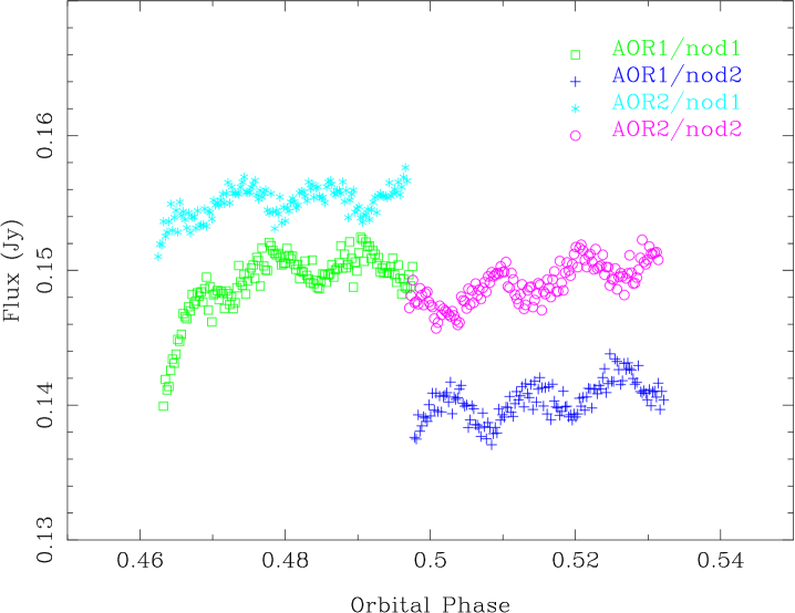
Figure 1: The 9 $\mu$m flux time series for AOR 14817792 and AOR 14818048. In both AORs, a nod was executed near the center of the secondary eclipse period. The measured flux is affected by systematic errors caused by (i) pointing, (ii) background subtraction, and (iii) latent charge accumulation; these effects combine to cause changes in the measured flux that are $\sim$10x larger than the secondary eclipse signature. The pointing error causes the offset between the flux density in the nod 1 data in both AORs, and it causes most of the offset in flux density between the nod 1 and nod 2 data for a given AOR; the pointing error also causes the linear and periodic changes in the measured flux. The background subtraction error causes a portion of the offset between the nod 1 and nod 2 data for a given AOR. The latent charge accumulation error causes the initial rapid increase in measured flux; this effect is larger in AOR 14817792 due to the array history.

The observations we analyzed (originally proposed by Richardson et al. 2007) were taken with the Spitzer Space Telescope (Werner et al., 2004) using the Infrared Spectrograph (IRS; Houck et al. 2004). The data were taken on 6 July 2005 and 13 July 2005 as two separate Astronomical Observing Requests (AORs 14817792 and 14818048) and provide approximately continuous coverage of the secondary eclipse event (see Fig. 1). The timing of the observations is well suited for application of the secondary eclipse technique (also termed “occultation spectroscopy”), in which data from portions of the orbit where light originates from the “star+planet” and “star” are subtracted to obtain the planet’s emission (Richardson et al., 2003). For both sets of observations, the IRS instrument was operated in first order (7.5 to 15.2 $\mu$m) at low spectral resolution (R=60-120; SL1) with a nod executed at the midpoint of the observations. This observational sequence provides two completely independent data sets that span an interval covering the sequence:

1. before eclipse (flux originates from star+planet),

2. ingress (planet flux contribution changing with time),

3. secondary eclipse (flux originates from star only),

4. egress (planet flux contribution changing with time), and

5. after eclipse (flux originates from star+planet).

Each nod contains 140 samples with an integration time of 60 seconds each.

To determine the orbital phase of HD 209458b we used the results by Knutson et al. (2007) for both the period and the ephemeris. The time for each data point was determined using the $\rm DATE\_OBS$ keyword in the header, which was then converted to Julian date using the IDL routine JDCNV.pro from the IDL astronomy library. We then converted to heliocentric Julian date (HJD) using the IDL routine $\rm HELIO\_JD.pro$ (also from the astronomical library) for direct comparison with the Knutson et al. (2007) results. The phase was then estimated by $phase=((time\_in\_HJD-ephemeris)\times mod(period))/period$. In what follows, we will refer to the segment of the orbital phase when both star and planet are visible as “SP”. Similarly, we refer to the segment of orbital phase when only the star is visible (when the planet is passing behind the star) as “S”. To determine the planet spectrum, we have applied the analysis described below to the spectral range of the IRS SL1 module.

3 Analysis

The extracted flux density time series suffers from four kinds of temporal changes (see Fig. 1) that completely dominate (by a factor of $\sim$10) the expected signature of secondary eclipse flux decrement of $\sim$0.0025 (Deming et al., 2005a). These effects are (i) a flux offset between nods, (ii) a periodic flux modulation, (iii) initial flux stabilization, and (iv) monotonic flux drift within a nod. These temporal changes are not random; a scatter diagram shows that the flux density values are highly correlated (correlation coefficients of $\sim$0.99). We find that these four major temporal flux density changes listed above are caused by (in order of importance) errors in telescope pointing, background subtraction, and latent charge accumulation.

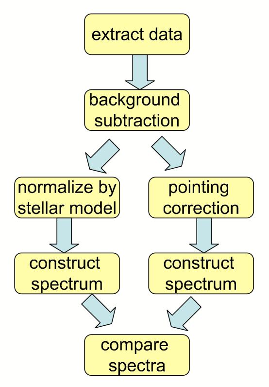
Figure 2: A schematic representation of the steps in our data reduction procedure; a detailed discussion of each stage of this process is contained in the text. The strength of this approach is that it provides two semi-independent methods of estimating the planet spectrum. Because the two methods interact with systematic errors differently, the comparison of the results provides a robust method for demonstrating control of these errors. In the final step of the data reduction, the estimates of the planet spectra from the two methods are compared.

Effective calibration of these systematic effects can be challenging to demonstrate. To test our control of the systematic errors, we developed two methods for estimating the exoplanet spectrum. The first method is differential and has the property that errors which are “common-mode” in wavelength are rejected. The second method is an absolute method and results in an exoplanet spectrum in units of Jy. A schematic picture of our data reduction method is shown in Fig. 2; central to our approach is comparing the results of the two semi-independent estimates of the exoplanet spectrum. Because the two methods interact with systematic errors differently, the comparison is useful for accessing the level of uncalibrated, residual systematics. In this section, we describe the initial data extraction, the major systematic errors, and each of our spectral extraction methods. In Section 4, we discuss the comparison between the differential and absolute methods for obtaining the planet spectrum. We then present our results and discuss the implications. We also discuss the differences between the methods and results of our approach and previous work.

3.1 Data Extraction

Our initial data extraction method is an extension of the method described by Bouwman et al. (2006). The series of extracted images are used to define a median background image for each of the two nod positions. The median background image (for each nod position) is then subtracted from all the individual observations with the source in the other nod position; this generates the background subtracted images. We then identify bad pixels using a median filter and visual inspection. The bad pixels are then corrected using an approach similar to the Nagamo-Matsuyama filtering method (Nagano & Matsuyama, 1979). The source spectrum is then extracted using the method developed by Higdon et al. (2004) and implemented in the SMART data reduction package.

The spectra were extracted using a fixed-width aperture of 6 pixels centered on the position of the source. The exact source position relative to the slit was determined by fitting a $sinc$ profile to the spectra in the dispersion direction using the collapsed and normalized source profile. The accuracy at which the source position can be determined is about 0.02 pixels. This, together with the aperture width of 6 pixels, ensures that any flux variablity due to slight changes in the positioning of the aperture are far less than the expected planetary flux.

3.2 Systematic Errors

Here we discuss the origin and chromaticity of the three significant systematic errors present in these data. There may be other systematic errors as well, but they, and the residuals of the errors we explicitly deal with, are smaller than the uncertainty level achieved in our calibration. We acknowledge that there are different points of view regarding the calibration of IRS data for determining exoplanet spectra (Richardson et al., 2007; Grillmair et al., 2007) and that these approaches may perform similar (but not identical) corrections to the data while ascribing the underlying systematics to different causes. However, ours is the only method that allows determining the absolute planet spectrum.

3.2.1 Pointing Errors

The periodic and linear drift components of the Spitzer pointing error have been documented with long-duration IRAC observations (Morales-Calderón et al., 2006). Pointing errors cause modulation of the measured flux because telescope motion perpendicular to the slit axis changes the position of the stellar image with respect to the spectrometer entrance slit; this causes changes in the vignetting of the stellar image. Even small pointing errors change how the wings of the point spread function (PSF) are vignetted. Since the PSF size is proportional to wavelength, the measured flux changes due to pointing are wavelength dependent. In the absence of other effects, the measured flux density, $S(\lambda)$, is

$$S(\lambda)={\bf\zeta}(y,\lambda)F(\lambda)$$ (1)

where $F$ is the “true” flux density, $\zeta$ is the pointing-induced fractional flux density ($\zeta=1$ for no pointing error), and $y$ is the angular error with respect to the spectrometer entrance slit center position in units of pixels. In principle, if $\zeta$ can be determined, the effects of pointing error can corrected.

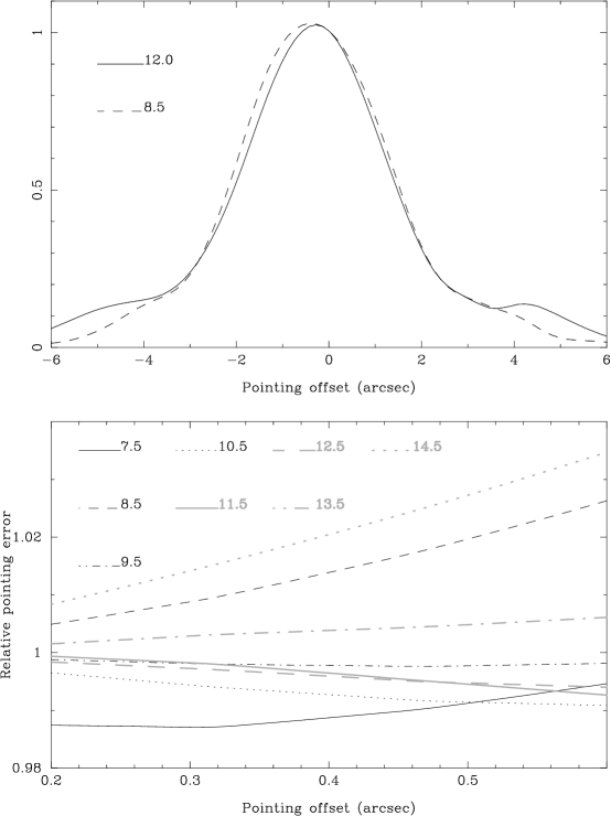
Figure 4: Top: The change in measured flux as a function of source position in the cross-slit direction of the IRS entrance slit. This calibration was developed from slit scans of IRS calibrators (see text). The measured flux does not peak at zero offset because of an asymmetry in the wings of the PSF. Given the 0.4 arcsecond radius of the IRS “high precision” peakup mode error circle, the uncertainty associated with the standard IRS high-precision peakup results in a $\sim$ 7 % uncertainty in the measured flux. The measured flux error due to the cross-slit pointing error is, to first order, common mode in wavelength. Bottom: The pointing offset correction as a function of wavelength normalized to 12 $\mu$m. This plot shows that there is a spectral error of $\sim$ 1.5 % across the instrument passband due to the pointing offset effect for the standard high-precision peakup. The horizontal scale is set to include the range of offsets present in the observations of HD 209458.

We determined $\zeta(y,\lambda)$, by using the spectral map observations of IRS calibrators HD 173511 (AOR 13481216) and HR 7341 (AOR 16295168). The spectral map data consist of a series of pointed observations in which the star spectrum is measured on a two-dimensional grid (7x7 and 5x23 positions, respectively, for these AORs). For each scan perpendicular to the slit axis, we normalized the measured spectrum by the spectrum measured at the nominal slit center position, $\zeta(y)=S_{y}/S_{0}$. Assuming the slit has a constant width, we combined the normalized measurements from all the slit scans. This resulted in a series of values at each nominal pointing position perpendicular to the slit axis ($y\in[y_{1},y_{2},y_{3},\ldots]$). The difference in these values at each nominal slit scan position reflects a pointing error that can be corrected for in an iterative process. We defined a “template” by taking the average value of the points at each pointing offset position. The individual slit scan data were then shifted in the horizontal axis and renormalized to minimize the $\chi^{2}$ value of the shifted curve with respect to the template. After all the slit scans had been shifted and renormalized, a linear interpolation was done to find revised values for the template function at the nominal pointing offset positions transverse to the slit axis. The individual slit scan data were then shifted and renormalized again for a best fit to the revised template function. This process was iterated until convergence was reached; it resulted in pointing-error-corrected, slit-scanned data. We determined $\zeta$ by fitting a cubic-spline at each wavelength through the shifted and renormalized slit scan measurements (see Fig. 4 top).

While a periodic pointing error component is frequently seen in Spitzer observations, it is not necessarily repeatable in terms of shape or amplitude (Carey, 2007). The IRS data we analyzed for HD 209458 show a periodic modulation of the measured flux (see Fig. 1) that could be due to the Spitzer pointing error. To test the hypothesis that changes in the measured flux are due to pointing errors, we modelled the pointing error periodic motion in both the spatial and spectral axis. This leads to an elliptical motion that creates a symmetric profile about individual maxima and minima. The asymmetric profiles in these data require the addition of a harmonic term for angular velocity; when this is incorporated, the pointing error is given by

$$\dot{\theta}=\dot{\theta_{0}}+A_{\theta}sin(\omega t-\phi_{\theta}),$$ (2)

$$x=x_{o}+m_{x}t+A_{x}cos[\omega\theta(t)-\phi_{x}],$$ (3)

$$y=y_{o}+m_{y}t+A_{y}cos[\omega\theta(t)-\phi_{y}],$$ (4)

where $t$ is time, $x$ is the position parallel to the slit axis (the spatial dimension on the array), $y$ is the position perpendicular to the slit axis (the spectral dimension of the array), $x_{o}$ and $y_{o}$ are initial offsets, $m_{x}$ and $m_{y}$ are the linear drift terms, $\dot{\theta}$ is the angular velocity, $A$ is the amplitude, $\omega$ is the frequency, and $\phi$ is the phase. The normalization of $t$ and $\dot{\theta}$ is determined by the conditions

$$t\in[0,2\pi],\int_{0}^{2\pi}\dot{\theta}dt=2\pi,A_{\theta}\leq\dot{\theta_{0}}.$$ (5)

We determined the parameters for the $x$ and $\theta$ components of our pointing model by fitting to the source motion along the slit axis using the following steps for the data in each AOR:

1. Determine position: For each measurement in the time series, we constructed the spatial profile at each spectral channel. These profiles are normalized by wavelength in the spatial axis and shifted so that they can be “stacked” coherently. A median spatial profile is then determined. This median spatial profile is then fit with the function $sinc^{2}(x)$. The fitted position of the maximum of $sinc^{2}(x)$ as a function of time is used as the measure of telescope pointing changes in the spatial axis.

2. Linear fit: We fit and removed the linear component, $m_{x}$, of the source position in the spatial axis of the data in each nod.

3. Determine the frequency: To determine the frequency, $\omega$, of the periodic oscillation in each nod, we took the Fourier transform of the linearly detrended position function in the slit spatial axis. The normalized frequency values were the same within the errors, and the mean frequency was used in the remaining analysis.

4. Characteristic profile: We folded the data, computed a median profile and local standard deviation, applied a 10 $\sigma$ clip to remove discrepant points, and determined the mean profile.

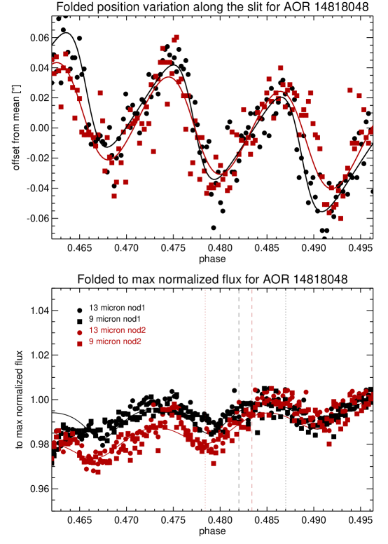
Figure 3: Top: Source position data in the slit spatial axis, together with an elliptical pointing model for AOR 14818048. Both periodic motion and a linear drift are clearly identifiable in the source position data. The data are fit to determine the amplitude, period, eccentricity, and linear drift terms. After determining the best fit pointing model using the data in the spatial axis, we investigated the effect of the cross-slit motion predicted by this model. Bottom: The normalized cross-slit projected motion from the elliptical pointing model as a function of time; with the exception of the initial few points, the excellent agreement between the model and the data is evident. This strongly suggests that time-variable pointing errors (periodic changes and linear drifts) are primarily responsible for changing the measured flux.

5. Determine model parameters: We determine the values for $x_{o},A_{\theta}$, $A_{x}$, $\phi_{\theta}$, $\phi_{x}$ by fitting the predicted position along the slit axis to the measured source position along the slit axis (see Fig. 3); the values for these parameters are given in Table 1.

At this point, we only need to determine the values of $(y_{0},m_{y},A_{y},\phi_{y})$ to completely describe the telescope pointing. Judicious selection of values for $(y_{0},m_{y},A_{y},\phi_{y})$ produces an estimate of the cross-slit position changes that (with appropriate normalization) agree remarkably well with the intensity time series (see Fig. 3 bottom) and successfully reproduce the asymmetric component in the shape of the periodic modulation.

The excellent agreement between our simple pointing model and the observed changes in the measured flux confirm that, in the case of a point source, the IRS measurement of the flux density is affected by the position of the (stellar) image in the spectrometer entrance slit. The results (see Fig. 3 bottom) imply that pointing changes as small as $\sim$ 10 milliarcseconds have an effect on the measured IRS flux for bright, point-like objects. Because the PSF size is a function of wavelength, the pointing error effect is chromatic. The asymmetry in the PSF wings also causes pointing errors to be asymmetric with respect to the nominal center of the slit (this can be seen in Fig. 4).

Equipped with equations 1 and 4, we can now decompose the changes in the measured flux density into three specific kinds of pointing errors, all of which can be seen in Fig. 1. Each of these pointing errors contributes a specific component of $y$. Note that the values of $A_{y}$ & $\phi_{y}$ are the same for all AOR/nod combinations, while $y_{o}$ & $m_{y}$ are different for each AOR/nod combination.

• initial peakup/nod error - The pointing error associated with the initial peakup or nod operation. The high-accuracy peakup, used for these observations, has a 1-$\sigma$ error circle radius of 0.4 arcseconds. This translates into a flux uncertainty of $\sim 5-10$%. When a nod is executed, there is significant motion perpendicular to the slit axis. This is the reason why the median flux density differs in each AOR/nod1. The initial error is static and represents a constant offset described by $y=f(y_{0})$.

• pointing drift - During an observation, there is a slow linear drift in pointing during each nod. The drift rate is larger at the nod2 position. The slow pointing drift rate ranges from 3 mas/hr to 19 mas/hr (based on a 1.85 arcsecond per pixel plate scale and a nod duration of 2.9026 hr - see Tab. 1). This linear pointing error is described by $y=f(m_{y})$.

• periodic error - The Spitzer telescope has a known periodic pointing error $\sim\pm 30$ milliarcseconds. This is the error that causes the clear periodic modulation of the flux. The periodic position changes are described by $y=f(A_{y},\phi_{y})$.

3.2.2 Background Correction

In the mid-infrared, accurate measurement of the infrared source flux requires subtraction of the background due to local zodiacal emission. To remove the background contribution to the spectrum, we construct and subtract a median background image. However, this median image must be constructed with care as there is a systematic error in the backgound estimate due to leakage from the bright source. This leakage is manifested as a flux density offset between the background at the nod1 and nod2 positions. In principle, this offset could be caused by structure in the background. However, inspection of IRS calibrator star data shows that the difference in the background between the nods is systematic in that it occurs for all the multiply observed IRS calibrators we checked; the effect is highly repeatable and is proportional to the measured source flux. IRS calibrators observed with a series of slit offsets show the measured source flux decreases with the slit offset from the target, and the background offset is proportional to the measured flux. This suggests that some of the light from the source contaminates the background through the wings of the PSF. Because the Spitzer PSF is asymmetric (Bayard & Burgarolas, 2004), the leakage differs in nod 1 and nod 2.

To determine the amount of a point source contamination in the background estimate, we have used observations covering an interval of approximately three years for five IRS calibrator stars (HR 6606, HR 7341, HD 166780, HD 173511, HR 6348), together with the assumption of a locally uniform background. The IRS calibrators we selected were observed in the nominal nod1 and nod2 positions for both SL1 and SL2 modes. These stars were observed on a regular basis throughout the Spitzer operational period up to the time of these observations. Each star was typically observed at least 20 times over a three year interval. Thus, slit precession over a period of one year is a strong test of our assumption of uniform background.

We determined the source contamination in the background by subtracting two SL1 background positions when the star is in the SL1 and SL2 positions. The background source contribution function, $BSCF$, for the nod1 position has the form

$$BSCF_{nod1}=\frac{S_{leak}(nod1)}{S_{source}(nod2)}=\frac{B_{nod1}(SL1,nod2)-B_{nod1}(SL2,nod1)}{S^{\prime}(nod2)-B_{nod2}(SL2,nod1)}\left(\frac{RSRF_{nod2}}{RSRF_{nod1}}\right),$$ (6)

where $B_{nod1}(SL1,nod2)$ is the background at the nod1 position measured when the source is located at the SL1, nod2 position; $B_{nod1}(SL2,nod1)$ is the background at the nod1 position measured when the source is located at the SL2, nod2 position; $S^{\prime}(nod2)$ is the measured source flux at the SL1, nod2 position with no background correction; and $RSRF$ is the relative spectral response function at either the nod1 or nod2 source position. For each term, the subscript denotes the position on the array where the value was measured while the source position at the time of the measurement is indicated by the parenthesis. Thus, $B_{nod1}(SL2,nod1)$ is the background measured at the SL1, nod1 position when the source is located at the SL2, nod1 position. Since we are calibrating SL1 data, the background is always measured in the SL1 slit. However, determining the $BSCF$ requires using data when a star was observed with both the SL1 and SL2 slits. The $BSCF_{nod2}$ is similarly defined except that all nod1 instances become nod2 and visa versa. The corrected background flux density at the two SL1 nod positions is then

$$S(nod1)=\left[S^{\prime}(nod1)-B_{nod1}(SL1,nod2)\right]+BSCF_{nod1}\times S(nod2),$$ (7)

and

$$S(nod2)=\left[S^{\prime}(nod2)-B_{nod2}(SL1,nod1)\right]+BSCF_{nod2}\times S(nod1).$$ (8)

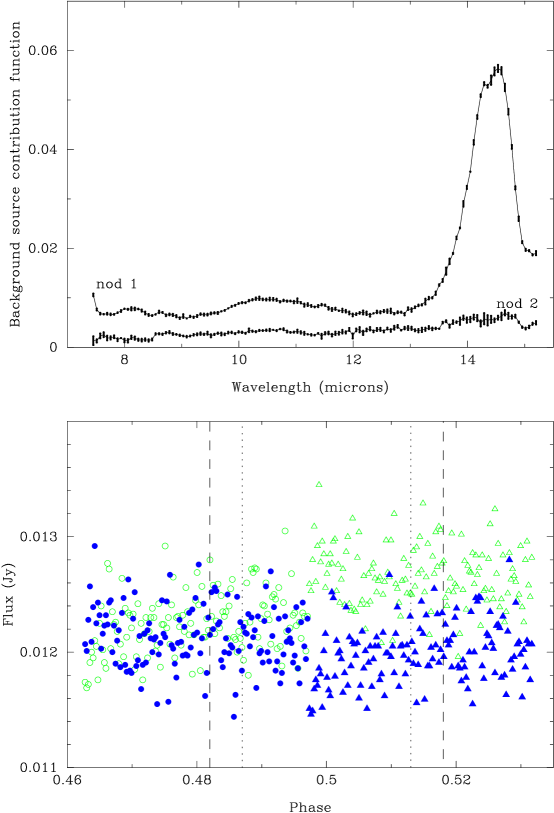
Figure 5: Top: The background source contribution function (BSCF) is different for the two nods because of an asymmetry in the telescope PSF (see text for description of the derivation). Multiple stars and epochs were used to determine both the correction and the uncertainty. Bottom: The open circles (nod1 background) and triangles (nod2 background) are the estimated background prior to correction for the source contribution at 12 $\mu$m in AOR 14818048. The filled circles and triangles show the result of applying the correction for source leakage.

The system of linear equations is then solved for the background corrected, measured source flux density, $S$, at each nod position. This results in an estimate of the $BSCF$ each time the calibrator stars were observed. We then averaged the results for all the calibrator observations to determine a mean $BSCF$ (see Fig. 5). The uncertainty in the $BSCF$ at each wavelength was determined by the standard deviation in the mean.

Applying the $BSCF$ substantially reduces the background flux density offset between the nod1 and nod2 positions (see Fig. 5). For wavelengths shorter than 13 $\mu$m, the correction we derive is $\sim$0.4% for nod 1 and $\sim$0.9% for nod 2. This means that there can be $\sim$ 0.5% of the source flux present in the wings of the PSF $\sim$ 20 arcseconds away from the observed source position. Thus, the contamination of the background by the source is of the same magnitude as the signal from the exoplanet. This correction for source contamination of the background may not be necessary for many observations. However, for high dynamic range measurements on bright point sources, neglecting the leakage of the source into the background estimate introduces systematic errors in the data for each nod.

3.2.3 Latent Charge Accumulation

In the context of the IRS instrument, latent charge accumulation has been reported by several authors (Grillmair et al., 2007; Richardson et al., 2007; Deming et al., 2006), and is sometimes termed “charge trapping”. Currently, the details of the semi-conductor physics that produce the effect are not well understood. Empirically, the responsivity of a pixel initially depends on the illumination. When the flux density time series is median-normalised (e.g. $F_{i}(\lambda)/<F(\lambda)>$), the light curves at each wavelength can be “stacked” (Richardson et al., 2007). The effect of latent charge accumulation can be seen at the beginning of each AOR in Fig. 1; the effect is characterized by a rapid initial increase in the measured flux density, which then approaches an equilibrium. If one excludes the first $\sim$ 20 points in each AOR and finds the slope of a best fit line to the data, the slope in nod2 is greater than the slope in nod1. As Fig. 3 shows, a simple pointing model explains the changes in the measured flux after the first $\sim$ 20 minutes. Note that it is possible to confuse the linear component of the pointing drift with the effect of latent charge accumulation after the first $\sim$ 20 minutes. By explicitly modelling the pointing, our analysis breaks this degeneracy and allows us to separate the effects of these two systematic errors. We conclude that latent charge effects are negligible after the first 20 minutes. We omitted the data affected by latent charge accumulation from further analysis so that the effects of latent charge do not impact our estimate of the planet spectrum.

3.3 Spectral Response Function

After the initial extraction, the data were background corrected using the background correction discussed above. The next stage of the calibration was to derive and apply a spectral response function. Using the IRS calibrator $\eta$ Dor, we derived our own spectral response function, the $SRF$, for the nominal nod positions and extraction aperture. We selected this source for defining the spectral response function because it has the same brightness as HD 209458 and thus should minimize any remaining instrument residuals. Both HD 209458 and the $\eta$ Dor data were extracted using identical methods, and both incorporate identical methods for background correction. Thus, the treatment of both the calibrator and source data sets is fully self-consistent. In the case of AOR 14818048, an additional calibration step for the $SRF$ was required because the observations were not carried out at the nominal nod positions. To determine the changes in the $SRF$ for other (but still relatively nearby slit positions), we used observations of the IRS calibrator stars HD 42525 and HR 7341, which were observed at intervals along the IRS slit. We interpolated between observing positions to determine how the calibrator star’s spectrum changed as a function of slit position and used this information to renormalize the $SRF$ derived, using $\eta$ Dor for the nod positions used in AOR 14818048.

At this point, the data were ready for extraction of the spectrum. Of the three major systematic errors, the background had been removed (at this point in the calibration sequence) by explicit calibration. The effects of latent charge were removed by excluding the effected data from the spectral estimation. However, the pointing error remained uncorrected. In what follows, two methods were used to correct the pointing error and extract the planet spectrum.

3.4 Spectral Estimation

3.4.1 Differential Method

This approach assumes that changes in the measured flux have a wavelength-independent component, characterized by $G(t)$, which can vary on a timescale of minutes, and a wavelength-dependent component, $G(\lambda)$, which is stable for a given nod but can change between nods. The $G(\lambda)$ term is removed by construction of a spectral flat. We derived a spectral flat for each nod by comparing the average flux in each spectral channel to the flux, $F(\lambda)$, of a stellar photosphere model for HD 209458 (Kurucz, 1992) normalized to the 12 $\mu$m flux. Thus at each wavelength, $\lambda$, the spectral flat was defined as the inverse of $[S_{S}(\lambda)/F_{Kurucz}(\lambda)]\times[F_{Kurucz}(12)/S_{S}(12)]$ where $S_{S}$ is the measured flux observed in interval S. After normalization of each nod by the associated spectral flat field, the data were assumed to vary only in time; a more extensive discussion of this technique can be found in Bryden et al. (2006) and Beichman et al. (2006). To reject the wavelength-independent $G(t)$ term, we constructed a differential observable using the following method. During period SP (star+planet), the measured flux, $S_{SP}(\lambda)$, can be written as

$$S_{SP}(\lambda)=G(t)\left[F_{S}(\lambda)+F_{P}(\lambda)\right].$$ (9)

This can be expanded as

$$S_{SP}(\lambda)=G(t)F_{S}(\lambda)\left[1+\frac{F_{P}(\lambda)}{F_{P}(\lambda^{{}^{\prime}})}\frac{F_{P}(\lambda^{{}^{\prime}})}{F_{S}(\lambda^{{}^{\prime}})}\frac{F_{S}(\lambda^{{}^{\prime}})}{F_{S}(\lambda)}\right],$$ (10)

where $F(\lambda)$ is the true source flux, the subscripts refer to the star or planet, and $\lambda^{{}^{\prime}}$ is a reference wavelength selected for the comparison. We set the transit depth at $\lambda^{{}^{\prime}}$ to a plausible value such that $\beta=(F_{P}(\lambda^{{}^{\prime}})/F_{S}(\lambda^{{}^{\prime}}))<<1$ and the transit depth at $\lambda$, relative to the transit depth at $\lambda^{{}^{\prime}}$, is $\alpha=(F_{P}(\lambda)/F_{P}(\lambda^{{}^{\prime}}))$. $S_{SP}(\lambda)$ can then be expressed in terms of $\alpha$ and $\beta$ as

$$S_{SP}(\lambda)=G(t)F_{S}(\lambda)\left[1+\alpha\beta\frac{F_{S}(\lambda^{{}^{\prime}})}{F_{S}(\lambda)}\right].$$ (11)

During period S (star only), the measured signal, $S_{S}$, is $S_{S}(\lambda)=G(t)F_{S}(\lambda)$. The ratio of the two wavelengths during the SP and S periods is $R_{SP}=S_{SP}(\lambda)/S_{SP}(\lambda^{{}^{\prime}})$ and $R_{S}=S_{S}(\lambda)/S_{S}(\lambda^{{}^{\prime}})$. The advantage of taking the ratio is that the wavelength-independent gain term, $G(t)$, drops out. Appropriate substitution, and solving for $\alpha$, yields

$$\alpha=[R_{SP}(1+\beta)-R_{S}]/\beta.$$ (12)

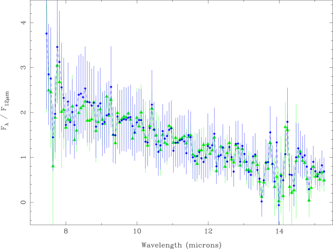
Figure 10: The mid-infrared spectrum of HD 209458b derived using the absolute method (circles) and the wavelength differential method (triangles). For both cases, the spectrum has been normalized to the 12 $\mu$m flux and scaled so that the average flux for both plots is identical. While the agreement is excellent over most of the passband, the effect of small, uncorrected pointing errors causes the differential spectrum to lie slightly below the absolute spectrum at some wavelenghts between 7.5 and 9 $\mu$m.

The observables are $R_{SP}$ and $R_{S}$, and $\alpha$ is the measure of the brightness of the planet at $\lambda$ compared to the planet brightness at $\lambda^{{}^{\prime}}$. The results in Fig. 10 reflect a value for $\beta=0.003$. However, the results for the spectral slope are not strongly dependent on the assumed value for $\beta$, and we explicitly measured the eclipse depth in any case (using the absolute method).

We summarize the steps in the differential method as follows:

1. Treat each AOR and nod combination as an independent secondary eclipse measurement with an independent calibration; this leads to four independent estimates of the planet spectrum.

2. Normalize the data in a given nod by dividing the flux density by the 12 $\mu$m value at each sample in the time series.

3. Average the SP and S intervals in the time series to get the “star only” and “star+planet” spectra.

4. Normalize a Kurucz model for HD 209458 flux density by the model’s 12 $\mu$m prediction.

5. Construct a “super flat” by dividing the normalized Kurucz model into the normalized data (for both SP and S intervals).

6. Estimate the planet spectrum by subtracting the S interval spectrum from the SP interval spectrum.

The four estimates of the exoplanet spectrum are then averaged to create the final spectrum. The errors are estimated by taking the average value of the differences in the estimate at each wavelength.

To assess the magnitude of residual systematics, we made a comparison (see Fig. 10) between the spectra from each of the four independent AOR and nod combinations. In the central region of the IRS SL1 instrument bandpass, the spectra are in relatively good agreement. However, this agreement becomes worse at either end of the instrument bandpass; this is especially true for wavelengths between 7.5 and 9 $\mu$m. The reason for this is that the assumption that $G(\lambda)$ is time invariant is only a first order approximation. Because we have normalized by the 12 $\mu$m flux density, the effect of the small, uncorrected pointing errors within a nod is greatest at the band edges (see Fig. 4). To determine the best estimate of the differential spectrum, the four independent differential spectra are averaged together.

3.4.2 Absolute Method:

Here we describe how to apply the $\zeta$ correction to the source and calibrator data. Although we do not know a priori what the telescope pointing error is, we can determine the correct flux density for a given pointing error, $y$, using $F=S/\zeta(y)$. From Eq. 4, we know that $y=f(y_{0},m_{y},A_{y},\phi_{y})$. Thus, our task is to identify the correct values for ${y_{0},m_{y},A_{y},\phi_{y}}$. One way to do this is to require that the absolute spectrum be self-similar. We implemented this by constructing all unique combinations of the relation

$${\bf R(i,j)}=F_{i}(\lambda,\theta)/F_{j}(\lambda,\theta)=\frac{S(t_{i})\zeta(y_{j})}{S(t_{j})\zeta(y_{i})}$$ (13)

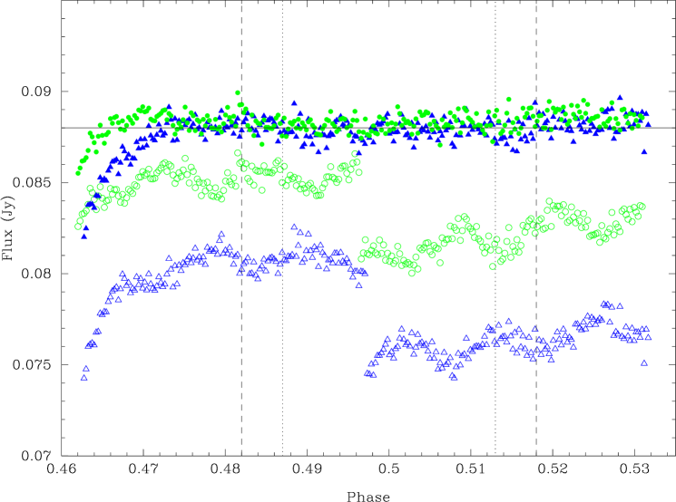
Figure 7: The 12 $\mu$m flux time series for AOR 14817792 and 14818048 as a function of orbital phase. The background-subtracted data are shown in open circles and triangles. The large discontinuity halfway through each data set corresponds to a nod; periodic changes and drifts also affect the time series measurements. The changes in measured flux are primarily due to telescope pointing errors, which cause variable vignetting by the spectrometer entrance slit of the wings of the source point spread function. The filled points show the pointing-corrected flux. The signature of the secondary eclipse is visible as an interval with systematically lower flux density. The vertical dashed lines indicate the region of ingress/egress where the planet is partially obscured by the star. A horizontal line has been added to aid in identifying the flux density decrease during secondary eclipse. Note that the effect of latent charge accumulation can be seen in the apparently increasing flux in the initial $\sim$ 20 points for each AOR (near orbital phase 0.464).

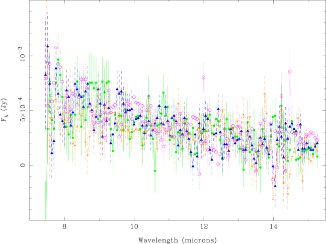
Figure 8: Four independent estimates (nod1 and nod2 for both AOR 14817792 and AOR 14818048) of the planet spectrum, determined using the absolute method, are plotted together as an internal consistency check. The internal agreement of the absolute method is excellent over the entire instrument passband.

for the SP and S portions of each nod separately, where $i$ and $j$ are individual measurements in the time series. We then iteratively searched this space to determine the values of ${y_{0},m_{y},A_{y},\phi_{y}}$ (given in Tab. 2), which resulted in most closely approximating ${\bf R(i,j)}=1$. Fig. 7 shows the result of the application of the pointing offset correction, and the secondary eclipse event is directly visible. Similarly, we applied the $\zeta$ correction to $\eta$ Dor and determinded the pointing offset by requiring spectral self-similarity. As with the differential method, we evaluated the internal consistency of the pointing correction by comparing the spectra from both nods in both AORs. The agreement between the absolute spectra is excellent (see Fig. 8), and we now compare the differential and absolute spectra to assess the level of any residual systematics.

4 Discussion

In this section, we compare the results of the differential and absolute methods we used to extract the planet spectrum. The assumption of wavelength-dependent stability used in the differential method is evaluated. We discuss our estimate of the eclipse depth and spectral features; we interpret these results in the context of recent models. We also discuss the significant differences between our analysis methods and results and those of Richardson et al. (2007).

4.1 Comparison of differential and absolute methods

A fundamental strength of our approach is the use of two semi-independent methods to demonstrate understanding and calibration of the dominant systematic errors. As Fig. 10 shows, the agreement between the differential and absolute planet spectrum estimation methods is excellent over most of the instrument passband. While agreeing within the errors, between 7.5 and 9 $\mu$m, the differential spectrum is systematically below the absolute spectrum. This is caused by small pointing errors occuring within a nod that are not removed by the differential method. Because the internal scatter of the absolute method is similar at all wavelengths, we consider the absolute spectra to be the best estimte of the planet spectrum.

That the two spectral extraction procedures yield consistent results is encouraging and gives us a high degree of confidence that the calibration of systematic errors is successful within the error bars. Given that the differential method appears to make no specific correction for pointing, one might wonder why the agreement with the absolute method is so good. The source of the agreement is that the normalization by the Kurucz model corrects for any chromatic error, pointing or otherwise, so long as the chromatic error changes in time are relatively small. Thus, normalization by the Kurucz model corrects the chromatic error produced by the largest pointing errors, which are static and occur during the initial peak-up and during the nod. Because the periodic pointing errors are relatively small, the change in the measured flux during a nod is, to first order, wavelength independent, and thus the spectral flat field is a good approximation for the flux correction due to the initial pointing error. Thus, the agreement between the differential and absolute spectral estimation methods supports the original assumption that the $G(\lambda)$ term is relatively (but not completely) constant during a nod. The increased size of the error bars in the differential method results from the periodic component of the pointing errors.

4.2 Eclipse Depth

We have determined an average eclipse depth for the data by normalizing the absolute (pointing error corrected) flux density time series at each wavelength by the median values of the time series, $F(\lambda)/<F(\lambda)>$. This is then averaged over wavelength to develop a broad-band light curve. The result of this can be seen in Fig. 9; the broad-band light curve clearly shows the eclipse and the transitions between ingress and egress. We can derive four independent estimates (one for each nod) of the broad-band eclipse depth, and these are consistent within the errors. After averaging the individual estimates, we find the average eclipse depth between 7.6 and 14 $\mu$m to be 0.00315$\pm$0.000315. This minor restriction in wavelength was implemented to exclude the channels with lower SNR. When compared to theoretical models (Burrows et al., 2006), the measured eclipse depth suggests that substantial heat redistribution from the dayside to the nightside is occurring. This evidence of heat redistribution is similar to the interpretation given to observations of HD 189733b by Grillmair et al. (2007) and Knutson et al. (2007).

4.3 Planet Spectrum

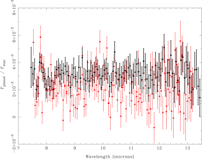
Figure 12: The contrast spectrum for HD 209458b as determined by our calibration method (black circles) and the method used by Richardson et al. (2007) (red triangles). Over the range of wavelengths where the spectra can be directly compared, the internal scatter of our spectrum is 2.3 times smaller than the previous result. The methods are in qualitative agreement, and both show evidence for modulation of the spectrum between 7.5 and 8.5 $\mu$m. This modulation includes a broad feature seen as a local minima centered at approximately 8.1 $\mu$m, and a narrow feature that could be either a local minima at approximately 7.57 $\mu$m or a local maxima centered at approximately 7.63 $\mu$m.

We have determined the planet spectrum (see Fig. 11) and find it to range from about 600 $\mu$Jy at 7.5 $\mu$m to about 200 $\mu$Jy at 15.2 $\mu$. The SNR in the spectrum ranges from $\sim$ 10 at short wavelengths to $\sim$ 2 at the longest wavelengths. To our knowledge, this is the first determination of the absolute spectrum of exoplanet emission. Our results for the spectral shape agree well with previous work (see Fig. 12) albeit with improved SNR; specifically, we confirm the marginal detection by Richardson et al. (2007) of a narrow feature near 7.7 $\mu$m. For most wavelengths, the planet spectrum is characterized by approximately featureless emission. However, between 7.5 and 8.5 $\mu$m, there is evidence for one broad (previously unreported) and one narrow (previously reported) spectral feature.

Both the absolute spectrum and the contrast spectrum show evidence of a possible $\sim$ 0.5 $\mu$m-wide feature centered around 8.1 $\mu$m, with a significance of about 4 $\sigma$. This broad feature represents a flux deficit from the local trend and could be due to absorption. At the full spectral resolution, there is also a suggestion of a narrow feature around 7.7 $\mu$m. This narrow feature candidate could be either in absorption (a deficit relative to the local trend in the 7.57 and 7.63 $\mu$m channels) or in emission (an excess relative to the local trend in the 7.69 and 7.75 $\mu$m channels). The shape of the broad feature causes us to favor the hypothesis of a narrow absorption feature in the 7.57 and 7.63 $\mu$m channels. However, movement of any one of these four spectral points (7.57, 7.63, 7.69, and 7.75 $\mu$m) by $\sim$1.5 $\sigma$ towards the local trend would convert this candidate feature into an outlier consistent with a normal measurement distribution. The narrow feature candidate is sufficiently marginal that additional observations are required to confirm or rule out a spectral feature at this wavelength.

The indication that the spectrum of HD 209458b contains one broad and one narrow feature between 7.5 and 8.5 $\mu$m is supported by the Richardson et al. (2007) measured spectrum. Indeed, the striking qualitative agreement (one broad and one narrow feature) between previous work and our results for the spectral modulation between 7.5 and 8.5 $\mu$m is a strong indication that this modulation is real. Although Richardson et al. (2007) did not discuss the broad feature, it is present in their spectrum and we confirm their measurement. While we cannot totally exclude the possibility of some residual instrument systematic, it is highly significant that the shape of this spectral modulation is consistent using three independent methods conducted by two independent groups. Because of the repeatability of the result and the maturity of the exoplanet spectrum determination, the spectral modulation between 7.5 and 8.5 $\mu$m is likely real and may serve as a useful constraint on models for emission from HD 209458b.

In the interpretation of the previous results for these data, Richardson et al. (2007) reported the detection of a broad emission feature centered at 9.65 $\mu$m, identified as a silicate feature, and a narrow emission feature centered at 7.78 $\mu$m. We find no evidence to support the identification of a 9.65 $\mu$m feature in our spectrum. Additional averaging and scrolling median filtering does not reveal any candidate feature with the characteristics claimed by Richardson et al. (2007). It is possible that the narrow feature identified by Richardson et al. (2007) corresponds to the 7.67 and 7.75 $\mu$m channels in our analysis. If this is the case, the difference in wavelength is possibly due to the non-standard wavelength calibration method used by Richardson et al. (2007) (see discussion below). However, we stress that the candidate absorption feature at 7.57 $\mu$m is at least as likely as an emission feature at 7.69 $\mu$m

4.4 Differences with Previous Work

There are several significant differences in our data calibration method and results when compared to the approach used by Richardson et al. (2007). Our approach explicitly corrects for the telescope pointing error and source leakage into the background; both of these effects are chromatic errors capable of introducting systematic errors in a spectrum. We also use two methods, one differential and one absolute, to extract the spectrum of the exoplanet, and we demonstrate good agreement between the methods. Unlike the previous work, we are able to explicitly measure the secondary eclipse depth from the IRS data. The improved SNR and lower internal scatter in our spectrum allows a clear identification of the spectral modulation between 7.5 and 8.5 $\mu$m, and rules out the possibility of significant silicate emission at 9.65 $\mu$m. Below, we explain some of the important details in the differences between our methods and results and those of Richardson et al. (2007).

• absolute spectrum (result): We have determined the spectrum of HD 209458b in Jy. To our knowledge, this is the first absolute determination of an exoplanet emission spectrum.

• eclipse depth (result): We explicitly determine the broad-band eclipse depth from the IRS data at high SNR ($10\sigma$). This determines the eclipse depth in the IRS SL1 instrument passband and avoids the uncertainty associated with incomplete matching of the IRS wavelength coverage to the 8 $\mu$m IRAC channel.

• spectral features (result): We find no evidence for the silicate feature identified by Richardson et al. (2007). There is the possibility of a narrow candidate feature at $\sim$7.7 $\mu$m, but at the 1.5-$\sigma$ level it is consistent with noise. In addition, the position of the 7.64 and 7.70 $\mu$m spectral points relative to the neighbors make this candidate feature as likely to be an absorption feature as an emission feature.

• wavelength calibration (method): As part of the spectral extraction process, using SMART, we include the wavesamp.tbl table calibration file provided by the Spitzer Science Center. This approach implements an interpolation method to determine how fractions of a pixel contribute to a given wavelength. This approach accounts for the spectra tilt and curvature and provides Nyquist sampling of the spectra in the dispersion direction. In contrast, the wavelength definition used by Richardson et al. (2007) is based on the b0 wavesamp wave.fits file which, according to the IRS handbook, is for notional purposes only and should not be used for a scientific analysis. It is likely that relying on the b0 wavesamp wave.fits file for the wavelength definition is why the wavelength scales for the two AORs are different in the Richardson et al. (2007) analysis.

• background correction (method): Our background subtraction approach includes a correction for contamination from the source. This is a wavelength-dependent effect, which is of the order of the secondary eclipse depth. Failure to correct for source leakage in a normal background subtraction approach causes a wavelength-dependent error if the data in a nod are simply adjusted (the “multiplicative factor” for Richardson et al. (2007)) to make the time series continuous.

• pointing correction (method): Our method includes a specific correction for the pointing error, which corrects the static offset, periodic changes, and linear drift error terms in the telescope pointing. Uncorrected pointing errors that change with time introduce spectral errors.

• spectral response function (method): Our determination of the spectral response function includes a correction for both the pointing error and the source contamination of the background. The spectral response function derivation is required for an absolute exoplanet spectrum.

• error estimate (method): Our error bars are determined by the standard deviation in the mean of multiply determined quantities (e.g. the background corrected and pointing corrected time series) and by the root sum of squares for combined quantities. The error bars in the Richardson et al. (2007) analysis are determined by offsetting the time series by one time step, subtracting the original time series, and then determining the standard deviation in the mean of the resulting time series (in every spectral channel). This approach removes the effect of all systematic error with timescales longer than $\sim$ 2 minutes and thus has the potential to underestimate the measurement uncertainty.

5 Conclusions

Our results for the spectrum of HD 209458b are consistent with a smooth, largely featureless spectrum ranging from about 600 $\mu$Jy at 7.5 $\mu$m to about 200 $\mu$Jy at 14 $\mu$m. However, there is evidence of a spectral feature between 7.5 and 8.5 $\mu$m. We find evidence for a broad $\sim$ 0.5 $\mu$m wide feature, centered at approximately 8.1 $\mu$m, that is possibly due to absorption. Near 7.7 $\mu$m we find a narrow feature candidate that could be either absorption or emission, depending on wavelength and local baseline trend assumptions; this candidate feature is only $\sim$ 1.5 $\sigma$ from being consistent with noise. We find no evidence for the silicate feature reported in Richardson et al. (2007). The relatively smooth character of the HD 209458b spectrum suggests the planet emission is dominated by purely thermal emission over most of the IRS SL1 passband. However, the spectral modulation between 7.4 and 8.4 $\mu$m is significant and suggests that the dayside vertical temperature profile of the planet atmosphere is not entirely isothermal (Fortney et al., 2006).

We are able to make a direct measurement of the eclipse depth. Between 7.6 and 14.2 $\mu$m we find an average eclipse depth of 0.00315$\pm$0.000315; when compared to planet emission models such as Burrows (2007), the measured eclipse depth is suggestive of substantial heat redistribution between the nightside and dayside. Similar conclusions have been drawn for observations of HD 189733b (Grillmair et al., 2007; Knutson et al., 2007).

The methods we have developed for calibration of the background and pointing errors represent a significant improvement in the state of the art for IRS calibrations on bright objects. Using a simple pointing model and requiring self-consistency of the spectrum for the “star+planet” and “star” portions of the time series, we are able to optimally recover the spectrum of HD 209458b. By applying our calibration of (i) source contribution to the background and (ii) pointing errors to the definition of the spectral response function, we have achieved an absolute flux density calibration approaching 0.1 $\%$. This implies that our calibration method is suitable for spectroscopy of emission from the nightside of exoplanets and would significantly increase the SNR for IRS spectra of relatively bright point sources.

Figure 6: To determine the level of internal consistency for the differential method, we have plotted the four independent estimates of the planet’s spectrum. The internal agreement is good over most of the instrument bandpass. However, this internal agreement is substantially worse between 7.5 and 9 $\mu$m; this is due to small, uncorrected pointing effects that are greatest at the edges of the passband because we have normalized by the 12 $\mu$m flux density.

Figure 9: The broad-band normalized light curves average between 7.6 and 14.2 $\mu$m. The filled points are AOR 14817792, and the open points are AOR 14818048. The eclipse is clearly evident, as are the ingress/egress transitions. The rapid increase in the points at the beginning of each AOR shows the accumulation (and subsequent stabilization) of latent charge. We have omitted the data affected by latent charge (indicated by the shaded region) from our analysis, and we find the average eclipse depth is 0.00315 $\pm$0.000315.

Figure 11: The spectrum of HD 209458b is mostly smooth but contains some modulation between 7.5 and 8.5 $\mu$m. There is the suggestion of a spectral feature at about 14.5 $\mu$m; however, the SNR in this region of the spectrum is low, and the location of the spectral baseline is uncertain.

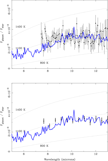
Figure 13: The contrast spectrum for HD 209458b plotted together with a model (Burrows et al. 2006) for the exoplanet emission. The planet emission is most consistent with models containing significant heat redistribution. The departure of the measurement from the model in the 8 $\mu$m region of the spectrum is significant and may place constraints on models of the planet emission. We have omitted wavelengths beyond 13 $\mu$m from the contrast spectrum because these data have lower SNR.

Spatial Axis Fit Parameters

AOR/nod	$A_{\theta}$	$\omega$	$\phi_{\theta}$	$x_{0}$	$m_{x}$	$A_{x}$	$\phi_{x}$
	[rad/time]	[cycles/nod]	[radians]	[pix]	[pix/nod]	[pix]	[radians]
AOR 7792/nod1	0.2699	2.9784	0.665	-5.2497	0.0042	0.0167	0.818
AOR 7792/nod2	”	2.9785	0.765	5.835	-0.0050	”	0.918
AOR 8048/nod1	”	2.9787	0.085	-3.871	-0.0295	”	0.238
AOR 8048/nod2	”	2.9785	0.135	6.25	-0.0104	”	0.288

Table 1: The parameters determined by fitting an elliptical pointing error to the source position along the spatial axis of the spectrometer slit. $A_{\theta}$ is the amplitude of the angular acceleration, $\omega$ is the angular frequency, $\phi_{\theta}$ is the angular phase, $x_{0}$ is the constant offset in the x position, $m_{x}$ is the linear change of position with time in the spatial axis, $A_{x}$ is the amplitude of the $x$ periodic function, and $\phi_{x}$, is the phase in the spatial axis.

Spectral Axis Fit Parameters

AOR/nod	$y_{0}$	$m_{y}$	$A_{y}$	$\phi_{y}$
	[pixels]	[pixels/nod]	[pixels]	[phase]
AOR 14817792/nod1	0.2149	-0.0242	0.0145	0.8474
AOR 14817792/nod2	0.3003	-0.0276	“	“
AOR 14818048/nod1	0.1175	-0.0202	“	“
AOR 14818048/nod2	0.2023	-0.0403	“	“

Table 2: The parameters for the telescope pointing model in the cross-slit (dispersion) axis: initial offset, $y_{0}$; linear drift, $m_{y}$; periodic amplitude, $A_{y}$; and phase, $\phi_{y}$. These values were determined by requiring self-similarity of the spectrum during the “star+planet” and “star only” intervals of the spectral time series.

Planet/Star Contrast Spectrum

wavelength ($\mu$)	contrast	error
7.67	0.0031	0.00025
8.15	0.0027	0.00019
8.63	0.0032	0.00020
9.12	0.0033	0.00022
9.60	0.0032	0.00022
10.09	0.0031	0.00021
10.57	0.0033	0.00023
11.05	0.0034	0.00026
11.54	0.0030	0.00028
12.02	0.0033	0.00029
12.51	0.0032	0.00029
12.99	0.0033	0.00033
13.47	0.0025	0.00040
13.96	0.0029	0.00046
14.44	0.0040	0.00049

Table 3: Data and 1-$\sigma$ error for the contrast spectrum of HD 209458b shown in the lower panel of Fig. 13.

References

- Bayard & Burgarolas (2004) Bayard, D. S., & Brugarolas, P. B. 2004, IOM, 3457-04-002.
- Beichman et al. (2006) Beichman, C., et al. 2006, ApJ, 639, 1166.
- Bouwman et al. (2006) Bouwman, J., Lawson, W. A., Dominik, C., Feigelson, E. D., Henning, T., Tielens, A. G. G. M., & Waters, L. B. F. M. 2006, ApJ, 653, L57.
- Bryden et al. (2006) Bryden, G., et al. 2006, ApJ, 636, 1098.
- Burrows et al. (2006) Burrows, A., Sudarsky, D., & Hubeny, I. 2006, ApJ, 650, 1140.
- Burrows (2007) Burrows, A. 2007, priviate communication.
- Carey (2007) Carey, 2007, priviate communication.
- Charbonneau, et al. (2000) Charbonneau, D., Brown, T. M., Latham, D. W., & Mayor, M. 2000, ApJ, 529, L45.
- Charbonneau, et al. (2002) Charbonneau, D., Brown, T. M., Noyes, R. W., & Gilliland, R. L. 2002, ApJ, 568, 377.
- Charbonneau et al. (2005) Charbonneau, D., et al. 2005 ApJ626, 523.
- Deming et al. (2005a) Deming, D., Seager, S., Richardson, L. J., & Harrington, J. 2005a, Nature, 434, 740.
- Deming et al. (2005b) Deming, D., Brown, T. M., Charbonneau, D., Harrington, J., & Richardson, J. L. 2005b, ApJ, 622, 1149.
- Deming et al. (2006) Deming, D., Harrington, J., Seager, S., Richardson, L. J. 2006, ApJ, 644, 560.
- Fortney et al. (2006) Fortney, J. J., Cooper, C. S., Showman, A. P., Marley, M. S., & Freedman, R. S. 2006, ApJ, 652, 746.
- Grillmair et al. (2007) Grillmair, C. J, Charbonneau, D., Burrows, A., Armus, L, Stauffer, J., Meadows, V., Van Cleve, J., & Levine, D. 2007, ApJ, 658L, 115.
- Harrington et al. (2006) Harrington, J., Hansen, B. M., Luszca, S. H., Seager, S., Deming, D., Menou, K., Cho, J., & Richardson, J. L. 2006, Science, 314, 623.
- Higdon et al. (2004) Higdon, S. J. U. et al. 2004, PASP, 116, 975.
- Houck et al. (2004) Houck, J. R. 2004, ApJS, 154, 18.
- Kurucz (1992) Kurucz, R. L. 1992, IAU Symp. 149, Stellar Populations in Galaxies, 225.
- Knutson et al. (2007) Knutson, H. A., Charbonneau, D., Noyes, R. W, Brown, T. M., & Gilliland, R. L. 2007, ApJ, 655, 564.
- Morales-Calderón et al. (2006) Morales-Calderón et al. 2006, ApJ, 653, 1454.
- Nagano & Matsuyama (1979) Nagano, M. & Matsuyama, T. 1979, Computer Graphics and Image Processing, 9, 394.
- Richardson et al. (2003) Richardson, L. J., Deming, D., Wiedemann, G., Goukenleuqe, C., Steyert, D., Harrington, J., & Esposito, L. W. 2003, ApJ, 584, 1053.
- Richardson et al. (2007) Richardson, J. L., Deming, D., Horning, K., Seager, S., & Harrington, J. 2007, Nature, 445, 892.
- Werner et al. (2004) Werner, M. W., et al. 2004, ApJS, 154, 1.