Exciting Dark Matter and the INTEGRAL/SPI 511 keV signal

Abstract

We propose a WIMP candidate with an “excited state” 1-2 MeV above the ground state, which may be collisionally excited and de-excites by $e^{+}e^{-}$ pair emission. By converting its kinetic energy into pairs, such a particle could produce a substantial fraction of the 511 keV line observed by INTEGRAL/SPI in the inner Milky Way. Only a small fraction of the WIMPs have sufficient energy to excite, and that fraction drops sharply with galactocentric radius, naturally yielding a radial cutoff, as observed. Even if the scattering probability in the inner kpc is $\ll 1\%$ per Hubble time, enough power is available to produce the $\sim 3\times 10^{42}$ pairs per second observed in the Galactic bulge. We specify the parameters of a pseudo-Dirac fermion designed to explain the positron signal, and find that it annihilates chiefly to $e^{+}e^{-}$ and freezes out with the correct relic density. We discuss possible observational consequences of this model.

I Introduction

One of the central unsolved problems of both particle physics and cosmology is the nature of the dark matter. Although well motivated candidates exist, for instance a weakly-interacting massive particle (WIMP) or axion, they have thus far eluded definitive detection. This makes indirect signals, such as anomalous particle production in the Galaxy, especially interesting as a possible indicator of the physics of dark matter.

I.1 The Positron Annihilation Signal

In 1970, the first detection of a gamma-ray line in the Galactic center found a line center at $473\pm 30{\rm keV}$, causing the authors to doubt its true origin Johnson et al. (1972). Leventhal Leventhal (1973) soon pointed out that the spectrum was consistent with positronium emission, because positronium continuum could confuse the line fit in a low-resolution spectrograph, but worried that the implied annihilation of $7\times 10^{42}$ pairs/s was several orders of magnitude larger than his estimate of the pair creation rate from cosmic ray interactions with the interstellar medium (ISM). Since then, other balloon and space missions such as SMMShare et al. (1988), CGRO/OSSE Kinzer et al. (2001) and most recently the SPI spectrograph Attié et al. (2003); Vedrenne et al. (2003) aboard the International Gamma-Ray Astrophysics Laboratory (INTEGRAL) have greatly refined these measurements Knödlseder et al. (2003); Weidenspointner et al. (2006) (see Teegarden et al. (2005) for a summary of previous measurements). We now know that the line center is $510.954\pm 0.075{\rm keV}$, consistent with the unshifted $e^{+}e^{-}$ annihilation line Churazov et al. (2005) but still find the estimated annihilation rate of $\sim 3\times 10^{42}$ $e^{+}e^{-}$ pairs per second Knödlseder et al. (2003); Weidenspointner et al. (2006) surprising. The origin of these positrons remains a mystery.

The OSSE data showed a bulge and a disk component, with $\sim 25\%$ of the flux in the diskKinzer et al. (2001). The most recent INTEGRAL data show mainly the bulge component, approximated by a Gaussian with FWHM $6^{\circ}$ Weidenspointner et al. (2007). The data are consistent with a disk component several times fainter than the bulge, when Galactic CO maps are used as a disk template. The spatial distribution of the ortho-Ps (positronium) 3-photon continuum and 511 keV line are mutually consistent, with $92\pm 9\%$ of the pairs annihilating through Ps Weidenspointner et al. (2006). The faintness of the disk component constrains the expected (conventional) $e^{+}$ production modes: cascades from cosmic ray interaction with the ISM, and nucleosynthetic processes during supernovae both would have a disk component. In order to achieve the observed bulge/disk ratio with type Ia SNe, one must assume that the positrons from the disk migrate to the bulge before they annihilate; otherwise the bulge signal would only be $\sim 10\%$ of that observed Prantzos (2006).

Indeed, Kalemci et al.Kalemci et al. (2006) find that the quantity of pairs alone rules out SNe as the only source. Using SPI observations of SN 1006 (thought to be type Ia), they derive a $3\sigma$ upper limit of 7.5% for the positron escape fraction. An escape fraction of 12% would be required to produce all of the positrons in the Galaxy, but even then they would be distributed throughout the disk, like the 1.8 MeV line from ²⁶Al Plüschke et al. (2002), rather than concentrated in the Galactic center. Hypernovae remain a possibility, if there are more than 0.02 SN 2003dh-like events (SNe type Ic) per century Cassé et al. (2004). GRB rates of one per $8\times 10^{4}$ yr $\times(E_{GRB}/10^{51}{\rm erg})$ are also sufficient Parizot et al. (2005).

It is estimated that microquasars could contribute enough positrons to produce approximately 1/3 of the annihilation signal Guessoum et al. (2006), but again, it is not clear that their spatial distribution is so strongly biased towards the Galactic bulge.

In summary, no obvious astrophysical explanation for this positron production exists; proposals in the literature have difficulty explaining the size or spatial distribution of the signal, and often both. While it is still possible that conventional (or more exotic) astrophysical sources could produce the entire signal, the concentration of dark matter in the Galactic center motivates consideration of an alternative hypothesis: that some property of dark matter is responsible for the signal.

I.2 Dark Matter

In recent years, WIMP annihilation scenarios have been invoked to explain a number of high energy astrophysical phenomena (see Bertone et al. (2005) for a review). It is possible to create the pairs directly from WIMP annihilation if the WIMP mass is a few MeV Boehm et al. (2004), but this mass range has no theoretical motivation. In extensions to the Standard Model which addresses the hierarchy problem, such as supersymmetry, the WIMP mass is usually above the weak scale (100 GeV - 1 TeV) and the annihilation products come out at energies very large compared to $m_{e}$. In the absence of a dense environment where a cascade can develop (column densities of $\sim 10^{27}{\rm~{}cm}^{-2}$ are required for the $\gamma\rightarrow e^{+}e^{-}$ step), there is no way to partition the energy of these particles into the many thousands of pairs required for each WIMP annihilation. Consequently, it has generally been concluded that weak scale dark matter has nothing to do with the observed positronium annihilation signal. However, we shall see that WIMPs in this mass range could still play a role: they could convert WIMP kinetic energy into pairs via scattering.

The kinetic energy of a 500 GeV WIMP moving at 500 km/s is $>511$ keV. If the WIMP has something analogous to an excited state – for whatever reason – inelastic scattering could occur, raising one or both of the WIMPs to this excited state. If the energy splitting is more than $2m_{e}$, the decay back to ground state would likely be accompanied by the emission of an $e^{+}e^{-}$ pair. One tantalizing feature of this mechanism is that it provides access to the vast reservoir of kinetic energy in the WIMPs (roughly $10^{60}$ erg for the Milky Way), such that bleeding off $3\times 10^{42}~{}{\rm MeV}/\rm{s}=5\times 10^{36}$ erg/s reduces the kinetic energy by a negligible amount, even over the age of the Universe. Indeed, the unexplained excess in the bulge is much smaller than that. Therefore, this scattering would have negligible kinematic effect on the dark matter halo, except perhaps in its innermost parts.

In this paper, we propose that the positrons in the center of the Galaxy arise precisely from this process of “exciting” dark matter (XDM). Remarkably, such a phenomenon is quite natural from the perspective of particle physics in theories with approximate symmetries in the dark sector, which are generally accompanied by nearly degenerate states, which can serve as excited states. Although the MSSM dark matter candidate, the neutralino, does not exhibit such a property, this is simply the result of the restricted field content of the MSSM, with no additional approximate symmetries present. Other WIMPs, both arising in supersymmetry and from strong dynamics easily give this phenomenology – and usually without upsetting the desirable properties of WIMP models.

The layout of this paper is as follows: in section II we discuss the basic properties of such a scenario, and constraints on the model from the annihilation signal. In section III, we review a simple example from particle physics with the required properties, utilizing a single pseudo-Dirac fermion as dark matter. In this scenario we will also comment on the annihilation rate into standard model particles and other direct and indirect tests of the model.

II Constraints from the 511 keV signal

While the spectral line and continuum data from SPI are robust when averaged over the entire inner Galaxy, the spectrum in each spatial pixel is noisy. In order to stabilize the fit and robustly determine the total positronium (Ps) annihilation rate in the bulge, the SPI maps are cross-correlated with spatial templates. Because the Ps emission in the inner Galaxy does not follow the stellar mass distribution, the choice of templates is somewhat arbitrary. Representing the disk with a CO map, and the bulge with a Gaussian, Weidenspointner et al. Weidenspointner et al. (2006) obtain continuum Ps fluxes in their “analysis bands” of $f_{b}=0.86^{+0.15}_{-0.13}\times 10^{-3}{\rm~{}ph~{}cm^{-2}~{}s^{-1}}$ and $f_{CO}=1.92^{+0.49}_{-0.48}\times 10^{-3}{\rm~{}ph~{}cm^{-2}~{}s^{-1}}$ for the bulge and disk, respectively, finding 31% of the emission is in the bulge. Because the bulge component covers less solid angle than the disk, its surface brightness is much higher. Using the full SPI response matrix they then obtain a total Ps continuum (bulge plus disk) of $(3.11\pm 0.56)\times 10^{-3}{\rm~{}ph~{}cm^{-2}~{}s^{-1}}$ and line flux of $(9.35\pm 0.54)\times 10^{-4}{\rm~{}ph~{}cm^{-2}~{}s^{-1}}$. For a Galactocentric distance of 8 kpc = $2.4\times 10^{22}{\rm~{}cm}$, this implies a total pair annihilation rate of $1.1\times 10^{43}{\rm~{}s}^{-1}$, or $3.4\times 10^{42}{\rm~{}s}^{-1}$ for the bulge. Because of order 10% of that is explained by SNe Prantzos (2006), we take $3\times 10^{42}{\rm~{}s}^{-1}$ as the excess pair creation rate in the Galactic bulge to be explained.

SPI also measures the width of the annihilation line to be $2.37\pm 0.25~{}{\rm keV}$ FWHM, which is consistent with a warm ($7000<T_{e}<4\times 10^{4}{\rm~{}K}$) weakly ionized medium Churazov et al. (2005). Knowledge of the state of the ISM in the inner Galaxy may be used to constrain the injection energy of the $e^{+}$ to less than a few MeV Jean et al. (2006), which agrees with the constraints set by Beacom et al. using internal bremsstrahlung Beacom et al. (2005) and propagation Beacom and Yuksel (2006). In our model, the few MeV constraint applies to the splitting between the states, not the mass of the WIMPs themselves.

II.1 Form of the cross section

In this section we use elementary considerations of the phase-space density and expected $v$-dependence of the cross section to derive constraints on the ratio of the splitting to the mass $(\delta/M)$ from the slope of the 511 keV emission.

The velocity-averaged rate coefficient (i.e. number of scatterings per time per density) $\langle\sigma v\rangle$ is

$$\langle\sigma v\rangle(\mathbf{r})=\int d^{3}vd^{3}v^{\prime}f(\mathbf{v,r})f(\mathbf{v^{\prime},r})\sigma(v_{rel})v_{rel}$$ (1)

where $f(\mathbf{v,r})$ is the phase-space density of particles at position $\mathbf{r}$ and velocity $\mathbf{v}$, $\sigma(v_{rel})$ is the inelastic scattering cross section as a function of the velocity difference $v_{rel}=|\mathbf{v}-\mathbf{v^{\prime}}|$, which vanishes below threshold ($v_{rel}<v_{thresh}$), and the integrals are taken over all velocities.

In order to make an estimate of the parameters involved, we approximate the velocity distribution as isotropic with no particle-particle velocity correlations (caused by e.g. net rotation of the DM halo). This reduces $\langle\sigma v\rangle$ and $f$ to functions of scalar $r$ and $v$. The cross section of the proposed pseudo-Dirac fermion has a weak dependence on velocity, so we first focus on a simplified form of $\langle\sigma v\rangle$ where the velocity dependence is entirely encoded in the phase space of the final state particles, i.e., where the form of the cross section is

$$\sigma v_{rel}=\begin{cases}\sigma_{mr}\sqrt{v_{rel}^{2}-4\delta/M_{\chi}}&v_{rel}^{2}>4\delta/M_{\chi}\\ 0&v_{rel}^{2}\leq 4\delta/M_{\chi}\end{cases}$$ (2)

Here $\sigma_{mr}$ is independent of velocity and is the approximate cross section in the moderately relativistic limit (where the second factor goes to $v$). Here $\delta$ is the splitting of the excited state from the ground state and $M_{\chi}$ is the mass of the wimp. The threshold velocity for excitation is $v_{thresh}=\sqrt{4\delta/M_{\chi}}$, so the integral becomes

$$\langle\sigma v\rangle(r) =8\pi^{2}\sigma_{mr}\int_{0}^{\infty}v^{2}f(v,r)dv\int_{0}^{\infty}v^{\prime 2}f(v^{\prime},r)dv^{\prime}$$ (3)

$$\times\int_{-1}^{1}d(\cos\theta)\sqrt{v_{rel}^{2}-v_{thresh}^{2}}$$

with

$$v_{rel}^{2}=v^{2}+v^{\prime 2}+2vv^{\prime}\cos\theta$$ (4)

This conveniently separates the problem into a question of particle physics ($\sigma_{mr}$) and a question of astrophysics (the phase-space densities).

II.2 DM velocity distribution

The WIMP velocity distribution depends on the details of the formation history of the Galaxy, but for simplicity we use a Boltzmann approximation. Although there may be some WIMPs in the inner Galaxy moving faster than escape velocity, it is reasonable to assume that the distribution goes to zero rapidly for $v>v_{esc}(r)$. Therefore, we adopt

$$f(v,r)=\begin{cases}N\exp(-v^{2}/2v_{rms}^{2})&v\leq v_{esc}\\ 0&v>v_{esc}\end{cases}$$ (5)

with 1-D velocity dispersion $v_{rms}=200{\rm~{}km/s}$. $N$ normalizes this so that $\int^{v_{esc}}d^{3}vf(v,r)=1$. Following Merritt et al. Merritt et al. (2005) we use a DM halo profile of the form

$$\rho=\rho_{0}\exp\left[-\frac{2}{\alpha}\left(\frac{r^{\alpha}-R_{\odot}^{\alpha}}{r_{-2}^{\alpha}}\right)\right]$$ (6)

where $\rho_{0}=0.1-0.7~{}{\rm GeV}$ Yao et al. (2006) is the DM density at the Solar circle ($r=R_{\odot}$), $r_{-2}=25{\rm~{}kpc}$ is the radius at which the logarithmic slope of the profile is -2, and $\alpha\approx 0.2$ is a parameter of the profile. This profile is inspired by a fitting formula for the logarithmic slope of densityNavarro et al. (2004):

$$\frac{d\ln\rho}{d\ln r}=-2(r/r_{-2})^{\alpha}$$ (7)

and agrees well with simulations Merritt et al. (2005).

This profile only contains the dark matter, which does not dominate in the inner parts of the Galaxy. To estimate the escape velocity of the Milky Way, we note that the rotation curve is nearly flat with a circular velocity $v_{c}\approx 220{\rm~{}km/s}$ out to far beyond the solar circle Fich et al. (1989). In the Merritt profile the scale radius of $r_{-2}$ contains much of the mass of the Galaxy, so we make the (conservative) approximation that the rotation curve is flat to $20{\rm~{}kpc}$ and then there is no mass beyond that radius. A flat rotation curve implies that enclosed mass $M(r)=rv_{c}^{2}/G$, so $\rho(r)\sim r^{-2}$. This density profile differs from the Merritt profile because it includes baryonic matter, which dominates the mass density in the inner part of the Milky Way. (The Black Hole dominates only inside the inner 1 pc, so we neglect its influence.)

The value of the one-dimensional velocity dispersion is chosen to agree with simulations Governato et al. (2007). Although some authors have correctly pointed out that in DM-only halos the dispersion decreases in the center (e.g. Ascasibar et al. (2006)), simulations including gas physics and star formation indicate an increase Governato et al. (2007). We defer a detailed discussion of these and related issues to a future paper.

The gravitational potential $\Phi=-v_{c}^{2}$ at $r=r_{-2}$, so

$$\Phi(r)=-v_{c}^{2}-\int_{r}^{r_{-2}}\frac{GM(r^{\prime})}{r^{\prime 2}}dr^{\prime}=v_{c}^{2}[\ln(r/r_{-2})-1]$$ (8)

therefore,

$$v_{esc}(r)=\sqrt{-2\Phi(r)}=\begin{cases}v_{c}\sqrt{2[1-\ln(r/r_{-2})]}&\text{for~{}}r<r_{-2}\\ v_{c}\sqrt{2r_{-2}/r}&\text{for~{}}r>r_{-2}\end{cases}$$ (9)

which for $v_{c}=220{\rm~{}km/s}$ gives $v_{esc}(8{\rm~{}kpc})=431{\rm~{}km/s}$ and $v_{esc}(0.5{\rm~{}kpc})=674{\rm~{}km/s}$. Thus an energy threshold for the inelastic scattering corresponding to about $v_{rel}=1000{\rm~{}km/s}$ will cause a sharp cutoff beyond a Galactocentric radius of 400 pc (about $3^{\circ}$) as observed by INTEGRAL. Other assumptions may be made about the mass profile outside of $20{\rm~{}kpc}$, but since any additional velocities add in quadrature, they do not modify this result greatly.

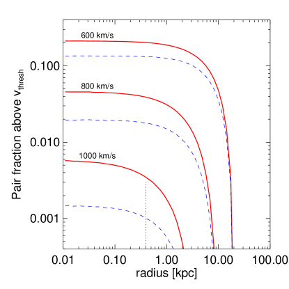
Figure 1: The fraction of pairs with velocity above $v_{thresh}$ of 600, 800, or 1000 km/s, for $v_{rms}=200{\rm~{}km/s}$ (solid) and $v_{rms}=180{\rm~{}km/s}$ (dashed). The approximate half-max radius of the observed 511 keV emission (vertical dotted) is shown for reference.

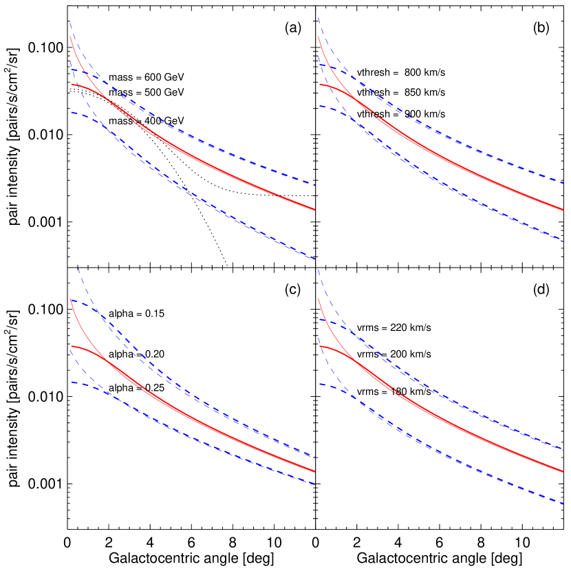
Figure 2: Model curves for the constant sigma model in Eq (2), taking $\sigma_{mr}=1.3\times 10^{-26}{\rm~{}cm}^{2}\left(\frac{0.3~{}{\rm GeV}/cm^{3}}{\rho_{0}}\right)^{2}=2.4\times 10^{-27}-1.2\times 10^{-25}{\rm~{}cm}^{2}$, both unsmoothed (thin) and smoothed by a $3^{\circ}$ FWHM beam (thick) to approximate the spatial response of SPI. In all cases the solid red lines represent our fiducial model ($M=500~{}{\rm GeV}$, $v_{thresh}=850{\rm~{}km/s}$, and halo parameters $v_{rms}=200{\rm~{}km/s}$, and Merritt index $\alpha=0.2$), and dashed blue lines represent variations of one parameter. (a) $M=400,500,600~{}{\rm GeV}$ with $\delta$ held fixed at $1~{}{\rm MeV}$ so that $v_{thresh}=950,850,776{\rm~{}km/s}$, respectively. (b) $v_{thresh}=800,850,900{\rm~{}km/s}$, keeping $M=500~{}{\rm GeV}$ while $\delta$ now varies above and below $1~{}{\rm MeV}$. (c) The Merritt profile index $\alpha$ is varied (see Eq 6). (d) The RMS velocity in the inner Milky Way is varied. This is assumed to be constant with radius. The observed $6^{\circ}$ FWHM signal (lower dotted line) and that signal plus an arbitrary baseline of 0.002 (upper dotted line) are shown in (a). The SPI zero is set by measurements $10^{\circ}$ off the Galactic plane to correct for instrumental background.

Figure 3: Same as Fig. 2, but using the full expression for the inelastic scattering cross section (Eq. 19) derived in Appendix A, setting the coupling $\lambda_{+}=\lambda_{-}=0.18$ and $\rho=0.4~{}{\rm GeV}/{\rm cm}^{3}$.

It is instructive to consider the fraction of WIMP pairs with a relative velocity above threshold, as a function of radius. This provides a sense of how many pairs are participating in the inelastic scattering, independent of the detail of the particle physics model. This pair fraction is shown in Fig. 1 for three values of $v_{thresh}$ and two values of $v_{rms}$, the 1-D velocity dispersion.

II.3 Comparison with Observations

To compare this model to the 511 keV map, we next integrate along the line of sight

$$\int_{0}^{\infty}dl\langle\sigma v\rangle(r)n^{2}(r)$$ (10)

to obtain the number of pair creations per area per time. Figs. 2, 3 show the line of sight integral for various particle model and halo profile parameters. For comparison, the most recent analysis of the INTEGRAL SPI signal finds a $6^{\circ}$ FWHM Gaussian Weidenspointner et al. (2007) in agreement with previous measurements by OSSE Kinzer et al. (2001). This corresponds to a pair intensity (inferred from both line and Ps continuum) of

$$I_{\rm pair}=\frac{L_{\rm pair}}{4\pi R_{\odot}^{2}}\frac{\exp(-\theta^{2}/2a^{2})}{2\pi a^{2}}$$ (11)

where $L_{\rm pair}=3\times 10^{42}$ pairs/s, $a=0.044$ rad (i.e., $6^{\circ}/2.355$), $R_{\odot}=8{\rm~{}kpc}$, and $\theta$ is the Galactocentric angle. This function peaks at $I\approx 0.03$ pairs${\rm~{}s}^{-1}{\rm~{}cm}^{-2}{\rm~{}sr}^{-1}$, and is shown in Figs. 2,3 for comparison. In these plots, we have attempted to employ standard values from $\alpha,\rho_{0}$, and $v_{rms}$ for the fiducial model. However, by taking more optimal values for all parameters, a cross section of $\sigma_{mr}\simeq 3\times 10^{-28}{\rm~{}cm}^{2}$ would be sufficient to generate an acceptable rate to satisfy the INTEGRAL measurement.

None of the model lines in Fig. 3 are in perfect agreement with the Gaussian, but keep in mind:

• The Gaussian form chosen by the SPI team is only an approximation. A more thorough analysis would fit the SPI data directly to a class of XDM models and compare likelihoods, as in Ascasibar et al. (2006).

• The substantial instrumental backgrounds in SPI are removed by subtracting observations of “blank” sky $10^{\circ}$ off the Galactic plane. We adjust the zero-point of the INTEGRAL measurements to match the model at $10^{\circ}$, improving the agreement (see upper dotted line, Figs. 2 and 3).

• We have chosen a narrow class of DM halo profiles for this benchmark model. A different profile could improve agreement with the Gaussian.

• Significant variation of the velocity dependence of the cross section could arise in different particle physics models

• Other factors could alter the results, e.g. the elastic scattering of WIMPs (see appendix) at some level may alter the entropy in the inner part of the halo and cause significant departures from the assumed velocity and radial distributions.

Whatever deficiencies our model may suffer from in terms of the spatial distribution of the positrons, they are less severe than annihilation models (e.g. Boehm et al. (2004)) because XDM provides a mechanism for a radial cutoff. Regardless of the details of $f(r,v)$ this is an appealing aspect of XDM.

The question remains whether such a model of dark matter could naturally arise from particle physics considerations. In the following section, we will see that such models occur simply in extensions of the standard model.

III Models of Exciting Dark Matter

It is quite straightforward to find models of this sort. A model of composite dark matter, for instance, involving a bound state of constituent particles, would be expected to have precisely this sort of structure, arising from its excited states . However, one needn’t invoke complicated dynamics in order to generate a splitting, as an approximate symmetry will suffice.

An example of this is the neutron-proton mass difference, which is protected by an approximate isospin symmetry. Consequently, although the overall mass scale for the nucleons is GeV, the splitting is small, and protected against radiative corrections by the symmetry. We will take a similar approach here.

Let us consider a Dirac fermion, composed of two Weyl fermions $\chi_{1,2}$. We will require the presence of a scalar field $\phi$, which will be light, and mediate the process of excitation. The Lagrangian we consider is

$${\cal L} = \frac{1}{2}\partial_{\mu}\phi\partial^{\mu}\phi+\chi_{i}^{\dagger}\sigma_{\mu}\partial^{\mu}\chi_{i}-m_{D}\chi_{1}\chi_{2}$$

$$-\lambda_{1}\phi\chi_{1}\chi_{1}-\lambda_{2}\phi\chi_{2}\chi_{2}-V(\phi).$$

This can be justified with a ${\bf Z}_{4}$ symmetry, under which $\chi_{1,2}\rightarrow e^{\pm i\pi/2}\chi_{1,2}$ and $\phi\rightarrow-\phi$.

It is easiest to work in the basis $\chi,\chi_{*}=1/\sqrt{2}(\chi_{1}\mp\chi_{2})$. In this basis the mass matrix for the $\chi$’s is

$$M=\begin{pmatrix}\lambda_{+}\phi-m_{D}&\lambda_{-}\phi\cr\lambda_{-}\phi&\lambda_{+}\phi+m_{D}\end{pmatrix},$$ (13)

where $\lambda_{\pm}=\frac{1}{2}(\lambda_{1}\pm\lambda_{2})$. There are simple conclusions to draw from this expression. At leading order, the Dirac fermion is understood as two degenerate Majorana fermions. If the ${\bf Z}_{4}$ symmetry is broken weakly to ${\bf Z}_{2}$, for instance by a $\phi$ expectation value, we expect these states to be split by a small amount $\delta=2\lambda_{+}\left\langle{\phi}\right\rangle$. It should be noted that because this is a symmetry breaking parameter, it can be naturally much smaller than the mass of the dark matter particle. We shall consider a simple origin for the vev shortly, but for now will take it as a free parameter.

a)
b)

Figure 4: Excitation diagrams for $\chi\chi\rightarrow\chi^{*}\chi$.

The process of excitation is mediated by the Feynman diagram of Fig.4a. At very low velocity, one needs to sum the ladder diagrams . The calculation of the cross section is given in the appendix. Qualitatively, however, the cross section is often approximately geometric, i.e., set by the scale of the characteristic momentum transfer. That is, $\sigma v\sim v/q^{2}\sim v/m\delta\sim 10^{-19}{\rm~{}cm}^{3}/\rm{s}$. This large excitation cross section, interestingly, does not occur for large coupling, but rather when the perturbative expansion in $\lambda^{2}/4\pi^{2}v$ breaks down.

The origin of the splitting will come from an expectation value of $\phi$. This can be derived from a potential of the form

$$V(\phi)=-\frac{m_{\phi}^{2}}{2}\phi^{2}+\frac{\kappa}{4}\phi^{4}$$ (14)

from which we yield a vacuum expectation value (vev) $\left\langle{\phi^{2}}\right\rangle=m_{\phi}^{2}/\kappa$. The mass splitting is then just $\delta=2\lambda_{+}m_{\phi}/\sqrt{\kappa}$.

The presence of such a vev seems to imply the existence of domain walls, which would be at the limit of what is allowed with regard to dominating the energy density of the universe Kolb and Turner (1990). This can be cured by the presence of cubic term $a\phi^{3}$, or the promotion of the symmetry to a (continuous) gauge symmetry. Although the cubic term is aesthetically unappealing, as our focus here is on the phenomenology of such a model with regard to present astrophysics, we shall accept such a term and defer more appealing solutions to future work.

At this point we have only explained the process of excitation, but have not included the production of $e^{+}e^{-}$ pairs. This arises quite simply from a mixing term of the form

$$\alpha\phi^{2}hh^{*}.$$ (15)

Such a term induces a mixing $\theta_{mix}\sim\alpha\left\langle{\phi}\right\rangle/m_{h}$. Thus, decays of the excited state into the lighter state proceed through the diagram in Fig. 5.

Figure 5: Decay of the excited state into the ground state.

III.1 XDM in the early universe

While some worries, such as domain walls, can be cured simply, there are a number of non-trivial issues that must be addressed, most notably, the questions related to Big Bang Nucleosynthesis (BBN) and the relic abundance of the XDM.

Let us begin by addressing the lifetimes of the various particles. Both excited and unexcited states of the dark matter will come into thermal equilibrium in the early universe, with the excited state decaying into the lighter state with an approximate lifetime

$$\tau_{\chi^{*}}^{-1}\sim\frac{\lambda_{-}^{2}\sin^{2}\theta_{mix}y_{e}^{2}\delta^{5}}{\mu^{4}}$$ (16)

while the scalar $\phi$ decays with lifetime

$$\tau_{\phi}^{-1}\approx\frac{m_{\phi}}{8\pi}y_{x}^{2}\sin^{2}\theta_{mix},$$ (17)

where $y_{x}$ is the Yukawa coupling of the heaviest fermion into which $\phi$ can decay. (In general, as $m_{\phi}\mathop{}_{\textstyle\sim}^{\textstyle<}1{\rm GeV}$, this is $y_{\mu}$ or $y_{e}$.) With reasonable values for the mixing parameter, a scalar with mass $m\mathop{}_{\textstyle\sim}^{\textstyle>}1{\rm MeV}$ will decay before nucleosynthesis. However, the decay of the excited state into the lighter state will naturally occur after nucleosynthesis, but well before recombination. Because of the low baryon to photon ratio, these positrons should thermalize before affecting the light element abundances, but it would be interesting to consider whether any effects would be observable.

Although structurally somewhat different, the relic abundance calculation for XDM is ultimately very similar to that of standard WIMPs. It is simplest, conceptually, if one separates the sectors of the theory into a dark sector ($\chi,\chi^{*},\phi$) and the standard model sector. The relevant direct coupling between the two sectors is $\alpha$. Naturalness tells us that $\alpha\mathop{}_{\textstyle\sim}^{\textstyle<}m_{\phi}^{2}/v_{higgs}^{2}\mathop{}_{\textstyle\sim}^{\textstyle<}10^{-4}$, so as not to significantly correct the $\phi$ vev.

The relic abundance proceeds in a slight variation of usual WIMP freezeout. Here, $\chi$ will stay in equilibrium with $\phi$, which, in turn, stays in thermal equilibrium with the standard model. Direct scatterings $\phi\phi\leftrightarrow hh$ are in equilibrium at temperatures above the Higgs mass for $\alpha\mathop{}_{\textstyle\sim}^{\textstyle>}10^{-8}$, thus we can reasonably tolerate $m_{\phi}\mathop{}_{\textstyle\sim}^{\textstyle>}10{\rm MeV}$ from the naturalness constraint. In this way, the temperature of the dark sector is made equal to the temperature of the standard model particles. Whether this persists below the Higgs mass depends on $\alpha$. The s-channel annihilation into standard model fermions shown in Fig. 6a has a relativistic cross section $\sigma_{ann}=\alpha^{2}m_{f}^{2}/(8\pi m_{h}^{4})$. This should keep annihilations in thermal equilibrium down to $T=m_{\mu},m_{c}\sim m_{\tau},m_{b}$ for $\alpha\mathop{}_{\textstyle\sim}^{\textstyle>}10^{-4},10^{-6},10^{-7}$, respectively.

The annihilation rate of $\chi$ into $\phi$ occurs through the diagram in Fig 6b, with a cross section for $\chi\chi\rightarrow\phi\phi$ annihilation of $\sigma_{ann}v_{rel}=8\lambda^{4}/(\pi M_{\chi}^{2})$. The relic abundance from the freezeout of such an interaction is Kolb and Turner (1990) (assuming equilibrium with the standard model) $\Omega h^{2}\approx 2\times 10^{-11}{\rm GeV^{-2}}/\left\langle{\sigma_{ann}v_{rel}}\right\rangle$, which yields an acceptable relic abundance for $\lambda\sim\sqrt{M/100{\rm TeV}}$, or, roughly $\lambda\sim 1/10$, which is precisely the region in which the excitation process is maximal. This result should not be surprising - it is the usual result that a weak scale particle with perturbative coupling freezes out with the appropriate relic density. A rigorous study of the allowed parameter range is clearly warranted.

a)                   b)

Figure 6: Diagrams contributing to thermal equilibrium in the dark sector and between the dark sector and the visible sector.

III.2 Other decays and signals

Although the freezeout process of XDM is similar to that of an ordinary WIMP, the scattering and annihilation products can clearly be different. One important feature is that the annihilation products are typically electrons and neutrinos for $m_{\phi}<2m_{\pi}$. However, unlike, e.g., MeV dark matter, when the particles annihilate the resulting electrons and positrons are extremely energetic. This is intriguing because both the HEAT data Coutu et al. (1999) and the “haze” from the center of the galaxy Finkbeiner (2004a, b) point to new sources of multi-GeV electrons and positrons. Here, these high energy particles (from boosted on-shell $\phi$ particles) are related to the low energy positrons detected by INTEGRAL (from off-shell $\phi$ particles). Such high energy particles may create high-energy gamma rays from inverse scattering off starlight which could be observed in the future GLAST mission. We leave detailed analysis of these possibilities for future work.

It should be noted that the electron and positron can be closed to allow a decay to two photons. Such a process is considerably suppressed, however, being down by a loop factor and suppressed by $\alpha$. Consequently, these monochromatic photons should be produced at a rate roughly $10^{-5}$ that of the positron production rate, and are unlikely to be detectable within the diffuse background (see, e.g., the discussion in Beacom and Yuksel (2006)).

IV Discussion - other observable consequences

IV.1 Cluster heating

In the most massive galaxy clusters, the velocity dispersion is high (up to $\sim 1000{\rm~{}km/s}$ 1-D), and the majority of pair velocities may be above threshold. It is doubtful that the $e^{+}e^{-}$ signal could be seen by the current generation of $\gamma-$ray telescopes, nor could the redshifted cosmological signal be seen yet. However, the kinetic energy of the pairs (which is assumed to be $\,\hbox to0.0pt{\raise 2.15277pt\hbox{$<$}\hss}{\lower 4.30554pt\hbox{$\sim$}}\,m_{e}$ when they are created) must heat the intergalactic plasma. In the intergalactic medium (IGM), losses due to synchrotron and inverse-Compton scattering are negligible at these energies. Losses are dominated by bremsstrahlung and perhaps Alfven wave excitation (see Loewenstein et al. (1991)), and both of these mechanisms heat the few $\times 10^{6}$K plasma in the IGM.

The powerful X-ray emission from bremsstrahlung in galaxy clusters (e.g. Perseus, Virgo) must either be balanced by significant heating (perhaps from AGN) or else cooling matter must fall into the cores. Such cooling flows have been sought for years, but never found at the level expected. Recent X-ray spectroscopy has shown much less emission at $\sim 1/3$ of the virial temperature than that expected from simple radiative cooling models Peterson and Fabian (2006). Alternatives, such as light DM annihilation Ascasibar (2007) have been suggested, but once again XDM can provide similar results. Especially noteworthy would be models of XDM with $\langle\sigma v\rangle$ rising as a higher power of $v$; these could produce a substantial fraction of the power needed to balance X-ray cooling in rich clusters. Furthermore, in such scenarios, the number of non-thermal (mildly relativistic) electrons could distort the SZ effect in small but detectable ways. Because estimates of cluster heating and SZ signal are strongly model-dependent, we defer discussion of this to a future paper.

IV.2 BH accretion

The $z\sim 6$ quasars discovered by the SDSS Fan et al. (2003) can be produced in simulations (Yuexing Li, priv. comm.) but only by seeding the simulations with $200M_{\odot}$ black holes at $z\sim 30$. A mechanism of dissipative scattering, such as XDM, provides the possibility of super-Eddington accretion. This could be important at high $z$, before baryons have had a chance to cool into potential wells, perhaps seeding the universe with black holes at early times. At later times, however, the more efficient cooling of baryons makes it unlikely that XDM accretion is a significant factor in BH growth in general.

V Conclusions

We propose that dark matter is composed of WIMPs which can be collisionally excited (XDM) and de-excite by $e^{+}e^{-}$ pair emission, and that this mechanism is responsible for the majority of the positronium annihilation signal observed in the inner Milky Way. A simple model of a pseudo-Dirac fermion with this property is presented, though other models with similar phenomenology are likely possible. The XDM framework is strongly motivated by a specific problem, but has a rich set of implications for cluster heating, BH formation, and other phenomena. The model naturally freezes out with approximately the right thermal relic density, and annihilations today go mainly to $e^{+}e^{-}$. Although XDM is dissipative, it does not jeopardize stability of observed structure or disagree with any other current observations.

Appendix A Excitation Cross Section

The process of excitation arises from a sum of all ladder diagrams in addition to the tree level diagrams. We sum these using the spectator approach, where we take the intermediate fermion lines to be on-shell. Neglecting logarithmic dependencies on the momenta and scalar mass, one then finds the n^th diagram to be proportional to $q^{-2}(\lambda^{2}/v)^{n}$, where $\lambda^{2}=\lambda_{-,+}^{2},\lambda_{-}\lambda_{+}$ depending on the diagram considered. Here $v$ is the velocity of one of the initial states $\chi$ in the center of mass frame. This allows us to sum the diagrams by solving

$$M_{i,j\rightarrow k,l}=i\frac{\lambda_{i,k}\lambda_{j,l}}{q^{2}}+i\frac{L_{i,j,\alpha,\beta}\lambda_{i,\alpha}\lambda_{j,\beta}M_{\alpha,\beta,k,l}}{v}$$ (18)

and equivalently for the u-channel (crossed) diagrams. Here $L$ is a loop factor which can depend on the states considered, and will be evaluated numerically.

Because we are taking the intermediate fermion lines to be on-shell, we neglect diagrams where both fermions are excited, which are suppressed due to phase space.

$$\sigma v_{rel}=\frac{2v\beta\left(v^{2}+\beta^{2}\right)-\left(v^{2}-\beta^{2}\right)^{2}\tanh^{-1}\left(\frac{2v\beta}{v^{2}+\beta^{2}}\right)}{4m^{2}\pi v\left(v^{2}-\beta^{2}\right)^{2}\left(v^{2}+\beta^{2}\right)}M^{2}$$ (19)

where $M^{2}$ arises from summing the internal single excitation ladder diagrams, excluding the external leg contributions to the amplitudes, which is

$$M^{2} = \left(v^{2}\lambda_{-}^{2}\lambda_{+}^{2}\left(\left(L_{0}-L_{1}\right)^{2}\lambda_{-}^{4}-2\lambda_{+}^{2}\left(L_{0}-L_{1}\right)^{2}\lambda_{-}^{2}+v^{2}+\lambda_{+}^{4}\left(L_{0}-L_{1}\right)^{2}\right)\right)/$$

$$\Big{[}L_{0}^{2}L_{1}^{2}\lambda_{+}^{8}+2\lambda_{-}^{2}L_{0}^{2}L_{1}^{2}\lambda_{+}^{6}+\left(\left(L_{1}^{2}\lambda_{-}^{4}+v^{2}\right)L_{0}^{2}+v^{2}L_{1}^{2}\right)\lambda_{+}^{4}$$

$$+2v^{2}\lambda_{-}^{2}\left(2L_{0}-L_{1}\right)L_{1}\lambda_{+}^{2}+v^{4}+v^{2}\lambda_{-}^{4}L_{1}^{2}\Big{]}$$

where here, $L_{0,1}$ are the loop factors for diagrams involving zero or one excited internal fermions. $\beta$ is the final state velocity of one of the dark matter particles. To a reasonable approximation, $L_{1}$ is just suppressed relative to $L_{0}$ by phase space, that is, $L_{1}\approx L_{0}\beta^{2}/v^{2}$. With this simplification

$$M^{2}=v^{2}\lambda_{-}^{2}\lambda_{+}^{2}\left(v^{6}+\left(v^{2}-\beta^{2}\right)^{2}\lambda_{-}^{4}L_{0}^{2}+\left(v^{2}-\beta^{2}\right)^{2}\lambda_{+}^{4}L_{0}^{2}-2\left(v^{2}-\beta^{2}\right)^{2}\lambda_{-}^{2}\lambda_{+}^{2}L_{0}^{2}\right)/$$ (21)

$$\left(\beta^{4}L_{0}^{2}\left(L_{0}^{2}\lambda_{+}^{4}+v^{2}\right)\lambda_{-}^{4}+2\beta^{2}\lambda_{+}^{2}L_{0}^{2}\left(2v^{4}-\beta^{2}v^{2}+\beta^{2}\lambda_{+}^{4}L_{0}^{2}\right)\lambda_{-}^{2}+\left(L_{0}^{2}\lambda_{+}^{4}+v^{2}\right)\left(v^{6}+\beta^{4}\lambda_{+}^{4}L_{0}^{2}\right)\right)$$

In these expressions, we have kept terms to leading order in $v,\beta$, and used the non-relativistic approximation.

We compute the factor $L_{0}$ numerically, and find $L_{0}\approx 3\times 10^{-2}$. Notice that in the perturbative limit, $M^{2}=\lambda_{-}^{2}\lambda_{+}^{2}$, as expected. This cross section peaks for $\lambda^{2}_{\pm}\approx v_{rel}/L_{0}$ when the lowest order analysis begins to break down, which is $\lambda\sim 10^{-1}$. For $m=500{\rm GeV}$, $\lambda_{+}=\lambda_{-}=0.18$ (the example used in the Fig. 3) and $v=450{\rm~{}km/s}$ (i.e., $v_{rel}=900{\rm~{}km/s}$), one finds $\sigma v_{rel}\sim.01{\rm GeV}^{-2}$. This is not a remarkable result, in that the exchanged $q^{2}$ is $O(0.5{\rm GeV}^{2})$, so in this region, the cross section is approximately geometric. I.e., one would estimate a cross section $\pi/0.5^{2}$ - the particles will scatter if the come within approximately $d\sim 1/q$. It is important to note, however, that this large cross section does not occur in the region where the theory is strongly coupled (i.e., $\lambda_{-}\gg 1$), but rather in the region where one needs to sum the perturbative series, $\lambda^{2}/4\pi v\sim 1$. Let us add that although the summation of the box diagrams does regulate the low-velocity properties of the scattering, when the cross section peaks (as a function of $\lambda$), every term in the summation is equally important, and it is likely that a more detailed analysis, including all the relevant logarithms is necessary.

Elastic Scattering Cross Section One can solve the equivalent equations to determine the elastic scattering cross section, as such a question may be relevant for questions of structure formation, as with the case of self-interacting dark matter. For the purposes of low-velocity elastic scattering, we can neglect excitation box diagrams, and one finds a total cross section

$$\sigma\sim 1/m_{\phi}^{2}.$$ (22)

Given that $m_{\phi}$ can range from $1~{}{\rm MeV}$ to $1~{}{\rm GeV}$ we have cross sections from $10^{-28}{\rm~{}cm}^{2}$ to $10^{-21}{\rm~{}cm}^{2}$. With the very largest cross sections, the mean-free path of dark matter in the halo would be of the order of Mpc, which could be relevant for the questions of halo substructure Spergel and Steinhardt (2000). However, these scatterings are at very low momentum transfer, with $\Delta\theta\sim m_{\phi}/M$. Whether such small scatterings are significant enough to realize the scenario of Spergel and Steinhardt is worthy of additional study.

Note Added: After an earlier draft of this work was completed, we became aware of concurrent work by M. Pospelov and A. Ritz Pospelov and Ritz (2007), in which a similar scenario was considered where the dark matter excites into charged states which decay via electron emission. In this model, excitation would occur via short-distance processes. Although the authors come to a negative conclusion as to the viability of such a scenario from those in this paper, we believe this is due to the lack of long distance excitations, and different assumptions about the halo model.

Acknowledgments It is a pleasure to acknowledge conversations with Greg Dobler, Gia Dvali, Andrei Gruzinov, Dan Hooper, Marc Kamionkowski, Ramesh Narayan, and Michele Redi. Jose Cembranos, Jonathan Feng, Manoj Kaplinghat, and Arvind Rajaraman provided healthy skepticism. Discussions with Nikhil Padmanabhan were most enlightening. We thank Maxim Pospelov for discussions and pointing out the need to sum the ladder diagrams. We thank Spencer Chang and Celine Boehm for comments on an earlier draft. A conversation with Rashid Sunyaev during his visit to CfA stimulated this research. DF is partially supported by NASA LTSA grant NAG5-12972. NW is supported by NSF CAREER grant PHY-0449818 and DOE OJI grant # DE-FG02-06ER41417.

References

- Johnson et al. (1972) W. N. Johnson, III, F. R. Harnden, Jr., and R. C. Haymes, ApJ 172, L1+ (1972).
- Leventhal (1973) M. Leventhal, ApJ 183, L147+ (1973).
- Share et al. (1988) G. H. Share, R. L. Kinzer, J. D. Kurfess, D. C. Messina, W. R. Purcell, E. L. Chupp, D. J. Forrest, and C. Reppin, ApJ 326, 717 (1988).
- Kinzer et al. (2001) R. L. Kinzer et al., Astrophys. J. 559, 282 (2001).
- Attié et al. (2003) D. Attié, B. Cordier, M. Gros, P. Laurent, S. Schanne, G. Tauzin, P. von Ballmoos, L. Bouchet, P. Jean, J. Knödlseder, et al., A&A 411, L71 (2003), eprint astro-ph/0308504.
- Vedrenne et al. (2003) G. Vedrenne, J.-P. Roques, V. Schönfelder, P. Mandrou, G. G. Lichti, A. von Kienlin, B. Cordier, S. Schanne, J. Knödlseder, G. Skinner, et al., A & A 411, L63 (2003).
- Knödlseder et al. (2003) J. Knödlseder et al., Astron. Astrophys. 411, L457 (2003), eprint astro-ph/0309442.
- Weidenspointner et al. (2006) G. Weidenspointner et al., A&A 450, 1013 (2006), eprint astro-ph/0601673.
- Teegarden et al. (2005) B. J. Teegarden, K. Watanabe, P. Jean, J. Knödlseder, V. Lonjou, J. P. Roques, G. K. Skinner, P. von Ballmoos, G. Weidenspointner, A. Bazzano, et al., ApJ 621, 296 (2005), eprint astro-ph/0410354.
- Churazov et al. (2005) E. Churazov, R. Sunyaev, S. Sazonov, M. Revnivtsev, and D. Varshalovich, Mon. Not. Roy. Astron. Soc. 357, 1377 (2005), eprint astro-ph/0411351.
- Weidenspointner et al. (2007) G. Weidenspointner et al., arXiv:astro-ph/0702621v (2007), eprint astro-ph/0702621v1.
- Prantzos (2006) N. Prantzos, Astron. Astrophys. 449, 869 (2006), eprint astro-ph/0511190.
- Kalemci et al. (2006) E. Kalemci, S. E. Boggs, P. A. Milne, and S. P. Reynolds, Astrophys. J. 640, L55 (2006), eprint astro-ph/0602233.
- Plüschke et al. (2002) S. Plüschke, M. Cerviño, R. Diehl, K. Kretschmer, D. H. Hartmann, and J. Knödlseder, New Astronomy Review 46, 535 (2002).
- Cassé et al. (2004) M. Cassé, B. Cordier, J. Paul, and S. Schanne, Astrophys. J. 602, L17 (2004), eprint astro-ph/0309824.
- Parizot et al. (2005) E. Parizot, M. Cassé, R. Lehoucq, and J. Paul, A&A 432, 889 (2005), eprint astro-ph/0411656.
- Guessoum et al. (2006) N. Guessoum, P. Jean, and N. Prantzos, A&A 457, 753 (2006), eprint astro-ph/0607296.
- Bertone et al. (2005) G. Bertone, D. Hooper, and J. Silk, Phys. Rept. 405, 279 (2005), eprint hep-ph/0404175.
- Boehm et al. (2004) C. Boehm, D. Hooper, J. Silk, M. Cassé, and J. Paul, Phys. Rev. Lett. 92, 101301 (2004), eprint astro-ph/0309686.
- Jean et al. (2006) P. Jean et al., Astron. Astrophys. 445, 579 (2006), eprint astro-ph/0509298.
- Beacom et al. (2005) J. F. Beacom, N. F. Bell, and G. Bertone, Phys. Rev. Lett. 94, 171301 (2005), eprint astro-ph/0409403.
- Beacom and Yuksel (2006) J. F. Beacom and H. Yuksel, Phys. Rev. Lett. 97, 071102 (2006), eprint astro-ph/0512411.
- Merritt et al. (2005) D. Merritt, J. F. Navarro, A. Ludlow, and A. Jenkins, ApJ 624, L85 (2005), eprint astro-ph/0502515.
- Yao et al. (2006) W.-M. Yao, C. Amsler, D. Asner, R. Barnett, J. Beringer, P. Burchat, C. Carone, C. Caso, O. Dahl, G. D’Ambrosio, et al., Journal of Physics G 33, 1+ (2006), URL http://pdg.lbl.gov.
- Navarro et al. (2004) J. F. Navarro, E. Hayashi, C. Power, A. R. Jenkins, C. S. Frenk, S. D. M. White, V. Springel, J. Stadel, and T. R. Quinn, Mon. Not. Roy. Astron. Soc. 349, 1039 (2004), eprint astro-ph/0311231.
- Fich et al. (1989) M. Fich, L. Blitz, and A. A. Stark, ApJ 342, 272 (1989).
- Governato et al. (2007) F. Governato, B. Willman, L. Mayer, A. Brooks, G. Stinson, O. Valenzuela, J. Wadsley, and T. Quinn, Mon. Not. Roy. Astron. Soc. 374, 1479 (2007).
- Ascasibar et al. (2006) Y. Ascasibar, P. Jean, C. Bœhm, and J. Knödlseder, Mon. Not. Roy. Astron. Soc. 368, 1695 (2006), eprint astro-ph/0507142.
- Kolb and Turner (1990) E. W. Kolb and M. S. Turner, The early universe (Frontiers in Physics, Reading, MA: Addison-Wesley, 1990).
- Coutu et al. (1999) S. Coutu et al., Astropart. Phys. 11, 429 (1999), eprint astro-ph/9902162.
- Finkbeiner (2004a) D. P. Finkbeiner, Astrophys. J. 614, 186 (2004a), eprint astro-ph/0311547.
- Finkbeiner (2004b) D. P. Finkbeiner (2004b), eprint astro-ph/0409027.
- Loewenstein et al. (1991) M. Loewenstein, E. G. Zweibel, and M. C. Begelman, ApJ 377, 392 (1991).
- Peterson and Fabian (2006) J. R. Peterson and A. C. Fabian, Phys. Reports 427, 1 (2006), eprint astro-ph/0512549.
- Ascasibar (2007) Y. Ascasibar, A&A 462, L65 (2007), eprint astro-ph/0612130.
- Fan et al. (2003) X. Fan et al. (SDSS), Astron. J. 125, 1649 (2003), eprint astro-ph/0301135.
- Spergel and Steinhardt (2000) D. N. Spergel and P. J. Steinhardt, Physical Review Letters 84, 3760 (2000), eprint astro-ph/9909386.
- Pospelov and Ritz (2007) M. Pospelov and A. Ritz (2007), eprint hep-ph/0703128.
- Belotsky et al. (2004) K. Belotsky et al. (2004), eprint hep-ph/0411271.
- Fargion and Khlopov (2005) D. Fargion and M. Khlopov (2005), eprint hep-ph/0507087.
- Fargion et al. (2006) D. Fargion, M. Khlopov, and C. A. Stephan, Class. Quant. Grav. 23, 7305 (2006), eprint astro-ph/0511789.
- Khlopov (2006) M. Y. Khlopov, Pisma Zh. Eksp. Teor. Fiz. 83, 3 (2006), eprint astro-ph/0511796.