Searching for primordial black hole dark matter with pulsar timing arrays

Abstract

We discuss the possibility of detecting the presence of primordial black holes (PBHs), such as those that might account for galactic dark matter, using modification of pulsar timing residuals when PBHs pass within $\sim$1000 AU and impart impulse accelerations to the Earth. With this technique, PBHs with masses around $M_{\rm PBH}\sim 10^{25}$g ($\sim 0.1$ lunar mass) can be detected. Currently, the constraints on the abundance of such dark matter candidates are weak. A 30 year-long monitoring campaign with the proposed Square Kilometer Array (SKA) can rule out a PBH fraction more than $\sim 1/10$ in the solar neighborhood in the form of dark matter with mass $M_{\rm PBH}\sim 10^{25}$g.

1. Introduction

Despite a long and intense observational quest, the physical identity of dark matter that accounts for most of the mass in our galaxy is still unknown. Existing candidates for dark matter can be found over many orders of magnitude in mass from particle-physics scales to physically large astronomical scales (see e.g. Bertone et al. 2005, Carr 2005 for reviews on candidates). Among these, primordial black holes (PBHs) provide an important astrophysical candidate for dark matter. Their abundance is now constrained relatively well for masses above $M_{\rm PBH}\gtrsim 10^{27}$g using the galactic microlensing optical depth (Alcock et al. 1998) and for $M_{\rm PBH}\lesssim 10^{17}$g using the Galactic gamma-ray background intensity compared to the expected intensity of Hawking radiation associated with the black hole evaporation (Carr & Sakellariadou 1999).

In the mass range $10^{17}{\rm g}\lesssim M_{\rm PBH}\lesssim 10^{20}{\rm g}$ the femto-lensing technique can be used to monitor the presence of PBHs, depending on structure of gamma-ray-bursts (Gould 1992). Unfortunately, in the mass range $10^{20}{\rm g}\lesssim M_{\rm PBH}\lesssim 10^{27}{\rm g}$ (or around $10^{-6}$ to 10 lunar masses), there is currently no preferred method to constrain PBH abundance (Carr & Sakellariadou 1999). At these large masses, the flux of PBHs around the solar neighborhood is much smaller than the presumed flux of particle physics dark matter candidates. Therefore, direct detection of PBHs requires detectors with collecting areas or cross-sections that span planetary distances of order an astronomical unit or larger. In such a scenario, the presence of PBHs is inferred through gravitational interaction between passing PBHs and “test masses” that can sense impulse accelerations. With the typical distances expected for PBHs, these impulse accelerations have very small amplitudes and can be detected only with high-precision monitoring of test mass locations. This approach, however, does not involve complicated physical processes nor detailed astronomical models and enables us to study the relevant parameter space with simple physics.

Accurate monitoring of the location of a set of test masses either from ground or space is now underway (or planned) for gravitational wave studies with small strain amplitudes (e.g. Cutler & Thorne 2002, see also Nakamura et al. 1997, Ioka et al. 1998, Inoue & Tanaka 2004 for detecting gravitational waves from PBH binaries). It is possible to detect PBH signatures with gravitational wave interferometers (Seto & Cooray 2004, Adams & Bloom2004). Given the time scale of the passage and the fact that ground-based detectors are severely affected by seismic noise below 10 Hz, these observations require space-based gravitational wave detectors, such as the Laser Interferometer Space Antenna (LISA) (Bender et al. 1998). Assuming that the designed acceleration noise level around $10^{-4}$Hz can be extrapolated down to $\sim 10^{-5}$Hz, the expected detection rate for LISA is 0.01 events per year for a PBH mass of $10^{17}$g. While this detection rate with LISA is low, second-generation space detectors might provide interesting limits (Seto & Cooray 2004).

In this paper, we discuss an additional technique to detect PBHs focusing on pulsar timing residuals. With pulsar timing observations, we can measure the pulse-like acceleration by a PBH over a time scale up to $\sim$10 yr (or equivalently down to 3nHz in frequency space). Furthermore, with a Pulsar Timing Array (PTA) that monitors a large number of pulsars to search for correlated signals buried in the noises of individual pulsars ( Hellings & Downs 1983, Foster & Backer 1990, Cordes et al. 2004, Kramer et al. 2004, Jenet et al. 2005), we can improve the overall sensitivity to detect PBH signatures. In this respect, we discuss the feasibility of using proposed projects such as the Parkes Pulsar Timing Array (PPTA) and the Square Kilometer Array (SKA) to study what constraints they place on the fraction of PBHs that make up the dark matter. While we limit our discussion in this paper to dark matter candidates in the form of PBHs, our calculations equally apply for other dark matter candidates that are sufficiently compact and have masses that are similar to the values we study here.

2. Expected Detection Rate

First, we study the passage of a PBH with mass $M_{\rm PBH}$, velocity $V$, and closest approach distance $D$ from the Sun. A schematic diagram of the interaction is given in Figure 1. Hereafter, the velocity $V$ is fixed at $V=350{\rm km~{}sec^{-1}}$ which is the typical velocity for halo dark matter relative to the solar system (Carr & Sakellariadou 1999). Besides the combination of parameters $(M_{\rm PBH},D)$, we can also characterize the event with the time scale and the amplitude of the gravitational perturbation induced by the PBH.

The time scale of the gravitational interaction is

$$T\equiv{D}/{V}=13.6{\rm yr}\left({D}/{1000{\rm AU}}\right)\left({V}/{350{\rm km~{}sec^{-1}}}\right)^{-1}.$$ (1)

As we shall see later, the detectable distance range $D$ from the Sun for the upcoming pulsar timing arrays is around 1000 AU. For a circular orbit with radius $r$ around the Sun, the orbital period is $170(r/30{\rm AU})^{3/2}$yr and the orbital velocity is $5(r/30{\rm AU})^{-1/2}{\rm km~{}sec^{-1}}$. Note that $30$ AU is the distance between Neptune and the Sun. Therefore, both the gravitational focusing of a PBH by the Sun is negligible and the time scale of gravitational perturbation by a bound object at distance $\gtrsim 100$AU is much longer than a realistic expected observational period which can be as long as several decades (see also Zakamska & Tremaine 2005).

We summarize our parameters and results in Figure 2. In this figure the time scale for interaction $T$ is shown as the right-hand vertical axis taking the velocity $V$ to be $350{\rm km~{}sec^{-1}}$. We also show two observational periods with $T_{\rm obs}=1$ and 10 yr using horizontal dashed lines. As the relevant distance $D$ from the Sun is much larger than those between planets and the Sun, the acceleration by the PBH should be regarded as that for the solar system barycenter (SSB). The tidal acceleration of the Earth relative to the SSB is suppressed by a factor $(1{\rm AU}/D)$ and is further reduced when integrating many orbital cycles. Therefore, we focus on detecting the bulk acceleration of the SSB by a passing PBH using pulsar timing residuals (see e.g. Damour & Taylor 1991 for a discussion on the constant SSB acceleration).

With the time scale established, we now discuss the amplitude of the gravitational perturbation induced by a passing PBH which, in turn, leads to a signal in Time-of-Arrival (TOA) residuals of pulsars. The amplitude of the pulse-like acceleration of a passing PBH with mass $M_{\rm PBH}$, distance $D$, and velocity $V$ is $\sim GM_{\rm PBH}/D^{2}$, with the duration given by $\sim T=D/V$. Thus, the TOA residual $t_{r}$ induced by a PBH is

$$t_{r}=\frac{\delta x}{c}\sim\frac{1}{c}\frac{GM_{\rm PBH}}{D^{2}}T^{2}\sim\frac{GM_{\rm PBH}}{cV^{2}},$$ (2)

where the quantity $\delta x$ is the modulation of the SSB’s position by the passage of a PBH. For a given velocity $V$, we have a one-to-one correspondence between the mass of a PBH $M_{\rm PBH}$ and the pulsar timing residual $t_{r}$. Using appropriate numbers, the timing residual is

$$t_{r}=18\left(\frac{M_{\rm PBH}}{10^{25}{\rm g}}\right)\left(\frac{V}{350{\rm km~{}sec^{-1}}}\right)^{-2}{\rm ns}.$$ (3)

In Figure 2 the residual $t_{r}$ is indicated by the top horizontal axis on the mass-distance plane, and again taking $V=350{\rm km~{}sec^{-1}}$. From the observed time scale $T_{\rm obs}$ and the timing residual $t_{r}$, we can inversely estimate the distance $D$ and the mass $M_{\rm PBH}$, assuming a magnitude for the velocity $V$. Note that, in a general situation, there are two observable quantities with three free parameters. It is difficult to determine all three quantities $D$, $M_{\rm PBH}$ and $V$ simultaneously by observing a pulse-like acceleration, unless one of these parameters can be established independently. Here we fix the velocity, but with any detection, this degeneracy can impact a simple interpretation of an event.

Next we estimate the flux of nearby PBHs. The density $\rho_{\rm PBH}$ of PBH around the Sun must be smaller than the estimated local density of dark matter $\rho_{\rm DM}=0.011\pm 0.005[M_{\odot}{\rm pc^{-3}}]$ (Olling & Merrifield 2001). We denote the fraction of dark matter in the form PBHs as $f_{\rm PBH}=\rho_{\rm PBH}/\rho_{\rm DM}$. For a given mass $M_{\rm PBH}$, the event rate $R$ of PBH passing near the Sun within a distance $D$ is $R\equiv{\pi\rho_{\rm PBH}D^{2}V}/{M_{\rm PBH}},$ or

$$R = 0.068{\rm yr^{-1}}\left(\frac{f_{\rm PBH}}{1.0}\right)\left(\frac{\rho_{\rm DM}}{0.011M_{\odot}{\rm pc^{-3}}}\right)$$ (4)

$$\times\left(\frac{V}{\rm 350km~{}sec^{-1}}\right)\left(\frac{M_{\rm PBH}}{\rm 10^{25}g}\right)^{-1}\left(\frac{D}{\rm 1000AU}\right)^{2}.$$

In Figure 2 we show the distance $D$ for the given event rates $R=0.1$ yr^-1 and $1{\rm yr^{-1}}$ under the assumption that $f_{\rm PBH}=1$ ($\rho_{\rm PBH}=\rho_{\rm DM}$). Here, note that the distance depends on the mass as $D\propto M_{\rm PBH}^{-1/2}$.

If our observational time period for the monitoring of pulsars $T_{\rm obs}$ is less than $\sim 10$ yr, we need to search for events below the upper short-dashed line in Figure 2. At the same time, for an event to be present given the expected event rate, it should be above the lower long-dashed line. The resulting mass range is $M_{\rm PBH}\lesssim 4\times 10^{25}$g corresponding to a TOA residual of $t_{r}\lesssim 7$ns. This is much smaller than the expected noise level $\sim 100$ns for relatively stable pulsars with a 10 yr observational period (e.g. Jenet et al. 2005). Therefore, it is statistically difficult to detect a passing PBH using a single pulsar. The detection might become possible with a pulsar timing array (PTA) where one can analyze a large number of pulsars to search for a correlated timing residuals below the noise level of individual pulsar.

We now discuss the possibility of using PTA projects for a detection of PBHs. Pulsar timing observations have been long used to search for the low-frequency gravitational wave background. The basic theoretical framework is well developed (see Detweiler 1979, Hellings & Downs 1983, Blandford et al. 1984, Foster & Backer 1990, Damour & Taylor 1991, Kaspi et al. 1994, Thorsett & Dewey 1996, McHugh et al. 1996). A pulse-like gravitational wave with a time scale $T$ and a non-dimensional amplitude $h_{c}$ modulates radio signals from a pulsar by $\Delta\nu/\nu\sim h_{c}$ ($\nu$: frequency of the radio pulse). The same nondimensional observable $s_{c}\equiv\Delta\nu/\nu$ generated by the PBH acceleration is given as

$$s_{c}=\frac{\delta\nu}{\nu}\sim\frac{\delta v}{c}\sim\frac{1}{c}\frac{GM_{\rm PBH}}{D^{2}}T\sim\frac{GM_{\rm PBH}}{cDV},$$ (5)

where the quantity $\delta v$ is the velocity modulation of the SSB by the PBH. This expression is evaluated as $s_{c}=4.3\times 10^{-17}\left(\frac{M_{\rm PBH}}{10^{25}{\rm g}}\right)\left(\frac{D}{1000{\rm AU}}\right)^{-1}\left(\frac{V}{350{\rm km~{}sec^{-1}}}\right)^{-1}.$ In Figure 2, amplitude $s_{c}$ is shown with solid lines. Here, we discuss the modulation of pulsars’ signals over a given time scale $T$. For reference, note that TOA residual $t_{r}$ and the nondimensional amplitude $s_{c}$ are almost equivalent in Fourier space where we have $t_{r}\cdot f=s_{c}$ with $f\sim T^{-1}$, as seen with eqs.(2) and (5).

For each pulsar, the TOA modulation due to the gravitational wave background is given by two terms, the pulsar term and the Earth term. The magnitude of these two contributions are comparable. The pulsar term is determined by the gravitational wave background at the pulsar, while the Earth term correlates the TOA residuals for all pulsars (Detweiler 1979, see also Jenet et al. 2003). The pulsar term can be regarded as noise when searching for the correlated signal by the gravitational wave background with a PTA. The TOA residual by a passing PBH around the Earth is completely correlated among pulsars. This is advantageous when searching for a PBH signature, especially in the case when the signal is strong enough to be detected with a small number of pulsars. But this does not hold when noise of each pulsar dominates the correlated signal and we need a PTA to detect it.

Here we calculate the expected sensitivity $t_{r}$ as a function of the signal duration $T$, or equivalently, we examine the region in mass-distance plane (Figure 2) that can be probed with upcoming projects. To estimate the measurement sensitivity $t_{r}(T)$ as a function of the time scale $T$, we first summarize results for the sensitivity $h_{c}(T)$ given for an observation of the gravitational wave background with a PTA. This will give us an estimation of the measurement sensitivity for a PBH event in terms of $s_{c}(T)$. Then, we can derive the sensitivity in terms of $t_{r}(T)$ using the simple correspondence between $s_{c}$ and $t_{r}$ mentioned before. In the next section, we will discuss how we can separate PBH signatures from signatures related to a gravitational wave background.

Because a PBH signal has a single pulse-like profile with a finite duration $T$, one might expect that the detection significance for the event is not improved with an observational period $T_{\rm obs}$ much longer than the signal duration $T$. In reality, parameters of pulsars such as their directions and distances can be estimated better with a long observational period and, consequently, timing residuals are less affected by errors in these parameters (Blandford et al. 1984). While this dependence on the observational period $T_{\rm obs}$ is important for $T_{\rm obs}\lesssim 3$yr, we neglect it with the assumption of a sufficient observational period $T_{\rm obs}\geq 5$yr.

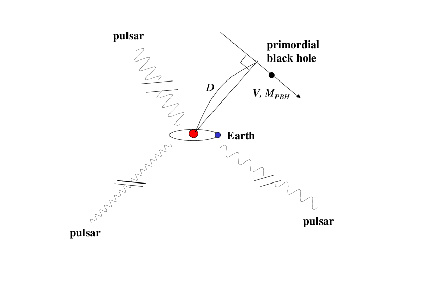
Figure 1.— Schematic picture for PBH search with pulsar timing observation. A PBH with mass $M_{\rm PBH}$ and velocity $V$ passes near the Sun with closest distance $D\gg 1$AU. We fix the velocity $V$ at its typical value 350$\rm km~{}sec^{-1}$.

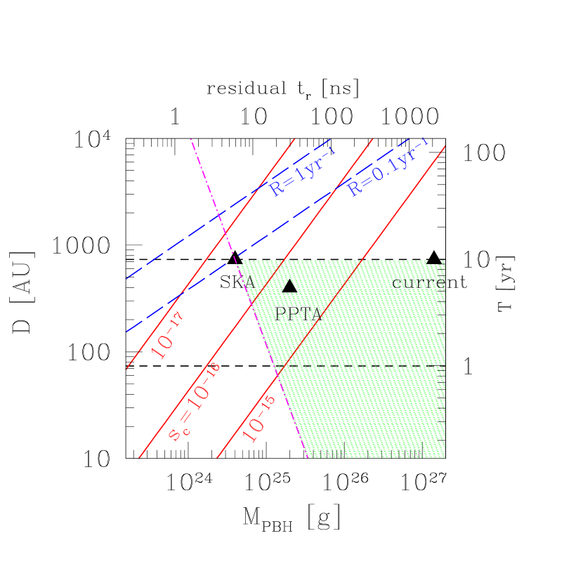
Figure 2.— Mass-distance relations under various observational conditions for PBH search. The short-dashed lines $(D\propto M_{\rm PBH}^{0})$ show the signal duration for the fixed PBH velocity $V=350$$\rm km~{}sec^{-1}$. We have one to one correspondence between the mass $M_{\rm PBH}$ (bottom axis) and the residual time $t_{r}$ (top axis). The same is true for the distance $D$ (right axis) and the time scale $T$ (left axis). The solid lines $(D\propto M_{\rm PBH}^{1})$ show the amplitudes $s_{c}$ of timing residuals in the form $\Delta\nu/\nu$. The triangles correspond to the points $(T_{\rm obs},\Omega_{GW}(T_{\rm obs}^{-1})h^{2})$ for the following three pulsar timing projects, SKA, PPTA and current results. The hatched region is detectable event for SKA bounded by the short-dashed and dash-dotted lines. The triangle for SKA moves along the dash-dotted line $(D\propto M_{\rm PBH}^{-2})$ for different observational period $T_{\rm obs}$. The long-dashed lines are distances $D$ for given event rates $R$ and mass $M_{\rm PBH}$ with putting $\rho_{\rm PBH}=\rho_{\rm DM}=0.011M_{\odot}{\rm pc^{-3}}$.

For studies involving the gravitational wave background, we often use the spectrum $\Omega_{GW}(f)\equiv\frac{1}{\rho}_{c}\frac{d\rho_{GW}(f)}{d\ln f}$ to describe the energy density of waves per logarithmic frequency interval around a frequency $f$, when normalized by the critical density $\rho_{c}$ of the universe (see e.g. Allen 1997, Maggiore 2000). The characteristic amplitude $h_{c}(T)$ is related to $\Omega_{GW}(f)$ at $T=f^{-1}$ as $\Omega_{GW}(f)=\frac{2\pi^{2}}{3H_{0}^{2}}f^{2}h_{c}(T)^{2},$ ($H_{0}=100h{\rm km~{}sec^{-1}Mpc^{-1}}$: the Hubble parameter) and we can write

$$h_{c}(T)=4.0\times 10^{-16}\left(\frac{\Omega_{GW}(f=T^{-1})h^{2}}{10^{-10}}\right)^{1/2}\left(\frac{T}{\rm 10yr}\right).$$ (6)

For a given observational period $T_{\rm obs}$, it is difficult to extract information on gravitational waves with periods longer than observational duration. This is because we cannot separate TOA residuals due to gravitational waves from secular effects such as the long-term spin evolution of pulsars (Kaspi et al. 1994, see also Damour & Taylor 1991). With the pulsar timing analysis, the sensitivity of the spectrum $\Omega_{GW}(f)$ generally becomes best at the frequency $f\simeq 1/T_{\rm obs}$ or time scale $T\simeq T_{\rm obs}$. In terms of the characteristic amplitude $h_{c}(T)$, the expected sensitivity at $T=T_{\rm obs}$ can be written with the scaling relation $h_{c}(T_{\rm obs})\propto T_{\rm obs}^{-3/2}$ (Rajagopal & Romani 1995, Jaffe & Backer 2003), with an overall normalization that depends on the parameters of the individual PTA. Similarly, we have $s_{c}(T)\propto T^{-3/2}$ or $t_{r}(T)\propto T^{-1/2}$ for the PBH acceleration with $T<T_{\rm obs}$. From eqs.(1) and (2), the above scaling relation becomes $D\propto M_{\rm PBH}^{-2}$ in the mass-distance plane.

For the present analysis the sensitivities of various pulsar timing projects can be characterized by the combination $(T_{\rm obs}$, $\Omega_{GW}(T_{\rm obs}^{-1})h^{2})$ associated with a gravitational wave background search. Here we use values $(T_{\rm obs},\Omega_{GW}(T_{\rm obs}^{-1})h^{2})=(5{\rm yr},9.1\times 10^{-11})$ for the two parameters for the PPTA following Jenet et al. (2006) ($\Omega_{GW}h^{2}$: 95% detection rate), and $(10{\rm yr},10^{-12.6})$ for the SKA-PTA from Damour and Vilenkin (2005) ($\Omega_{GW}h^{2}$: 6-$\sigma$ detection significance). As an added reference, we also take $(10{\rm yr},6.0\times 10^{-8})$ for the current observational sensitivity from Jenet et al. (2006). In Figure 2, we show the corresponding points $(T_{\rm obs},\Omega_{GW}(T_{\rm obs}^{-1})h^{2})$ as filled triangles on the mass-distance plane using eq.(6). For the SKA-PTA project, the detectable event rate is also shown as the hatched region. This region is bounded by the two lines related to the requirement $T<T_{\rm obs}$ and another related to $D\propto M_{\rm PBH}^{-2}$.

The triangle for the SKA-PTA project with $T_{\rm obs}=10$ yr is nearly on the long-dashed line $R=0.1{\rm yr^{-1}}$. This means that with $f_{\rm PBH}=1$ and $M_{\rm PBH}\sim 3\times 10^{24}$g, we will be able to detect one PBH event in a 10 yr observation with a duty cycle $C=1$. With an observational period $T_{\rm obs}$ $\sim 30$ yr, the triangle for the SKA-PTA moves upward along the dash-dotted line and is now nearly on the long-dashed line for $R=1{\rm yr^{-1}}$ and mass $M_{\rm PBH}\sim 2\times 10^{24}$g. This indicates that if the local dark matter is made by PBHs with $f_{\rm PBH}=1$ and $M_{\rm PBH}\sim 2\times 10^{24}$g, the pulse-like signals for passing PBHs with time scales $T\sim T_{\rm obs}\sim 30$ yr will highly overlap in data streams of pulsar timing.

The duty cycle $C$ is proportional to $D^{2}T/M_{\rm PBH}\propto T^{3}/M_{\rm PBH}$ for events with a time scale $T$ and a mass $M_{\rm PBH}(\propto t_{r})$. If a point in the detectable zone (the hatched region in Figure 2) on the mass-distance plane is expected to have $C>1$ as is the case for the previous example, there is an appropriate PBH mass above which the duty cycle is lower than 1, and events will be resolvable for the same time scale $T$. We can also decrease the expected duty cycle by searching shorter time-scale events and keeping the target mass $M_{\rm PBH}$. In this case the new point with $C<1$ on the plane might be out of the detectable zone after crossing the left boundary (dash-dotted line) from above.

On the other hand, if no PBH signatures are detected with the SKA-PTA in 30 yr, we can constrain their abundance fraction down to $f_{\rm PBH}\lesssim 1/10$ around $M_{\rm PBH}\sim 2\times 10^{24}$g. Of course, this is based on an order of magnitude estimate and we need detailed analysis to evaluate the exact fraction. While we have discussed the SKA-PTA so far, using the PPTA over an observational period $T_{\rm obs}$ of 5 yr, it will be difficult to detect a single PBH. With $T_{\rm obs}\sim 20$ yr, the PPTA has the potential to provide a useful constraint around $M_{\rm PBH}\sim 10^{25}$g.

3. Discussions

As we have discussed so far, it is quite important to have a long observational period $T_{\rm obs}$ and analyze long-term TOA residuals when searching for PBH signatures. For this purpose, we need stable reference clocks and high-precision ephemerides of the solar system. While we do not discuss required accuracies of them, those requirements are similar to those that are needed for gravitational wave searches (Foster & Backer 1990, Kaspi et al. 1994, Hobbs et al. 2006).

Merging super-massive black hole binaries are considered to be the dominant astrophysical source of the gravitational wave background around a frequency of $\sim 0.1{\rm yr^{-1}}$ (or a time scale $T\sim 10$ yr) (see also Damour & Vilenkin 2005 for the gravitational wave background generated by cosmic strings). The estimated amplitude using simple assumptions is $h_{c}\sim 10^{-15.5}-10^{-16}$ at $f=0.1{\rm yr^{-1}}$ (Jaffe & Backer 2003, Wyithe & Loeb 2003). But depending on model parameters, a smaller amplitude $h_{c}\sim 10^{-16.5}$ is also predicted (Enoki & Nagashima 2006). While the estimated amplitude has a large uncertainty at present, this gravitational wave background can be an effective noise for a PBH search and vice-versa. Therefore, it is desirable to observationally distinguish these two signatures in TOA residuals.

One straightforward approach is to investigate spectral information of the residuals expected for the PBH accelerations and at the same time the gravitational wave background. Another approach is to use the angular pattern of the residuals on the sky. A PBH signature will have a dipole pattern ($l=1$) whose direction is determined by the acceleration vector. In this respect the dipole component parallel to the ecliptic plane will be more affected by errors in the solar system ephemerides than the component perpendicular to the plane. On the other hand, the angular pattern due to the gravitational wave background does not have a dipole moment but has multipole modes starting from the quadrupole $(l=2)$ where 75% of the angular power is expected to exist (Burke 1975). Therefore, by studying the angular pattern of the timing residuals we can, in principle, separate the signatures of PBH events from gravitational waves. Once PTAs start to monitor sufficient pulsars, it is clear these topics must be further investigated.

NS would like to thank S. Kawamura, T. Tanaka and T. Daishido for stimulating conversations, and M. Kramer for information on SKA. We also thank an anonymous referee for detailed comments on the manuscript and J. Cooke for carefully reading the draft. This work is supported by McCue fund at UC Irvine.

References

- Adams & Bloom (2004) Adams, A. W., & Bloom, J. S. 2004, arXiv:astro-ph/0405266
- Alcock et al. (1998) Alcock, C., et al. 1998, ApJ, 499, L9
- Allen (1997) Allen, B. 1997, arXiv:gr-qc/9604033
- (4) Bender, P. L., et al. 1998, LISA Pre-Phase A Report (2d ed.; Garching: Max-Plank-Institut fur Qantenoptik)
- Bertone et al. (2005) Bertone, G., Hooper, D., & Silk, J. 2005, Phys. Rep., 405, 279
- Blandford et al. (1984) Blandford, R., Romani, R. W., & Narayan, R. 1984, Journal of Astrophysics and Astronomy, 5, 369
- Burke (1975) Burke, W. L. 1975, ApJ, 196, 329
- Carr & Sakellariadou (1999) Carr, B. J., & Sakellariadou, M. 1999, ApJ, 516, 195
- Carr (2005) Carr, B. J. 2005, arXiv:astro-ph/0511743
- Cordes et al. (2004) Cordes, J. M., et al. 2004, New Astronomy Review, 48, 1413
- Cutler & Thorne (2002) Cutler, C., & Thorne, K. S. 2002, arXiv:gr-qc/0204090
- Damour & Taylor (1991) Damour, T., & Taylor, J. H. 1991, ApJ, 366, 501
- Damour & Vilenkin (2005) Damour, T., & Vilenkin, A. 2005, Phys. Rev. D, 71, 063510
- Detweiler (1979) Detweiler, S. 1979, ApJ, 234, 1100
- Enoki & Nagashima (2006) Enoki, M., & Nagashima, M. 2006, arXiv:astro-ph/0609377
- Foster & Backer (1990) Foster, R. S., & Backer, D. C. 1990, ApJ, 361, 300
- Gould (1992) Gould, A. 1992, ApJ, 386, L5
- Hellings & Downs (1983) Hellings, R. W., & Downs, G. S. 1983, ApJ, 265, L39
- Hobbs et al. (2006) Hobbs, G. B., Edwards, R. T., & Manchester, R. N. 2006, MNRAS, 369, 655
- Inoue & Tanaka (2003) Inoue, K. T., & Tanaka, T. 2003, Phys. Rev. Lett., 91, 021101
- Ioka et al. (1998) Ioka, K., et al. 1998, Phys. Rev. D, 58, 063003
- Jaffe & Backer (2003) Jaffe, A. H., & Backer, D. C. 2003, ApJ, 583, 616
- Jenet et al. (2004) Jenet, F. A., et al. 2004, ApJ, 606, 799
- Jenet et al. (2005) Jenet, F. A., et al. 2005, ApJ, 625, L123
- Jenet et al. (2006) Jenet, F. A., et al. 2006, arXiv:astro-ph/0609013
- Kaspi et al. (1994) Kaspi, V. M., Taylor, J. H., & Ryba, M. F. 1994, ApJ, 428, 713
- Kramer et al. (2004) Kramer, M., et al. 2004, New Astronomy Review, 48, 993
- Maggiore (2000) Maggiore, M. 2000, Phys. Rep., 331, 283
- McHugh et al. (1996) McHugh, M. P., et al. 1996, Phys. Rev. D, 54, 5993
- Nakamura et al. (1997) Nakamura, T., et al. 1997, ApJ, 487, L139
- Olling & Merrifield (2001) Olling, R. P., & Merrifield, M. R. 2001, MNRAS, 326, 164
- Rajagopal & Romani (1995) Rajagopal, M., & Romani, R. W. 1995, ApJ, 446, 543
- Seto & Cooray (2004) Seto, N., & Cooray, A. 2004, Phys. Rev. D, 70, 063512
- Thorsett & Dewey (1996) Thorsett, S. E., & Dewey, R. J. 1996, Phys. Rev. D, 53, 3468
- Wyithe & Loeb (2003) Wyithe, J. S. B., & Loeb, A. 2003, ApJ, 590, 691
- Zakamska & Tremaine (2005) Zakamska, N. L., & Tremaine, S. 2005, AJ, 130, 1939