SDSS galaxy clustering: luminosity and colour dependence and stochasticity

Abstract

Differences in clustering properties between galaxy subpopulations complicate the cosmological interpretation of the galaxy power spectrum, but can also provide insights about the physics underlying galaxy formation. To study the nature of this relative clustering, we perform a counts-in-cells analysis of galaxies in the Sloan Digital Sky Survey (SDSS) in which we measure the relative bias between pairs of galaxy subsamples of different luminosities and colours. We use a generalized $\chi^{2}$ test to determine if the relative bias between each pair of subsamples is consistent with the simplest deterministic linear bias model, and we also use a maximum likelihood technique to further understand the nature of the relative bias between each pair. We find that the simple, deterministic model is a good fit for the luminosity-dependent bias on scales above $\sim 2\,h^{-1}\mathrm{Mpc}$, which is good news for using magnitude-limited surveys for cosmology. However, the colour-dependent bias shows evidence for stochasticity and/or non-linearity which increases in strength toward smaller scales, in agreement with previous studies of stochastic bias. Also, confirming hints seen in earlier work, the luminosity-dependent bias for red galaxies is significantly different from that of blue galaxies: both luminous and dim red galaxies have higher bias than moderately bright red galaxies, whereas the biasing of blue galaxies is not strongly luminosity-dependent. These results can be used to constrain galaxy formation models and also to quantify how the colour and luminosity selection of a galaxy survey can impact measurements of the cosmological matter power spectrum.

1 Introduction

In order to use galaxy surveys to study the large-scale distribution of matter, the relation between the galaxies and the underlying matter – known as the galaxy bias – must be understood. Developing a detailed understanding of this bias is important for two reasons: bias is a key systematic uncertainty in the inference of cosmological parameters from galaxy surveys, and it also has implications for galaxy formation theory.

Since it is difficult to measure the dark matter distribution directly, we can gain insight by studying relative bias, i.e., the relation between the spatial distributions of different galaxy subpopulations. There is a rich body of literature on this subject tracing back many decades (see, e.g., Hubble & Humason 1931; Davis & Geller 1976; Hamilton 1988; White et al. 1988; Park et al. 1994; Loveday et al. 1995), and been studied extensively in recent years as well, both theoretically (Seljak, 2001; van den Bosch et al., 2003; Cooray, 2005; Sheth et al., 2005; Tinker et al., 2007) and observationally. Such studies have established that biasing depends on the type of galaxy under consideration – for example, early-type, red galaxies are more clustered than late-type, blue galaxies (Guzzo et al., 1997; Norberg et al., 2002; Madgwick et al., 2003; Conway et al., 2005; Li et al., 2006; Croton et al., 2007), and luminous galaxies are more clustered than dim galaxies (Willmer et al., 1998; Norberg et al., 2001; Tegmark et al., 2004b; Zehavi et al., 2005; Seljak et al., 2005; Skibba et al., 2006). Since different types of galaxies do not exactly trace each other, it is thus impossible for them all to be exact tracers of the underlying matter distribution.

More quantitatively, the luminosity dependence of bias has been measured in the 2 Degree Field Galaxy Redshift Survey (2dFGRS; Colless et al. 2001) (Norberg et al., 2001, 2002) and in the Sloan Digital Sky Survey (SDSS; York et al. 2000; Stoughton et al. 2002) (Tegmark et al., 2004b; Zehavi et al., 2005; Li et al., 2006) as well as other surveys, and it is generally found that luminous galaxies are more strongly biased, with the difference becoming more pronounced above $L_{*}$, the characteristic luminosity of a galaxy in the Schechter luminosity function (Schechter, 1976).

These most recent studies measured the bias from ratios of correlation functions or power spectra. The variances of clustering estimators like correlation functions and power spectra are well-known to be the sum of two physically separate contributions: Poisson shot noise (due to the sampling of the underlying continuous density field with a finite number of galaxies) and sample variance (due to the fact that only a finite spatial volume is probed). On the large scales most relevant to cosmological parameter studies, sample variance dominated the aforementioned 2dFGRS and SDSS measurements, and therefore dominated the error bars on the inferred bias.

This sample variance is easy to understand: if the power spectrum of distant luminous galaxies is measured to be different than that of nearby dim galaxies, then part of this measured bias could be due to the nearby region happening to be more/less clumpy than the distant one. In this paper, we will eliminate this annoying sample variance by comparing how different galaxies cluster in the same region of space, extending the counts-in-cells work of Tegmark & Bromley (1999), Blanton (2000), and Wild et al. (2005) and the correlation function work of Norberg et al. (2001), Norberg et al. (2002), Zehavi et al. (2005), and Li et al. (2006). Here we use the counts-in-cells technique: we divide the survey volume into roughly cubical cells and compare the number of galaxies of each type within each cell. This yields a local, point-by-point measure of the relative bias rather than a global one as in the correlation function method. In other words, by comparing two galaxy density fields directly in real space, including the phase information that correlation function and power spectrum estimators discard, we are able to provide substantially sharper bias constraints.

This local approach also enables us to quantify so-called stochastic bias (Pen, 1998; Tegmark & Peebles, 1998; Dekel & Lahav, 1999; Matsubara, 1999). It is well-known that the relation between galaxies and dark matter or between two different types of galaxies is not necessarily deterministic – galaxy formation processes that depend on variables other than the local matter density give rise to stochastic bias as described in Pen (1998), Tegmark & Peebles (1998), Dekel & Lahav (1999), and Matsubara (1999). Evidence for stochasticity in the relative bias between early-type and late-type galaxies has been presented in Wild et al. (2005), Conway et al. (2005), Tegmark & Bromley (1999), and Blanton (2000). Additionally, Simon et al. (2007) finds evidence for stochastic bias between galaxies and dark matter via weak lensing. The time evolution of such stochastic bias has been modelled in Tegmark & Peebles (1998) and was recently updated in Simon (2005). Stochasticity is even predicted in the relative bias between virialized clumps of dark matter (haloes) and the linearly-evolved dark matter distribution (Casas-Miranda et al., 2002; Seljak & Warren, 2004). Here we aim to test whether stochasticity is necessary for modelling the luminosity-dependent or the colour-dependent relative bias.

In this paper, we study the relative bias as a function of scale using a simple stochastic biasing model by comparing pairs of SDSS galaxy subsamples in cells of varying size. Such a study is timely for two reasons. First of all, the galaxy power spectrum has recently been measured to high precision on large scales with the goal of constraining cosmology (Tegmark et al., 2004b, 2006; Blake et al., 2007; Padmanabhan et al., 2007). As techniques continue to improve and survey volumes continue to grow, it is necessary to reduce systematic uncertainties in order to keep pace with shrinking statistical uncertainties. A detailed understanding of complications due to the dependence of galaxy bias on scale, luminosity, and colour will be essential for making precise cosmological inferences with the next generation of galaxy redshift surveys (Percival et al., 2004; Abazajian et al., 2005; Percival et al., 2007; Zheng & Weinberg, 2007; Möller et al., 2007; Kristiansen et al., 2007).

Secondly, a great deal of theoretical progress on models of galaxy formation has been made in recent years, and 2dFGRS and SDSS contain a large enough sample of galaxies that we can now begin to place robust and detailed observational constraints on these models. The framework known as the halo model (Seljak, 2000) (see Cooray & Sheth 2002 for a comprehensive review) provides the tools needed to make comparisons between theory and observations. The halo model assumes that all galaxies form in dark matter haloes, so the galaxy distribution can be modelled by first determining the halo distribution – either analytically (Catelan et al., 1998; McDonald, 2006; Smith et al., 2007) or using $N$-body simulations (Smith et al., 2003; Kravtsov et al., 2004; Kravtsov, 2006) – and then populating the haloes with galaxies. This second step can be done using semi-analytical galaxy formation models (Somerville et al., 2001; Berlind et al., 2003; Croton et al., 2006; Baugh, 2006) or with a statistical approach using a model for the halo occupation distribution (HOD) (Peacock & Smith, 2000; Berlind & Weinberg, 2002; Sefusatti & Scoccimarro, 2005) or conditional luminosity function (CLF) (Yang et al., 2003; van den Bosch et al., 2003) which prescribes how galaxies populate haloes.

Although there are some concerns that the halo model does not capture all of the relevant physics (Yang et al., 2006; Cooray, 2006; Gao & White, 2007), it has been applied successfully in a number of different contexts (Scranton, 2003; Collister & Lahav, 2005; Tinker et al., 2006; Skibba et al., 2006). The correlation between a galaxy’s environment (i.e., the local density of surrounding galaxies) and its colour and luminosity (Hogg et al. 2004; Blanton et al. 2005a) has been interpreted in the context of the halo model (Berlind et al., 2005; Blanton et al., 2006; Abbas & Sheth, 2006), and van den Bosch et al. (2003) and Cooray (2005) make predictions for the bias as a function of galaxy type and luminosity using the CLF formalism. Additionally, Zehavi et al. (2005), Magliocchetti & Porciani (2003), and Abbas & Sheth (2005) use correlation function methods to study the luminosity and colour dependence of galaxy clustering, and interpret the results using the Halo Occupation Distribution (HOD) framework. The analysis presented here is complementary to this body of work in that the counts-in-cells method is sensitive to larger scales, uses a different set of assumptions, and compares the two density fields directly in each cell rather than comparing ratios of their second moments. The halo model provides a natural framework in which to interpret the luminosity and colour dependence of galaxy biasing statistics we measure here.

The rest of this paper is organized as follows: Section 2 describes our galaxy data, and Sections 3.1 and 3.2 describe the construction of our galaxy samples and the partition of the survey volume into cells. In Section 3.3 we outline our relative bias framework, and in Sections 3.4 and 3.5 we describe our two main analysis methods. We present our results in Section 4 and conclude with a qualitative interpretation of our results in the halo model context in Section 5.

2 SDSS Galaxy Data

The SDSS (York et al., 2000; Stoughton et al., 2002) uses a mosaic CCD camera (Gunn et al., 1998) on a dedicated telescope (Gunn et al., 2006) to image the sky in five photometric bandpasses denoted $u$, $g$, $r$, $i$ and $z$ (Fukugita et al., 1996). After astrometric calibration (Pier et al., 2003), photometric data reduction (Lupton et al., 2001), and photometric calibration (Hogg et al., 2001; Smith et al., 2002; Ivezić et al., 2004; Tucker et al., 2006), galaxies are selected for spectroscopic observations. To a good approximation, the main galaxy sample consists of all galaxies with $r$-band apparent Petrosian magnitude $r<17.77$ after correction for reddening as per Schlegel et al. (1998); there are about 90 such galaxies per square degree, with a median redshift of 0.1 and a tail out to $z\sim 0.25$. Galaxy spectra are also measured for the Luminous Red Galaxy sample (Eisenstein et al., 2001), which is not used in this paper. These targets are assigned to spectroscopic plates of diameter $2.98^{\circ}$ by an adaptive tiling algorithm (Blanton et al. 2003b) and observed with a pair of CCD spectrographs (Uomoto et al., 2004), after which the spectroscopic data reduction and redshift determination are performed by automated pipelines. The rms galaxy redshift errors are of order $30\,\mathrm{km\,s^{-1}}$ for main galaxies, hence negligible for the purposes of the present paper.

Our analysis is based on 380,614 main galaxies (the ‘safe0’ cut) from the 444,189 galaxies in the 5th SDSS data release (‘DR5’) (Adelman-McCarthy et al., 2007), processed via the SDSS data repository at New York University (Blanton et al. 2005b). The details of how these samples were processed and modelled are given in Appendix A of Tegmark et al. (2004b) and in Eisenstein et al. (2005). The bottom line is that each sample is completely specified by three entities:

1. The galaxy positions (RA, Dec, and comoving redshift space distance $r$ for each galaxy) ;

2. The radial selection function $\bar{n}\left(r\right)$, which gives the expected (not observed) number density of galaxies as a function of distance ;

3. The angular selection function $\bar{n}\left(\hat{\mn@boldsymbol{r}}\right)$, which gives the completeness as a function of direction in the sky, specified in a set of spherical polygons (Hamilton & Tegmark, 2004).

The three-dimensional selection functions of our samples are separable, i.e., simply the product $\bar{n}\left(\mn@boldsymbol{r}\right)=\bar{n}\left(\hat{\mn@boldsymbol{r}}\right)\bar{n}\left(r\right)$ of an angular and a radial part; here $r\equiv|\mn@boldsymbol{r}|$ and $\hat{\mn@boldsymbol{r}}\equiv\mn@boldsymbol{r}/r$ are the radial comoving distance and the unit vector corresponding to the position $\mn@boldsymbol{r}$. The volume-limited samples used in this paper are constructed so that their radial selection function $\bar{n}\left(r\right)$ is constant over a range of $r$ and zero elsewhere. The effective sky area covered is $\Omega\equiv\int\bar{n}\left(\hat{\mn@boldsymbol{r}}\right)d\Omega\approx 5183$ square degrees, and the typical completeness $\bar{n}\left(\hat{\mn@boldsymbol{r}}\right)$ exceeds 90 per cent. The conversion from redshift $z$ to comoving distance was made for a flat $\Lambda\mathrm{CDM}$ cosmological model with $\Omega_{m}=0.25$. Additionally, we make a first-order correction for redshift space distortions by applying the finger-of-god compression algorithm described in Tegmark et al. (2004b) with a threshold density of $\delta_{c}=200$.

3 Analysis Methods

3.1 Overlapping Volume-Limited Samples

The basic technique used in this paper is pairwise comparison of the three-dimensional density fields of galaxy samples with different colours and luminosities. As in Zehavi et al. (2005), we focus on these two properties (as opposed to morphological type, spectral type, or surface brightness) for two reasons: they are straightforward to measure from SDSS data, and recent work (Blanton et al. 2005a) has found that luminosity and colour is the pair of properties that is most predictive of the local overdensity. Since colour and spectral type are strongly correlated, our study of the colour dependence of bias probes similar physics as studies using spectral type (Tegmark & Bromley, 1999; Blanton, 2000; Norberg et al., 2002; Wild et al., 2005; Conway et al., 2005).

Our base sample of SDSS galaxies (‘safe0’) has an $r$-band apparent magnitude range of $14.5<r<17.5$. Following the method used in Tegmark et al. (2004b), we created a series of volume-limited samples containing galaxies in different luminosity ranges. These samples are defined by selecting a range of absolute magnitude $M_{\mathrm{luminous}}<M_{{}^{0.1}r}<M_{\mathrm{dim}}$ and defining a redshift range such that the near limit has $M_{{}^{0.1}r}=M_{\mathrm{luminous}}$, $r=14.5$ and the far limit has $M_{{}^{0.1}r}=M_{\mathrm{dim}}$, $r=17.5$. Thus by discarding all galaxies outside the redshift range, we are left with a sample with a uniform radial selection function $\bar{n}\left(r\right)$ that contains all of the galaxies in the given absolute magnitude range in the volume defined by the redshift limits. Here $M_{{}^{0.1}r}$ is defined as the absolute magnitude in the $r$-band shifted to a redshift of $z=0.1$ (Blanton et al. 2003a).

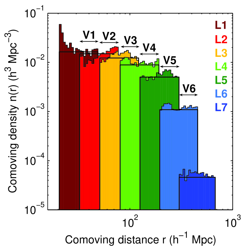
Figure 1: Histogram of the comoving number density (after finger-of-god compression) of the volume-limited samples L1-L7. The cuts used to define these samples are shown in Table 1. Note that the radial selection function $\bar{n}\left(r\right)$ is uniform over the allowed range for each sample. Arrows indicate volumes V1-V6 where neighbouring volume-limited samples overlap.

Our volume-limited samples are labelled L1 through L7, with L1 being the dimmest and L7 being the most luminous. Figure 1 shows a histogram of the comoving galaxy density $n\left(r\right)$ for L1-L7. The cuts used to make these samples are shown in Table 1.

Table 1: Summary of cuts used to create luminosity-binned volume-limited samples.

Luminosity-binned			Comoving number
volume-limited samples	Absolute magnitude	Redshift	density $\bar{n}$ $\left(h^{3}{\mathrm{Mpc}}^{-3}\right)$
L1	$-17<M_{{}^{0.1}r}<-16$	$0.007<z<0.016$	$\left(1.63\pm 0.05\right)\times 10^{-2}$
L2	$-18<M_{{}^{0.1}r}<-17$	$0.011<z<0.026$	$\left(1.50\pm 0.03\right)\times 10^{-2}$
L3	$-19<M_{{}^{0.1}r}<-18$	$0.017<z<0.041$	$\left(1.23\pm 0.01\right)\times 10^{-2}$
L4	$-20<M_{{}^{0.1}r}<-19$	$0.027<z<0.064$	$\left(8.86\pm 0.05\right)\times 10^{-3}$
L5	$-21<M_{{}^{0.1}r}<-20$	$0.042<z<0.100$	$\left(5.02\pm 0.02\right)\times 10^{-3}$
L6	$-22<M_{{}^{0.1}r}<-21$	$0.065<z<0.152$	$\left(1.089\pm 0.005\right)\times 10^{-3}$
L7	$-23<M_{0.1_{r}}<-22$	$0.101<z<0.226$	$\left(4.60\pm 0.06\right)\times 10^{-5}$

Each sample overlaps spatially only with the samples in neighbouring luminosity bins – since the apparent magnitude range spans three magnitudes and the absolute magnitude ranges for each bin span one magnitude, the far redshift limit of a given luminosity bin is approximately equal to the near redshift limit of the bin two notches more luminous. (It is not precisely equal due to evolution and K-corrections.)

The regions where neighbouring volume-limited samples overlap provide a clean way to select data for studying the luminosity-dependent bias. By using only the galaxies in the overlapping region from each of the two neighbouring luminosity bins, we obtain two sets of objects (one from the dimmer bin and one from more luminous bin) whose selection is volume-limited and redshift-independent. Furthermore, since they occupy the same volume, they are correlated with the same underlying matter distribution, which eliminates uncertainty due to sample variance and removes potential systematic effects due to sampling different volume sizes (Joyce et al., 2005). We label the overlapping volume regions V1 through V6, where V1 is defined as the overlap between L1 and L2, and so forth. The redshift ranges for V1-V6 are shown Table 2.

Table 2: Overlapping volumes in which neighbouring luminosity bins are compared.

Pairwise comparison	Overlapping
(overlapping) volumes	bins	Redshift
V1	L1 & L2	$0.011<z<0.016$
V2	L2 & L3	$0.017<z<0.026$
V3	L3 & L4	$0.027<z<0.041$
V4	L4 & L5	$0.042<z<0.064$
V5	L5 & L6	$0.065<z<0.100$
V6	L6 & L7	$0.101<z<0.152$

To study the colour dependence of the bias, we further divide each sample into red galaxies and blue galaxies. Figure 2 shows the galaxy distribution of our volume-limited samples on a colour-magnitude diagram. The sharp boundaries between the different horizontal slices are due to the differences in density and total volume sampled in each luminosity bin. This diagram illustrates the well-known colour bimodality, with the redder galaxies falling predominantly in a region commonly known as the E-S0 ridgeline (Balogh et al., 2004; Mateus et al., 2006; Baldry et al., 2006). To separate the E-S0 ridgeline from the rest of the population, we use the same magnitude-dependent colour cut as in Zehavi et al. (2005): we define galaxies with ${}^{0.1}\left(g-r\right)<0.9-0.03\left(M_{{}^{0.1}r}+23\right)$ to be blue and galaxies on the other side of this line to be red.

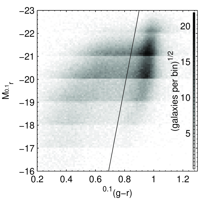
Figure 2: Colour-magnitude diagram showing the number density distribution of the galaxies in the volume-limited samples. The shading scale has a square-root stretch, with darker areas indicating regions of higher density. The line shows the colour cut of ${}^{0.1}\left(g-r\right)=0.9-0.03\left(M_{{}^{0.1}r}+23\right)$. We refer to galaxies falling to the left of this line as blue and ones falling to the right of the line as red.

In each volume V1-V6, we make four separate pairwise comparisons: luminous galaxies vs. dim galaxies, red galaxies vs. blue galaxies, luminous red galaxies vs. dim red galaxies, and luminous blue galaxies vs. dim blue galaxies. The luminous vs. dim comparisons measures the relative bias between galaxies in neighbouring luminosity bins, and from this we can extract the luminosity dependence of the bias for all galaxies combined and for red and blue galaxies separately. The red vs. blue comparison measures the colour-dependent bias. This set of four different types of pairwise comparisons is illustrated in Fig. 3 for V4, and the number of galaxies in each sample being compared is shown in Table 3.

Table 3: Number of galaxies in each sample being compared.

	All split by luminosity		All split by colour
	Luminous	Dim	Red	Blue
V1	427	651	125	953
V2	2102	2806	1117	3791
V3	6124	8273	5147	9250
V4	12122	23534	17144	18512
V5	11202	53410	37472	27140
V6	1784	38920	27138	13566
	Red split by luminosity		Blue split by luminosity
	Red luminous	Red dim	Blue luminous	Blue dim
V1	72	53	355	598
V2	620	497	1482	2309
V3	2797	2350	3327	5923
V4	6848	10296	5274	13238
V5	7514	29958	3688	23452
V6	1451	25687	333	13233

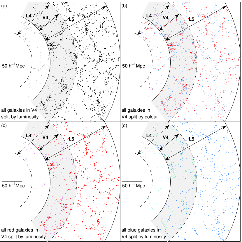
Figure 3: Galaxy distributions (after finger-of-god compression) plotted in comoving spatial co-ordinates for a radial slice of the volume-limited samples L4 (smaller dots, radial boundaries denoted by dashed lines) and L5 (larger dots, radial boundaries denoted by solid lines), which overlap in volume V4. Four different types of pairwise comparisons are illustrated: (a) luminous galaxies (L5) vs. dim galaxies (L4), (b) red galaxies vs. blue galaxies (both in V4), (c) luminous red galaxies (L5) vs. dim red galaxies (L4), and (d) luminous blue galaxies (L5) vs. dim blue galaxies (L4). The shaded regions denote the volume in which the two sets of galaxies are compared. A simple visual inspection shows that the different samples of galaxies being compared generally appear to cluster in the same physical locations – one key question we aim to answer here is if these observed correlations can be described with a simple linear bias model.

3.2 Counts-in-Cells Methodology

To compare the different pairs of galaxy samples, we perform a counts-in-cells analysis: we divide each comparison volume into roughly cubical cells and use the number of galaxies of each type in each cell as the primary input to our statistical analysis. This method is complementary to studies based on the correlation function since it involves point-by-point comparison of the two density fields and thus provides a more direct test of the local deterministic linear bias hypothesis. We probe scale dependence by varying the size of the cells.

To create our cells, we first divide the sky into two-dimensional ‘pixels’ at four different angular resolutions using the SDSSPix pixelization scheme as implemented by an updated version of the angular mask processing software mangle (Hamilton & Tegmark, 2004; Swanson et al., 2007). The angular selection function $\bar{n}\left(\hat{\mn@boldsymbol{r}}\right)$ is averaged over each pixel to obtain the completeness. To reduce the effects of pixels on the edge of the survey area or in regions affected by internal holes in the survey, we apply a cut on pixel completeness: we only use pixels with a completeness higher than 80 per cent (50 per cent for the lowest angular resolution). Figure 4 shows the pixelized SDSS angular mask at our four different resolutions, including only the pixels that pass our completeness cut. The different angular resolutions have 15, 33, 157, and 901 of these angular pixels respectively. At the lowest resolution, each pixel covers 353 square degrees, and the angular area of the pixels decreases by a factor of $1/4$ at each resolution level, yielding pixels covering 88, 22, and 5 square degrees at the three higher resolutions.

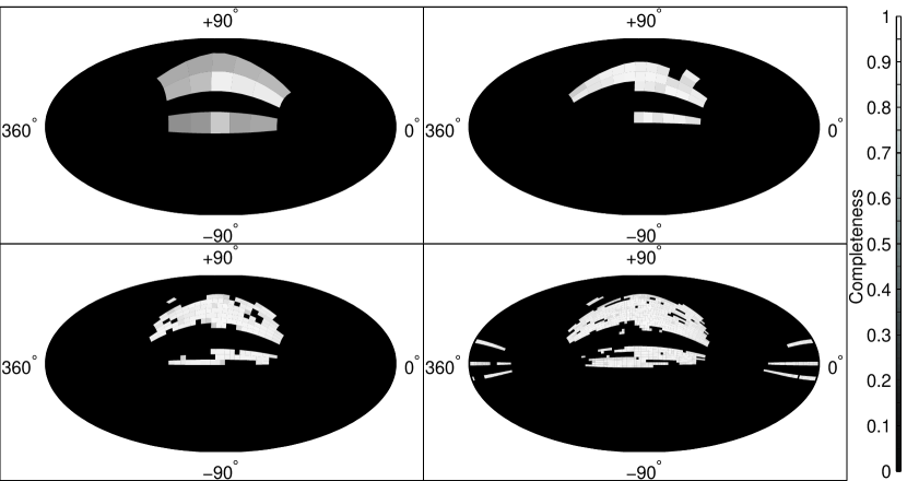
Figure 4: The SDSS DR5 angular mask pixelized at the four different resolutions used to partition the survey into cells, shown in Hammer-Aitoff projection in equatorial co-ordinates. Shading indicates completeness level: 0 per cent is black, 100 per cent is white.

To produce three-dimensional cells from our pixels, we divide each comparison volume into radial shells of equal volume. We choose the number of radial subdivisions at each angular resolution in each comparison volume such that our cells are approximately cubical, i.e., the radial extent of a cell is approximately equal to its transverse (angular) extent. This procedure makes cells that are not quite perfect cubes – there is some slight variation in the cell shapes, with cells on the near edge of the volume slightly elongated radially and cells on the far edge slightly flattened. We state all of our results as a function of cell size $L$, defined as the cube root of the cell volume. At the lowest resolution, there is just 1 radial shell for each volume; at the next resolution, we have 3 radial shells for volumes V4 and V5 and 2 radial shells for the other volumes. There are 5 radial shells at the second highest resolution, and 10 at the highest.

Since each comparison volume is at a different distance from us, the angular geometry gives us cells of different physical size in each of the volumes. At the lowest resolution, where there is only one shell in each volume, the cell size is $14\,h^{-1}\mathrm{Mpc}$ in V1 and $134\,h^{-1}\mathrm{Mpc}$ in V6. At the highest resolution, the cell size is $1.7\,h^{-1}\mathrm{Mpc}$ in V1 and $16\,h^{-1}\mathrm{Mpc}$ in V6. Figure 5 shows the cells in each volume V1-V6 that are closest to a size of $\sim 20{\,h}^{-1}\mathrm{Mpc}$, the range in which the length scales probed by the different volumes overlap. (These are the cells used to produce the results shown in Fig. 8.)

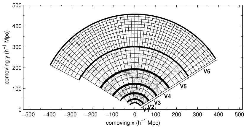
Figure 5: A radial slice of the SDSS survey volume divided into cells of size $\sim 20{\,h}^{-1}\mathrm{Mpc}$ with the galaxies in each cell (after finger-of-god compression) shown in grey.

3.3 Relative Bias Framework

Our task is to quantify the relationship between two fractional overdensity fields $\delta_{1}\left(\mn@boldsymbol{x}\right)\equiv\rho_{1}\left(\mn@boldsymbol{x}\right)/\bar{\rho}_{1}-1$ and $\delta_{2}\left(\mn@boldsymbol{x}\right)\equiv\rho_{2}\left(\mn@boldsymbol{x}\right)/\bar{\rho}_{2}-1$ representing two different types of objects. This framework is commonly used with types (1,2) representing (dark matter, galaxies), or as in Blanton (2000), Wild et al. (2005), and Conway et al. (2005), (early-type galaxies, late-type galaxies). Here we use it to represent (more luminous galaxies, dimmer galaxies) or (red galaxies, blue galaxies) to compare the samples described in Section 3.1. Galaxies are of course discrete objects, and as customary, we use the continuous field $\rho_{\alpha}\left(\mn@boldsymbol{x}\right)$ (where $\alpha$=1 or 2) to formally refer to the expectation value of the Poisson point process involved in distributing the type $\alpha$ galaxies.

The simplest (and frequently assumed) relationship between $\delta_{1}$ and $\delta_{2}$ is linear deterministic bias:

$$\delta_{2}\left(\mn@boldsymbol{x}\right)=b_{\mathrm{lin}}\delta_{1}\left(\mn@boldsymbol{x}\right),$$ (1)

where $b_{\mathrm{lin}}$ is a constant parameter. This model cannot hold in all cases – note that it can give negative densities if $b_{\mathrm{lin}}>1$ – but is typically a reasonable approximation on cosmologically large length scales where the density fluctuations $\delta_{1}\ll 1$, as is the case for the measurements of the large scale power spectrum recently used to constrain cosmological parameters (Tegmark et al., 2004b; Cole et al., 2005; Tegmark et al., 2006)

More complicated models allow for non-linearity and stochasticity, as described in detail in Dekel & Lahav (1999):

$$\delta_{2}\left(\mn@boldsymbol{x}\right)=b\left[\delta_{1}\left(\mn@boldsymbol{x}\right)\right]\delta_{1}\left(\mn@boldsymbol{x}\right)+\epsilon\left(\mn@boldsymbol{x}\right),$$ (2)

where the bias $b$ is now a (typically slightly non-linear) function of $\delta_{1}$. The stochasticity is represented by a random field $\epsilon$ – allowing for stochasticity removes the restriction implied by deterministic models that the peaks of $\delta_{1}$ and $\delta_{2}$ must coincide spatially. Stochasticity is basically the scatter in the relationship between the two density fields due to physical variables besides the local matter density. Non-local galaxy formation processes can also give rise to stochasticity, as discussed in Matsubara (1999).

We estimate the overdensity of galaxies of type $\alpha$ in cell $i$ by

$$g_{\alpha}^{(i)}\equiv\frac{N_{\alpha}^{(i)}-\bar{N}_{\alpha}^{(i)}}{\bar{N}_{\alpha}^{(i)}},$$ (3)

where $N_{\alpha}^{(i)}$ is the number of observed type $\alpha$ galaxies in cell $i$ and $\bar{N}_{\alpha}^{(i)}$ is the expected number of such galaxies, computed from the average angular selection function in the pixel and normalized so that the sum of $\bar{N}_{\alpha}^{(i)}$ over all cells in the comparison volume matches the total number of observed type $\alpha$ galaxies. The $n$-dimensional vectors

$${\mn@boldsymbol{g}}_{\alpha}\equiv\left(\begin{array}[]{c}g_{\alpha}^{(1)}\\ \vdots\\ g_{\alpha}^{(n)}\end{array}\right)$$ (4)

contain the counts-in-cells data to which we apply the statistical analyses in Sections 3.4 and 3.5.

The covariance matrix of $\mn@boldsymbol{g}$ is given by

$$\left\langle g_{\alpha}^{(i)}g_{\beta}^{(j)}\right\rangle=\left\langle\delta_{\alpha}^{(i)}\delta_{\beta}^{(j)}\right\rangle+\delta_{\alpha\beta}{\textbf{{N}}}_{\alpha}^{ij},$$ (5)

where $\delta_{\alpha}^{(i)}$ is the average of $\delta_{\alpha}\left(\mn@boldsymbol{x}\right)$ over cell $i$ and, making the customary assumption that the shot noise is Poissonian, the shot noise covariance matrix ${\textbf{{N}}}_{\alpha}$ is given by

$${\textbf{{N}}}_{\alpha}^{ij}\equiv\delta_{ij}/\bar{N}_{\alpha}^{(i)}.$$ (6)

For comparing pairs of different types of galaxies, we construct the data vector

$$\mn@boldsymbol{g}\equiv\left(\begin{array}[]{c}{\mn@boldsymbol{g}}_{1}\\ {\mn@boldsymbol{g}}_{2}\end{array}\right),$$ (7)

which has a covariance matrix

$$\textbf{{C}}\equiv\left\langle\mn@boldsymbol{g}{\mn@boldsymbol{g}}^{T}\right\rangle=\textbf{{S}}+\textbf{{N}},$$ (8)

with

$$\textbf{{N}}\equiv\left(\begin{array}[]{cc}{\textbf{{N}}}_{1}&0\\ 0&{\textbf{{N}}}_{2}\end{array}\right),\qquad\textbf{{S}}\equiv\left(\begin{array}[]{cc}{\textbf{{S}}}_{11}&{\textbf{{S}}}_{12}\\ {\textbf{{S}}}_{12}&{\textbf{{S}}}_{22}\end{array}\right),$$ (9)

and the elements of the matrix S given by

$${\textbf{{S}}}_{\alpha\beta}^{ij}=\left\langle\delta_{\alpha}^{(i)}\delta_{\beta}^{(j)}\right\rangle.$$ (10)

The diagonal form of N in equation (9) assumes that there are no correlations between the shot noise of type 1 and type 2 galaxies within a given cell $i$ – this means that the two galaxy distributions are treated as independent Poisson processes that sample related density distributions $\delta_{1}\left(\mn@boldsymbol{x}\right)$ and $\delta_{2}\left(\mn@boldsymbol{x}\right)$. Although one might expect the fact that the counts of type 1 and type 2 galaxies in a cell is constrained to be equal to the total number of galaxies in the cell could induce correlations in the shot noise, we do not explicitly use the combined total count in our analyses – uncorrelated shot noise is thus a reasonable assumption.

Regarding the matrix S, other counts-in-cells analyses often assume that the correlations between different cells can be ignored, i.e., $\left\langle\delta_{\alpha}^{(i)}\delta_{\beta}^{(j)}\right\rangle=0$ unless $i=j$. Here we account for cosmological correlations by computing the elements of S using the best-fitting $\Lambda$CDM matter power spectrum as we will now describe in detail. The power spectrum $P_{\alpha\beta}\left(\mn@boldsymbol{k}\right)$ is defined as $\left\langle\hat{\delta}_{\alpha}\left(\mn@boldsymbol{k}\right)\hat{\delta}_{\beta}\left({\mn@boldsymbol{k}}^{\prime}\right)^{\dagger}\right\rangle=\left(2\pi\right)^{3}\delta^{D}\left(\mn@boldsymbol{k}-{\mn@boldsymbol{k}}^{\prime}\right)P_{\alpha\beta}\left(\mn@boldsymbol{k}\right)$, where $\hat{\delta}_{\alpha}\left(\mn@boldsymbol{k}\right)\equiv\int e^{-i\mn@boldsymbol{k}\cdot\mn@boldsymbol{x}}\delta_{\alpha}\left(\mn@boldsymbol{x}\right)d^{3}\mn@boldsymbol{x}$ is the Fourier transform of the overdensity field. $P_{11}\left(\mn@boldsymbol{k}\right)$ and $P_{22}\left(\mn@boldsymbol{k}\right)$ are the power spectra of type 1 and 2 galaxies respectively, and $P_{12}\left(\mn@boldsymbol{k}\right)$ is the cross spectrum between type 1 and 2 galaxies. We assume isotropy and homogeneity, so that $P_{\alpha\beta}\left(\mn@boldsymbol{k}\right)$ is a function only of $k\equiv\left|\mn@boldsymbol{k}\right|$, and rewrite the galaxy power spectra in terms of the matter power spectrum $P\left(k\right)$:

$$P_{11}\left(k\right) = b_{1}\left(k\right)^{2}P\left(k\right)$$

$$P_{12}\left(k\right) = {b_{1}\left(k\right)b}_{2}\left(k\right)r_{12}\left(k\right)P\left(k\right)$$

$$P_{22}\left(k\right) = b_{2}\left(k\right)^{2}P\left(k\right),$$ (11)

which defines the functions $b_{1}\left(k\right)$, $b_{2}\left(k\right)$, and $r_{12}\left(k\right)$.

To calculate $\left\langle\delta_{\alpha}^{(i)}\delta_{\beta}^{(j)}\right\rangle$ exactly, we need to convolve $\delta_{\alpha}(\mn@boldsymbol{x})$ with a filter representing cell $i$ and $\delta_{\beta}(\mn@boldsymbol{x})$ with a filter representing cell $j$. This is complicated since our cells, while all roughly cubical, have slightly different shapes. We therefore use an approximation of a spherical top hat smoothing filter with radius $R$: $w\left(r,R\right)\equiv 3/(4\pi R^{3})\Theta(R-r)$ with the Fourier transform given by

$$\hat{w}\left(k,R\right)=\frac{3}{\left(kR\right)^{3}}\left[\sin\left(kR\right)-kR\cos\left(kR\right)\right].$$ (12)

$R$ is chosen so that the effective scale corresponds to cubes with side length $L$: $R=\sqrt{5/12}L$, where $L$ is the cell size defined in Section 3.2. (See p. 500 in Peacock 1999 for derivation of the $\sqrt{5/12}$ factor.) This gives

$$\left\langle\delta_{\alpha}^{(i)}\delta_{\beta}^{(j)}\right\rangle=\frac{1}{2\pi^{2}}\int_{0}^{\infty}\frac{\sin\left(kr_{ij}\right)}{kr_{ij}}P_{\alpha\beta}\left(k\right)\left|\hat{w}\left(k,R\right)\right|^{2}k^{2}{\rm{d}k,}$$ (13)

where $r_{ij}$ is the distance between the centres of cells $i$ and $j$. The kernel of this integrand – meaning everything besides $P_{\alpha\beta}\left(k\right)$ here – typically peaks at $k\sim 1/R$ and is only non-negligible in a range of $\Delta\log_{10}k\sim 1$. Assuming that the functions $b_{1}\left(k\right)$, $b_{2}\left(k\right)$, and $r_{12}\left(k\right)$ vary slowly with $k$ over this range, they can be approximated by their values at $k_{\mathrm{peak}}\equiv 1/R=\sqrt{12/5}/L$ and pulled outside the integral, allowing us to write

$$\textbf{{S}}=\sigma_{1}^{2}\left(L\right)\left[\begin{array}[]{cc}{\textbf{{S}}}_{M}&b_{\mathrm{rel}}\left(L\right)r_{\mathrm{rel}}\left(L\right){\textbf{{S}}}_{M}\\ b_{\mathrm{rel}}\left(L\right)r_{\mathrm{rel}}\left(L\right){\textbf{{S}}}_{M}&b_{\mathrm{rel}}\left(L\right)^{2}{\textbf{{S}}}_{M}\end{array}\right]$$ (14)

where $\sigma_{1}^{2}\left(L\right)\equiv b_{1}\left(k_{\mathrm{peak}}\right)^{2}$, $b_{\mathrm{rel}}\left(L\right)\equiv b_{2}\left(k_{\mathrm{peak}}\right)/b_{1}\left(k_{\mathrm{peak}}\right)$, $r_{\mathrm{rel}}\left(L\right)\equiv r_{12}\left(k_{\mathrm{peak}}\right)$, and ${\textbf{{S}}}_{M}$ is the correlation matrix for the underlying matter density:

$${\textbf{{S}}}_{M}^{ij}=\frac{1}{2\pi^{2}}\int_{0}^{\infty}\frac{\sin\left(kr_{ij}\right)}{kr_{ij}}P\left(k\right)\left|\hat{w}\left(k,R\right)\right|^{2}k^{2}{\rm{d}k.}$$ (15)

For the matter power spectrum $P\left(k\right)$, we use the fitting formula from Novosyadlyj et al. (1999) with the best-fitting ‘vanilla’ parameters from Tegmark et al. (2004a) and apply the non-linear transformation of Smith et al. (2003).

Our primary parameters are the relative bias factor $b_{\mathrm{rel}}\left(L\right)$, the relative cross-correlation coefficient $r_{\mathrm{rel}}\left(L\right)$, and the overall normalization $\sigma_{1}^{2}\left(L\right)$. The only assumptions we have made in defining these parameters are homogeneity, isotropy, and that $b_{1}\left(k\right)$, $b_{2}\left(k\right)$, and $r_{12}\left(k\right)$ vary slowly in $k$. These parameters are closely related to those in the biasing models specified in equations (1) and (2): If linear deterministic biasing holds, then $b_{\mathrm{rel}}=b_{\mathrm{lin}}$ and $r_{\mathrm{rel}}=1$, and the addition of either non-linearity or stochasticity will give $r_{\mathrm{rel}}<1$. As discussed in Matsubara (1999), stochasticity is expected to vanish in Fourier space (i.e., $r_{12}\left(k\right)=1$) on large scales where the density fluctuations are small, but scale dependence of $b_{1}\left(k\right)$ and $b_{2}\left(k\right)$ can still give rise to stochasticity in real space. We will measure the parameters $b_{\mathrm{rel}}\left(L\right)$ and $r_{\mathrm{rel}}\left(L\right)$ as a function of scale, thus testing whether the bias is scale dependent and determining the range of scales on which linear biasing holds.

3.4 The Null-buster Test

Can the relative bias between dim and luminous galaxies or between red and blue galaxies be explained by simple linear deterministic biasing? To address this question, we use the so-called null-buster test described in Tegmark & Bromley (1999). For a pair of different types of galaxies, we calculate a difference map

$$\Delta\mn@boldsymbol{g}\equiv{\mn@boldsymbol{g}}_{2}-f{\mn@boldsymbol{g}}_{1}$$ (16)

for a range of values of $f$. If equation (1) holds and $f=b_{\mathrm{lin}}$, then the density fluctuations cancel and $\Delta\mn@boldsymbol{g}$ will contain only shot noise, with a covariance matrix $\left\langle\Delta\mn@boldsymbol{g}\Delta{\mn@boldsymbol{g}}^{T}\right\rangle={\textbf{{N}}}_{\Delta}\equiv{\textbf{{N}}}_{2}+f^{2}{\textbf{{N}}}_{1}$ – this is our null hypothesis.

If equation (1) does not hold and the covariance matrix is instead given by $\left\langle\Delta\mn@boldsymbol{g}\Delta{\mn@boldsymbol{g}}^{T}\right\rangle={\textbf{{N}}}_{\Delta}+{\textbf{{S}}}_{\Delta}$, where ${\textbf{{S}}}_{\Delta}$ is some residual signal, then the most powerful test for ruling out the null hypothesis is the generalized $\chi^{2}$ statistic (Tegmark & Peebles, 1998)

$$\nu\equiv\frac{\Delta{\mn@boldsymbol{g}}^{T}{\textbf{{N}}}_{\Delta}^{-1}{\textbf{{S}}}_{\Delta}{\textbf{{N}}}_{\Delta}^{-1}\Delta\mn@boldsymbol{g}-\mathrm{Tr}\left({\textbf{{N}}}_{\Delta}^{-1}{\textbf{{S}}}_{\Delta}\right)}{\left[\mathrm{2\,Tr}\left({\textbf{{N}}}_{\Delta}^{-1}{\textbf{{S}}}_{\Delta}{\textbf{{N}}}_{\Delta}^{-1}{\textbf{{S}}}_{\Delta}\right)\right]^{1/2}},$$ (17)

which can be interpreted as the significance level (i.e. the number of ‘sigmas’) at which we can rule out the null hypothesis. As detailed in Tegmark (1999), this test assumes that the Poissonian shot noise contribution can be approximated as Gaussian but makes no other assumptions about the probability distribution of $\Delta\mn@boldsymbol{g}$. It is a valid test for any choice of ${\textbf{{S}}}_{\Delta}$ and reduces to a standard $\chi^{2}$ test if ${\textbf{{S}}}_{\Delta}={\textbf{{N}}}_{\Delta}$, but it rules out the null hypothesis with maximum significance in the case where ${\textbf{{S}}}_{\Delta}$ is the true residual signal.

Using equations (9), (10), and (14), the covariance matrix of $\Delta\mn@boldsymbol{g}$ can be written as

$$\left\langle\Delta\mn@boldsymbol{g}\Delta{\mn@boldsymbol{g}}^{T}\right\rangle=\sigma_{1}^{2}\left(f^{2}-2b_{{\rm\mathrm{rel}}}r_{\mathrm{rel}}f+b_{\mathrm{rel}}^{2}\right){\textbf{{S}}}_{M}+{\textbf{{N}}}_{\Delta},$$ (18)

where ${\textbf{{S}}}_{M}$ is given by equation (15). We use ${\textbf{{S}}}_{\Delta}={\textbf{{S}}}_{M}$ in equation (17) (note that $\nu$ is independent of the normalization of S, which scales out) since deviations from linear deterministic bias are likely to be correlated with large-scale structure.

To apply the null-buster test, we compute $\nu$ as a function of $f$ and then minimize it. If the minimum value $\nu_{\mathrm{min}}>2$, we rule out linear deterministic bias at $>2\sigma$. If the null hypothesis cannot be ruled out and we choose to accept it as an accurate description of the data, we can use the value of $f$ that gives $\nu_{\mathrm{min}}$ as a measure of $b_{\mathrm{rel}}$.

We calculate the uncertainty on $b_{\mathrm{rel}}$ using two different methods. The first method makes use of the fact that $\nu$ is generalized $\chi^{2}$ statistic: the uncertainty on $b_{\mathrm{rel}}$, is given by the range in $f$ that gives $\sqrt{2N}\left(\nu-\nu_{\mathrm{min}}\right)\leq 1$, where $N$ is the number of degrees of freedom (equal to the number of cells minus 1 fitted parameter). This is a generalization of the standard $\Delta\chi^{2}=1$ uncertainty since $\nu$ is a generalization of $\left(\chi^{2}-N\right)/\sqrt{2N}$. The second method uses jackknife resampling, which is described in Section B.1 along with a comparison of the two methods. We present all of our results derived from the null-buster test using the uncertainties from the jackknife method.

3.5 Maximum Likelihood Method

In addition to the null-buster test, we use a maximum likelihood analysis to determine the parameters $b_{\mathrm{rel}}$ and $r_{\mathrm{rel}}$. Our method is a generalization of the maximum likelihood method used in previous papers, accounting for correlations between different cells but making a somewhat different set of assumptions.

In Blanton (2000), Wild et al. (2005), Conway et al. (2005), the probability of observing $N_{1}$ galaxies of type 1 and $N_{2}$ galaxies of type 2 in a given cell is expressed as

$$P\left(N_{1},N_{2}\right)=\int_{-1}^{\infty}\int_{-1}^{\infty}\mathrm{Poiss}\left[N_{1},\bar{N}_{1}\left(1+\delta_{1}\right)\right]$$ (19)

$$\times\mathrm{Poiss}\left[N_{2},\bar{N}_{2}\left(1+\delta_{2}\right)\right]f\left({\delta_{1},\delta}_{2},\alpha\right)\mathrm{d}\delta_{1}\mathrm{d}\delta_{2},$$

where $f\left({\delta_{1},\delta}_{2},\alpha\right)$ is the joint probability distribution of $\delta_{1}$ and $\delta_{2}$ in one cell, $\alpha$ represents a set of parameters which depend on the biasing model, and $\mathrm{Poiss}\left(N,\lambda\right)\equiv\lambda^{N}e^{-\lambda}/N!$ is the Poisson probability to observe $N$ objects given a mean value $\lambda$. The likelihood function for $n$ cells is then given by

$$\mathcal{L}\left(\alpha\right)\equiv\prod_{i=1}^{n}P\left(N_{1}^{(i)},N_{2}^{(i)}\right),$$ (20)

which is minimized with respect to the parameters $\alpha$. This treatment makes two assumptions: it neglects correlations between different cells and it assumes that the galaxy discreteness is Poissonian. These assumptions greatly simplify the computation of $\mathcal{L}$, but are understood to be approximations to the true process. Cosmological correlations are known to exist on large scales, although their impact on counts-in-cells analyses has been argued to be small (Broadhurst et al., 1995; Conway et al., 2005). Semi-analytical modelling (Sheth & Diaferio, 2001; Berlind & Weinberg, 2002), $N$-body simulation (Casas-Miranda et al., 2002; Kravtsov et al., 2004), and smoothed particle hydrodynamic simulation (Berlind et al., 2003) investigations suggest that the probability distribution for galaxies/haloes is sub-Poissonian in some regimes, and in fact non-Poissonian behaviour is implied by observations as well (Yang et al., 2003; Wild et al., 2005).

Dropping these two assumptions, we can write a more general expression for the likelihood function for $n$ cells:

$${\mathcal{L}\left(\alpha,\beta\right)\equiv P\left(N_{1}^{\left(1\right)},\ldots,N_{1}^{\left(n\right)},N_{2}^{\left(1\right)},\ldots,N_{2}^{\left(n\right)}\right)=}$$ (21)

$$\int_{-1}^{\infty}\ldots\int_{-1}^{\infty}\left[\prod_{i=1}^{n}P_{g}\left(N_{1}^{\left(i\right)},\bar{N}_{1}^{\left(i\right)}\left(1+\delta_{1}^{\left(i\right)}\right),\beta\right)\right]$$

$$\times\left[\prod_{j=1}^{n}P_{g}\left(N_{2}^{\left(j\right)},\bar{N}_{2}^{\left(j\right)}\left(1+\delta_{2}^{\left(j\right)}\right),\beta\right)\right]$$

$$\times f\left(\delta_{1}^{\left(1\right)},\ldots,\delta_{1}^{\left(n\right)},\delta_{2}^{\left(1\right)},\ldots,\delta_{2}^{\left(n\right)},\alpha\right)$$

$$\times\mathrm{d}\delta_{1}^{\left(1\right)}\ldots\mathrm{d}\delta_{1}^{\left(n\right)}\mathrm{d}\delta_{2}^{\left(1\right)}\ldots\mathrm{d}\delta_{2}^{\left(n\right)},$$

where $\mathrm{Poiss}\left(N,\lambda\right)$ has been replaced with a generic probability $P_{g}\left(N,\lambda,\beta\right)$ for the galaxy distribution parameterized by some parameters $\beta$ and $f\left(\delta_{1}^{\left(1\right)},\ldots,\delta_{1}^{\left(n\right)},\delta_{2}^{\left(1\right)},\ldots,\delta_{2}^{\left(n\right)},\alpha\right)$ is a joint probability distribution relating $\delta_{1}$ and $\delta_{2}$ in all cells. In practice, this would be prohibitively difficult to calculate as it involves $2n$ integrations (Dodelson et al., 1997), and would require a reasonable parameterized form for $P_{g}\left(N,\lambda,\beta\right)$ as well as $f\left(\delta_{1}^{\left(1\right)},\ldots,\delta_{1}^{\left(n\right)},\delta_{2}^{\left(1\right)},\ldots,\delta_{2}^{\left(n\right)},\alpha\right)$.

In this paper, we take a simpler approach and approximate the probability distribution for our data vector $\mn@boldsymbol{g}$ to be Gaussian with the covariance matrix C as defined by equations (8), (9) and (14), and use this to define our likelihood function in terms of the parameters $\sigma_{1}^{2}$, $b_{\mathrm{rel}}$, and $r_{\mathrm{rel}}$:

$${\mathcal{L}\left(\sigma_{1}^{2},b_{\mathrm{rel}},r_{\mathrm{rel}}\right)\equiv P\left(g_{1}^{\left(1\right)},\ldots,g_{1}^{\left(n\right)},g_{2}^{\left(1\right)},\ldots,g_{2}^{\left(n\right)}\right)}$$ (22)

$$=\frac{1}{\left(2\pi\right)^{n}\left|\textbf{{C}}\right|^{1/2}}\exp\left(-\frac{1}{2}{\mn@boldsymbol{g}}^{\dagger}{\textbf{{C}}}^{-1}\mn@boldsymbol{g}\right).$$

Note that this includes the shot noise since $\textbf{{C}}=\textbf{{S}}+\textbf{{N}}$, and is not precisely equivalent to assuming that $P_{g}$ and $f$ in equation (21) are Gaussian.

For $r_{\mathrm{rel}}$ values of $\left|r_{\mathrm{rel}}\right|>1$, the matrix C is singular, and thus the likelihood function cannot be computed. Hence this analysis method automatically incorporates the constraint that $\left|r_{\mathrm{rel}}\right|\leq 1$, which is physically expected for a cross-correlation coefficient.

To determine the best fit values of our parameters for each pairwise comparison, we maximize $2\ln\mathcal{L}\left(\sigma_{1}^{2},b_{\mathrm{rel}},r_{\mathrm{rel}}\right)$ with respect to $\sigma_{1}^{2}$, $b_{\mathrm{rel}}$, and $r_{\mathrm{rel}}$. Since our method of comparing pairs of galaxy samples primarily probes the relative biasing between the two types of galaxies, it is not particularly sensitive to $\sigma_{1}^{2}$, which represents the bias of type 1 galaxies relative to the dark matter power spectrum used in equation (15). Thus we marginalize over $\sigma_{1}^{2}$ and calculate the uncertainty on $b_{\mathrm{rel}}$ and $r_{\mathrm{rel}}$ using the $\Delta\left(2\ln\mathcal{L}\right)=1$ contour in the $b_{\mathrm{rel}}$-$r_{\mathrm{rel}}$ plane. This procedure is discussed in more detail in Section B.2.

4 Results

4.1 Null-buster Results

To test the deterministic linear bias model, we apply the null-buster test described in Section 3.4 to the pairs of galaxy samples described in Section 3.1. For studying the luminosity-dependent bias, we use the galaxies in the more luminous bin as the type 1 galaxies and the dimmer bin as the type 2 galaxies for each pair of neighbouring luminosity bins, and repeat this in each volume V1-V6. We do this for all galaxies and also for red and blue galaxies separately. For the colour dependence, we use red galaxies as type 1 and blue galaxies as type 2, and again repeat this in each volume. To determine the scale dependence, we repeat all of these tests for four different values of the cell size $L$ as described in Section 3.2.

4.1.1 Is the bias linear and deterministic?

The results are plotted in Fig. 6, which shows the minimum value of the null-buster test statistic $\nu_{\mathrm{min}}$ vs. cell size $L$. According to this test, deterministic linear biasing is in fact an excellent fit for the luminosity-dependent bias: nearly all $\nu_{\mathrm{min}}$ fall within $\left|\nu_{\mathrm{min}}\right|<2$, indicating consistency with the null hypothesis at the $2\sigma$ level. (There are a few exceptions in the case of the red galaxies, the largest being $\nu_{\mathrm{min}}\sim 5$ for the smallest cell size in V3.) For colour-dependent bias, however, deterministic linear biasing is ruled out quite strongly, especially at smaller scales.

The cases where the null hypothesis survives are quite noteworthy, since this implies that essentially all of the large clustering signal that is present in the data (and is visually apparent in Fig. 3) is common to the two galaxy samples and can be subtracted out. For example, for the V5 luminosity split at the highest angular resolution ($L=10\,h^{-1}\mathrm{Mpc}$), clustering signal is detected at $953\sigma$ in the faint sample ($\nu(f)\approx 953$ for $f=0$) and at $255\sigma$ in the bright sample ($\nu(f)\approx 255$ for $f=\infty$), yet the weighted difference of the two maps is consistent with mere shot noise ($\nu(0.88)\approx-0.63$). This also shows that no luminosity-related systematic errors afflict the sample selection even at that low level.

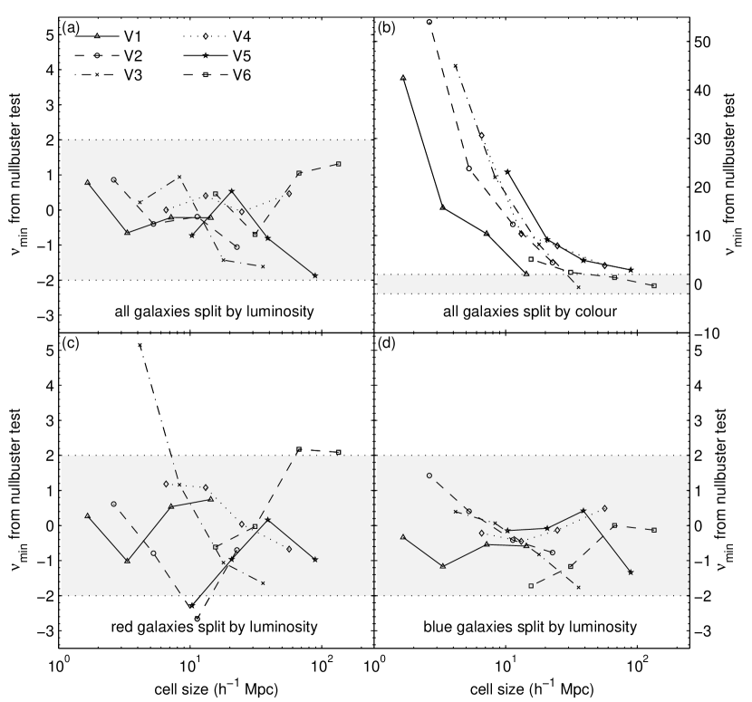
Figure 6: Null-buster results for pairwise comparisons. $\nu_{\mathrm{min}}$ measures the number of sigmas at which deterministic linear biasing can be ruled out as a model of relative bias between the two samples being compared. Shaded areas indicate $\left|\nu_{\mathrm{min}}\right|<2$, where data is consistent with the null hypothesis at the $2\sigma$ level. Four different types of pairwise comparison are illustrated: (a) luminous vs. dim, (b) red vs. blue, (c) luminous red vs. dim red, and (d) luminous blue vs. dim blue. The different symbols denote the different comparison volumes V1-V6. The luminosity-dependent bias (a, c, d) is consistent with deterministic linear biasing but colour-dependent bias (b) is not.

4.1.2 Is the bias independent of scale?

For the luminosity-dependent bias, we use the value of $f$ that gives $\nu_{\mathrm{min}}$ as a measure of $b_{\mathrm{rel}}$, the relative bias between two neighbouring luminosity bins. Since deterministic linear bias is ruled out in the case of the colour-dependent bias, we instead use the value of $b_{\mathrm{rel}}$ from the likelihood analysis here. We find that although the value of $b_{\mathrm{rel}}$ depends on luminosity, it does not appear to depend strongly on scale, as can be seen in Fig. 7: in all plots the curves appear roughly horizontal. To test this ‘chi-by-eye’ inference of scale independence quantitatively, we applied a simple $\chi^{2}$ fit on the four data points (or three in the colour-dependent case) in each volume using a one-parameter model: a horizontal line with a constant value of $b_{\mathrm{rel}}$. For this fit we use covariance matrices derived from jackknife resampling, as discussed in Section B.1. We define this model to be a good fit if the goodness-of-fit value (the probability that a $\chi^{2}$ as poor as as the value calculated should occur by chance, as defined in Press et al. 1992) exceeds 0.01.

We find that this model of no scale dependence is a good fit for all data sets plotted in Fig. 7. We therefore find no evidence that the luminosity- or colour-dependent bias is scale-dependent on the scales we probe here$\left(2-160\,h^{-1}\mathrm{Mpc}\right)$. This implies that recent cosmological parameter analyses which use only measurements on scales $\ga 60{\,h}^{-1}\mathrm{Mpc}$ (e.g., Sánchez et al. 2006; Tegmark et al. 2006; Spergel et al. 2007) are probably justified in assuming scale independence of luminosity-dependent bias.

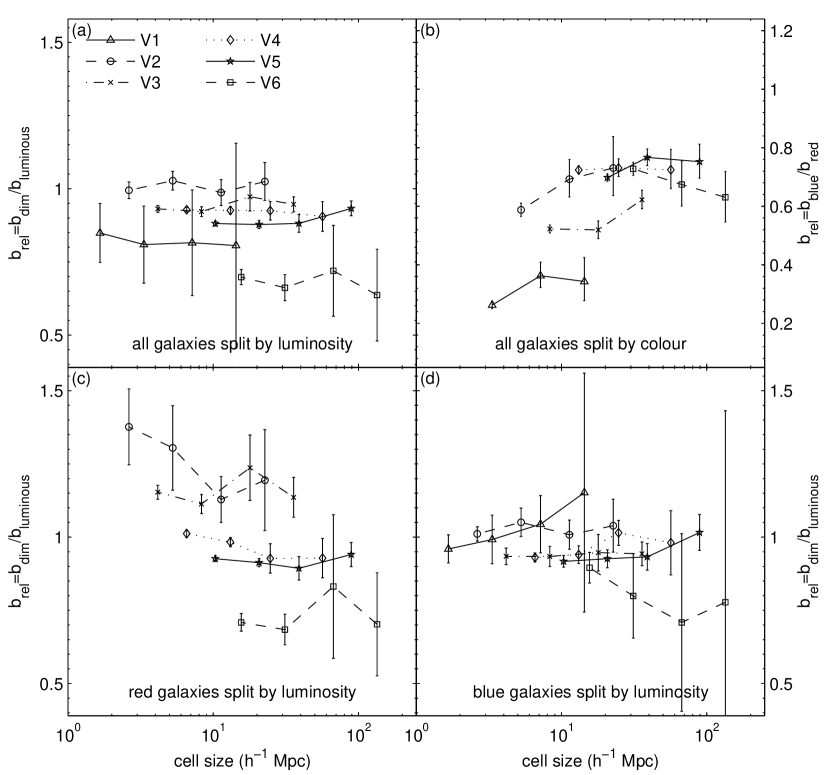
Figure 7: Relative bias $b_{\mathrm{rel}}$ between pairwise samples. (a) luminous vs. dim, (b) red vs. blue, (c) luminous red vs. dim red, and (d) luminous blue vs. dim blue, revealing no significant scale dependence of luminosity- or colour-dependent bias. The $b_{\mathrm{rel}}$ values shown for luminosity dependent splittings (a), (c), and (d) were computed with the null-buster analysis, those shown for the colour-dependent splitting (b) were computed with the likelihood analysis. The different symbols denote the different comparison volumes V1-V6.

In comparison to previous work (Zehavi et al., 2005; Li et al., 2006), it is perhaps surprising to see as little scale dependence as we do – Li et al. (2006) find the luminosity-dependent bias to vary with scale (see their fig. 4), in contrast to what we find here. The measurement of luminosity-dependent bias in Zehavi et al. (2005) agrees more closely with our observation of scale independence, but their their fig. 10 indicates that we might expect to see scale dependence of the luminosity-dependent bias in the most luminous samples. However, we measure the bias in our most luminous samples (in V6) at $16-134\,h^{-1}\mathrm{Mpc}$, well above the range probed in Zehavi et al. (2005), so there is no direct conflict here. Additionally, fig. 13 of Zehavi et al. (2005) and fig. 10 of Li et al. (2006) show that correlation functions of red and blue galaxies have significantly different slopes, implying that the colour-dependent bias should be strongly scale-dependent on $0.1-10\,h^{-1}\mathrm{Mpc}$ scales. However, the points $>1\,h^{-1}\mathrm{Mpc}$ in these plots (the range comparable to the scales we probe here) do not appear strongly scale dependent, so our results are not inconsistent with these correlation function measurements. This interpretation is further supported by recent work (Wang et al., 2007) that finds correlation functions for different luminosities and colours to be roughly parallel above $\sim 1\,h^{-1}\mathrm{Mpc}$.

4.1.3 How bias depends on luminosity

Our next step is to calculate the relative bias parameter $b/b_{*}$ (the bias relative to $L_{*}$ galaxies) as a function of luminosity by combining the measured values of $b_{\mathrm{rel}}$ between the different pairs of luminosity bins. This function has been measured previously using SDSS power spectra (Tegmark et al., 2004b) at length scales of $\sim 60\,h^{-1}\mathrm{Mpc}$ as well as SDSS (Zehavi et al., 2005; Li et al., 2006; Wang et al., 2007) and 2dFGRS (Norberg et al., 2001) correlation functions at length scales of $\sim 1\,h^{-1}\mathrm{Mpc}$ – here we measure it at length scales of $\sim 20\,h^{-1}\mathrm{Mpc}$.

The bias of each luminosity bin relative to the central bin L4 is given by

$$\frac{b_{1}}{b_{4}}=b_{12}b_{23}b_{34},\qquad\frac{b_{2}}{b_{4}}=b_{23}b_{34},\qquad\frac{b_{3}}{b_{4}}=b_{34},$$

$$\frac{b_{7}}{b_{4}}=\frac{1}{b_{45}b_{56}b_{67}},\qquad\frac{b_{6}}{b_{4}}=\frac{1}{b_{45}b_{56}},\qquad\frac{b_{5}}{b_{4}}=\frac{1}{b_{45}},$$ (23)

where $b_{\alpha\beta}$ denotes the measured value of $b_{\mathrm{rel}}$ between luminosity bins L$\alpha$ and L$\beta$ using all galaxies and $b_{\alpha}$ denotes the bias of galaxies in luminosity bin L$\alpha$ relative to the dark matter. For each pairwise comparison, we choose the value of $b_{\mathrm{rel}}$ calculated at the resolution where the cell size is closest to $20\,h^{-1}\mathrm{Mpc}$, as illustrated in Fig. 5. (Since we see no evidence for scale dependence of $b_{\mathrm{rel}}$ for the luminosity-dependent bias, this choice does not strongly influence the results.)

To compute the error bars on $b_{\alpha}/b_{4}$, we rewrite equation (23) as a linear matrix equation using the logs of the bias values:

$$\left(\begin{array}[]{cccccc}1&-1&0&0&0&0\\ 0&1&-1&0&0&0\\ 0&0&1&0&0&0\\ 0&0&0&-1&0&0\\ 0&0&0&1&-1&0\\ 0&0&0&0&1&-1\end{array}\right)\left(\begin{array}[]{c}\log{b_{1}/b_{4}}\\ \log{b_{2}/b_{4}}\\ \log{b_{3}/b_{4}}\\ \log{b_{5}/b_{4}}\\ \log{b_{6}/b_{4}}\\ \log{b_{7}/b_{4}}\end{array}\right)=\left(\begin{array}[]{c}\log{b_{12}}\\ \log{b_{23}}\\ \log{b_{34}}\\ \log{b_{45}}\\ \log{b_{56}}\\ \log{b_{67}}\end{array}\right),$$ (24)

or $\textbf{{A}}{\mn@boldsymbol{b}}_{\mathrm{log}}={\mn@boldsymbol{b}}_{\mathrm{log,rel}}$, where ${\mn@boldsymbol{b}}_{\mathrm{log,rel}}$ is a vector of the log of our relative bias measurements $b_{\alpha\beta}$, ${\mn@boldsymbol{b}}_{\mathrm{log}}$ is a vector of the log of the bias values $b_{\alpha}/b_{4}$, and A is the matrix relating them. We determine the covariance matrix $\mathbf{\Sigma}_{\mathrm{rel}}$ of ${\mn@boldsymbol{b}}_{\mathrm{rel}}$ (a vector of the relative bias measurements $b_{\alpha\beta}$) from the jackknife resampling described in Section B.1, and then compute the covariance matrix $\mathbf{\Sigma}_{\mathrm{log,rel}}$ of ${\mn@boldsymbol{b}}_{\mathrm{log,rel}}$ by

$$\mathbf{\Sigma}_{\mathrm{log,rel}}=\left({\textbf{{B}}}_{\mathrm{rel}}^{T}\right)^{-1}\mathbf{\Sigma}_{\mathrm{rel}}{\textbf{{B}}}_{\mathrm{rel}}^{-1}$$ (25)

where ${\textbf{{B}}}_{\mathrm{rel}}\equiv\mathrm{diag}\left({\mn@boldsymbol{b}}_{\mathrm{rel}}\right)$. We invert equation (24) to give ${\mn@boldsymbol{b}}_{\mathrm{log}}$:

$${\mn@boldsymbol{b}}_{\mathrm{log}}={\textbf{{A}}}^{-1}{\mn@boldsymbol{b}}_{\mathrm{log,rel}},$$ (26)

with the covariance matrix for ${\mn@boldsymbol{b}}_{\mathrm{log}}$ given by

$$\mathbf{\Sigma}_{\mathrm{log}}=\left({\textbf{{A}}}^{T}\mathbf{\Sigma}_{\mathrm{log,rel}}^{-1}\textbf{{A}}\right)^{-1}.$$ (27)

We then fit our data with the model used in Norberg et al. (2001): $b\left(M\right)/b_{*}=a_{1}+a_{2}\left(L/L_{*}\right)$, parameterized by $\mn@boldsymbol{a}\equiv\left(a_{1},\,a_{2}\right)$. Here $M$ is the central absolute magnitude of the bin, $L$ is the corresponding luminosity, and $M_{*}=-20.83$. We use a weighted least-squares fit that is linear in the parameters $\left(a_{1},\,a_{2}\right)$ – that is, we solve the matrix equation

$$\left(\begin{array}[]{c}b_{1}/b_{4}\\ b_{2}/b_{4}\\ b_{3}/b_{4}\\ b_{4}/b_{4}\\ b_{5}/b_{4}\\ b_{6}/b_{4}\end{array}\right)=\left(\begin{array}[]{cc}1&L_{1}/L_{4}\\ 1&L_{2}/L_{4}\\ 1&L_{3}/L_{4}\\ 1&L_{4}/L_{4}\\ 1&L_{5}/L_{4}\\ 1&L_{6}/L_{4}\end{array}\right)\left(\begin{array}[]{c}a_{1}\\ a_{2}\end{array}\right),$$ (28)

or $\mn@boldsymbol{b}=\textbf{{X}}\mn@boldsymbol{a}$, where $\mn@boldsymbol{b}$ is a vector of the bias values $b_{\alpha}/b_{4}$ and X is the matrix representing our model. We solve for $\mn@boldsymbol{a}$ using

$$\mn@boldsymbol{a}=\left({\textbf{{X}}}^{T}\mathbf{\Sigma}^{-1}\textbf{{X}}\right)^{-1}{\textbf{{X}}}^{T}\mathbf{\Sigma}^{-1}\mn@boldsymbol{b}.$$ (29)

Here $\mathbf{\Sigma}$ is the covariance matrix of $\mn@boldsymbol{b}$, given by

$$\mathbf{\Sigma}=\textbf{{B}}\mathbf{\Sigma}_{\mathrm{log}}{\textbf{{B}}}^{T},$$ (30)

where $\mathbf{\Sigma}_{\mathrm{log}}$ is given by equation (27) and $\textbf{{B}}\equiv\mathrm{diag}\left(\mn@boldsymbol{b}\right)$. This procedure gives us the best-fitting values for the parameters $a_{1}$ and $a_{2}$, accounting for the correlations between the data points that are induced we compute the bias values $\mn@boldsymbol{b}$ from our relative bias measurements. We then normalize the model such that $b\left(M_{*}\right)/b_{*}=1$.

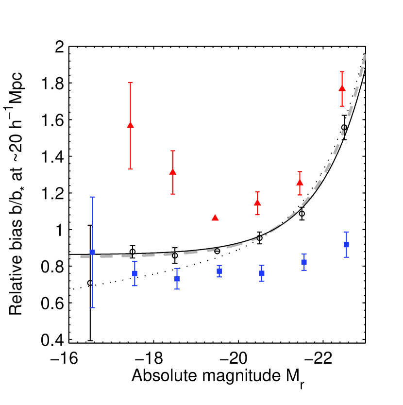
Figure 8: Luminosity dependence of bias for all (open circles), red (solid triangles), and blue (solid squares) galaxies at a cell size of $\sim 20\,h^{-1}\mathrm{Mpc}$ from null-buster results. The solid line is a model fit to the all-galaxy data points, the dotted line shows the model from Tegmark et al. (2004b), and the grey dashed line shows the model from Norberg et al. (2001). The Norberg et al. (2001) model has been computed using the SDSS $r$-band value of $M_{*}=-20.83$.

Figure 8 shows a plot of $b/b_{*}$ vs. $M$: results for all galaxies are plotted with black open circles, our best-fitting model is shown by the solid line, the best-fitting model from Norberg et al. (2001) is shown by the grey dashed line,and the best-fitting model from Tegmark et al. (2004b) is shown by the dotted line. The error bars represent the diagonal elements of $\mathbf{\Sigma}$ from equation (30). Our model, with $\left(a_{1},a_{2}\right)=\left(0.862,\,0.138\right)$, agrees extremely well with the model from Norberg et al. (2001), with $\left(a_{1},a_{2}\right)=\left(0.85,\,0.15\right)$. This agreement is quite remarkable since we use data from a different survey and analyse it with a completely different technique.

A comparison of our results with previous measurements is shown in Fig. 9 in the left panel.

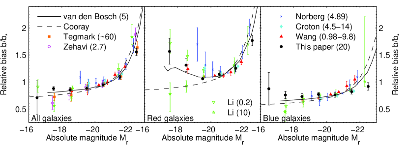
Figure 9: Comparison to previous results for the luminosity dependence of bias for all, red, and blue galaxies. Norberg et al. (2002); Zehavi et al. (2005); Li et al. (2006), and Wang et al. (2007) use correlation function measurements, Tegmark et al. (2004b) use the power spectrum, and Croton et al. (2007) use counts in cells. To better illustrate the similarities and differences in the trends as a function of luminosity, we have normalized all measurements to match our results using the bin closest to $M_{*}=-20.83$. The error bars shown are all relative: they do not include uncertainties due to the normalization. Numbers in parentheses denote the scale in $h^{-1}\mathrm{Mpc}$ at which the measurements were done. Also shown are theoretical models from van den Bosch et al. (2003) (we show their model B as a representative example) and Cooray (2005) – these are also normalized to match our results at $M_{*}$.

In order to compare our SDSS results with results from 2dFGRS (Norberg et al., 2002; Croton et al., 2007), we have added a constant factor of $-1.13$ to their quoted values for $M_{b_{J}}-5\log_{10}h$ in order to line up the value of $M_{*}$ used in Norberg et al. (2002) ($M_{b_{J}}-5\log_{10}h=-19.7$) with the value used here ($M_{{}^{01.}r}=-20.83$). Note that this is necessarily a rough correction since the magnitude in the different bands varies depending on the spectrum of each galaxy, but this method provides a reasonable means of comparing the different results. This plot shows excellent agreement over a wide range of scales, lending further support to our conclusion that the luminosity-dependent bias is independent of scale.

We also use equation (26) to calculate $b/b_{*}$ vs. $M$ for red and blue galaxies separately. To plot the points for red, blue, and all galaxies on the same $b/b_{*}$ vs. $M$ plot, we need to determine their relative normalizations. Applying equation (26) to the red and blue galaxies gives $b_{\alpha,\mathrm{red}}/b_{4,\mathrm{red}}$ and $b_{\alpha,\mathrm{blue}}/b_{4,\mathrm{blue}}$, so to normalize the red-galaxy and blue-galaxy data points to the all-galaxy data points in Fig. 8, we need to calculate

$$\frac{b_{\alpha,\mathrm{red}}}{b_{*,\mathrm{all}}}=\frac{b_{4,\mathrm{all}}}{b_{*,\mathrm{all}}}\frac{b_{4,\mathrm{red}}}{b_{4,\mathrm{all}}}\frac{b_{\alpha,\mathrm{red}}}{b_{4,\mathrm{red}}}$$ (31)

and

$$\frac{b_{\alpha,\mathrm{blue}}}{b_{*,\mathrm{all}}}=\frac{b_{4,\mathrm{all}}}{b_{*,\mathrm{all}}}\frac{b_{4,\mathrm{red}}}{b_{4,\mathrm{all}}}\frac{b_{4,\mathrm{blue}}}{b_{4,\mathrm{red}}}\frac{b_{\alpha,\mathrm{blue}}}{b_{4,\mathrm{blue}}}.$$ (32)

The factor $b_{4,\mathrm{all}}/b_{*,\mathrm{all}}$ is simply the normalization factor chosen for the above model to give $b\left(M_{*}\right)/b_{*}=1$. To determine $b_{4,\mathrm{red}}/b_{4,\mathrm{all}}$, we use best-fitting values of $\sigma_{1}^{2}$ from the likelihood analysis described in Section 3.5 at the resolution with cell sizes closest to $20\,h^{-1}\mathrm{Mpc}$: $\sigma_{1}$ from the comparison of dimmer and more luminous galaxies in V3 gives $b_{4,\mathrm{all}}$, and similarly $\sigma_{1}$ from the comparison of blue and red galaxies in L4 gives $b_{4,\mathrm{red}}$, so

$$\frac{b_{4,\mathrm{red}}}{b_{4,\mathrm{all}}}=\left(\frac{\sigma_{1,\mathrm{red\,vs.\,blue\,L4}}^{2}}{\sigma_{1,\mathrm{lum\,vs.\,dim\,V3}}^{2}}\right)^{1/2}.$$ (33)

The blue points are then normalized relative to the red points using $b_{4,\mathrm{blue}}/b_{4,\mathrm{red}}$ equal to the measured value of $b_{\mathrm{rel}}$ from the likelihood comparison of blue and red galaxies in L4. Thus the shapes of the red and blue curves are determined using the luminosity-dependent bias from the null-buster analysis, but their normalization uses information from the likelihood analysis as well.

Splitting the luminosity dependence of the bias by colour reveals some interesting features. The bias of the blue galaxies shows only a weak dependence on luminosity, and both luminous ($M\sim-22$) and dim ($M\sim-17$) red galaxies have slightly higher bias than moderately bright ($M\sim-20\sim M_{*}$) red galaxies. The previously observed luminosity dependence of bias, with a weak dependence dimmer than $L_{*}$ and a strong increase above $L_{*}$, is thus quite sensitive to the colour selection: the lower luminosity bins contain mostly blue galaxies and thus show weak luminosity dependence, whereas the more luminous bins are dominated by red galaxies which drive the observed trend of more luminous galaxies being more strongly biased. It is instructive to compare these results with the mean local overdensity in colour-magnitude space, as in fig. 2 of Blanton et al. (2005a). Although our bias measurements are necessarily much coarser, it can be seen that the bias is strongest where the overdensity is largest, as has been seen previously (Abbas & Sheth, 2006).

Comparisons of our results to other measurements of luminosity-dependent bias for red and blue galaxies are shown in Fig. 9 in the middle and right panels. Indications of the differing trends for red and blue galaxies have been observed in previous work: an early hint of the upturn in the bias for dim red galaxies was seen in Norberg et al. (2002), and recent results (Wang et al., 2007) also indicate higher bias for dim red galaxies at scales $>1\,h^{-1}\mathrm{Mpc}$. However, there is some inconsistency between these results compared to Zehavi et al. (2005) and Li et al. (2006) regarding the dim red galaxies: they find that dim red galaxies exhibit the strongest clustering on scales $<1\,h^{-1}\mathrm{Mpc}$ and luminous red galaxies exhibit the strongest clustering on larger scales, as can be seen from the green points in Fig. 9. This is shown in fig. 14 of Zehavi et al. (2005) and fig. 11 of Li et al. (2006). However, we find the dim red galaxies to have higher bias than $L_{*}$ red galaxies at all the scales we probe ($2-40\,h^{-1}\mathrm{Mpc}$ in this case). This upturn of the bias for dim red galaxies is present in the halo model-based theoretical curves from van den Bosch et al. (2003), although not in the theoretical curves from Cooray (2005). Note also that van den Bosch et al. (2003) use the data from Norberg et al. (2002) to constrain their models so the agreement between the theory and data should be interpreted with some caution.

Recent measurements of higher order clustering statistics (Croton et al., 2007) find the same trends in the clustering strengths of red and blue galaxies, although they indicate that their linear bias measurement (which should be comparable to ours) shows the opposite trends – little luminosity dependence for red galaxies and a slight monotonic increase for blue galaxies. However, their luminosity range is much narrower than ours so the trends are less clear, and placing their data points on Fig. 9 shows that they are in good agreement with our results.

Previous studies (Norberg et al., 2002; Li et al., 2006; Wang et al., 2007) have also reported a somewhat stronger luminosity dependence of blue galaxy clustering than we have measured here. As can be seen in Fig. 9, Norberg et al. (2002) and Wang et al. (2007) measure slightly higher bias for luminous blue galaxies, and (Li et al., 2006) measure slightly lower bias for dim blue galaxies. Although the quantitative disagreement is fairly small, the qualitative trends of the previous studies imply that the bias of blue galaxies increases with luminosity, as opposed to our measurement which indicates a lack of luminosity dependence.

4.2 Likelihood Results

To study the luminosity dependence, colour dependence and stochasticity of bias in more detail, we also apply the maximum likelihood method described in Section 3.5 to all of the same pairs of samples used in the null-buster test. Due to constraints on computing power and memory, we perform these calculations for only three values of the cell size $L$ rather than four, dropping the highest resolution (smallest cell size) shown in Fig. 4. The likelihood analysis makes a few additional assumptions, but provides a valuable cross-check and also a measurement of the parameter $r_{\mathrm{rel}}$ which encodes the stochasticity and non-linearity of the relative bias.

For each pair of samples, the likelihood function given in equation (22) is maximized with respect to the parameters $\sigma_{1}^{2}$, $b_{\mathrm{rel}}$, and $r_{\mathrm{rel}}$ and marginalized over $\sigma_{1}^{2}$ to determine the best-fitting values of $b_{\mathrm{rel}}$ and $r_{\mathrm{rel}}$, with uncertainties defined by the $\Delta\left(2\ln\mathcal{L}\right)=1$ contour in the $b_{\mathrm{rel}}$-$r_{\mathrm{rel}}$ plane. As we discuss in Section  B.2.3, the values of $b_{\mathrm{rel}}$ found here are consistent with those determined using the null-buster test.

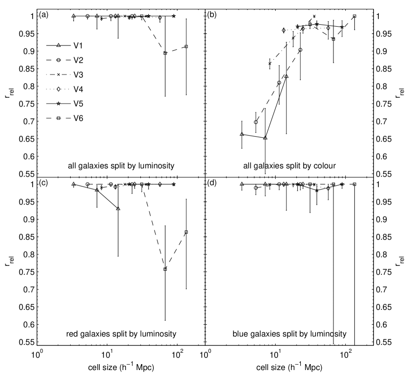
Figure 10: The best-fitting values of the relative cross-correlation coefficient $r_{\mathrm{rel}}$ between pairwise samples. Four different types of pairwise comparison are illustrated: (a) luminous vs. dim, (b) red vs. blue, (c) luminous red vs. dim red, and (d) luminous blue vs. dim blue. The different symbols denote the different comparison volumes V1-V6.

Figure 10 shows the best-fitting values of $r_{\mathrm{rel}}$ as a function of cell size $L$. For the comparisons between neighbouring luminosity bins, the results are consistent with $r_{\mathrm{rel}}=1$. On the other hand, the comparisons between red and blue galaxies give $r_{\mathrm{rel}}<1$, with smaller cell sizes $L$ giving smaller values of $r_{\mathrm{rel}}$. This confirms the null-buster result that the luminosity-dependent bias can be accurately modelled using simple deterministic linear bias but colour-dependent bias demands a more complicated model. Also, $r_{\mathrm{rel}}$ for the colour-dependent bias is seen to depend on scale but not strongly on luminosity. In contrast, $b_{\mathrm{rel}}$ (both in the null-buster and likelihood analyses) depends on luminosity but not on scale.

To summarize, we find that the simple, deterministic model is a good fit for the luminosity-dependent bias, but the colour-dependent bias shows evidence for stochasticity and/or non-linearity which increases in strength towards smaller scales. These results are consistent with previous detections of stochasticity/non-linearity in spectral-type-dependent bias (Tegmark & Bromley, 1999; Blanton, 2000; Conway et al., 2005), and also agree with (Wild et al., 2005) which measures significant stochasticity between galaxies of different colour or spectral type, but not between galaxies of different luminosities.

We compare our results for $r_{\mathrm{rel}}$ for red and blue galaxies to previous results in Fig. 11. This shows good agreement between our results and those of Wild et al. (2005) ($r_{\mathrm{lin}}$ from their fig. 11), implying that these results are quite robust since our analysis uses a different data set, employs different methods, and makes different assumptions.

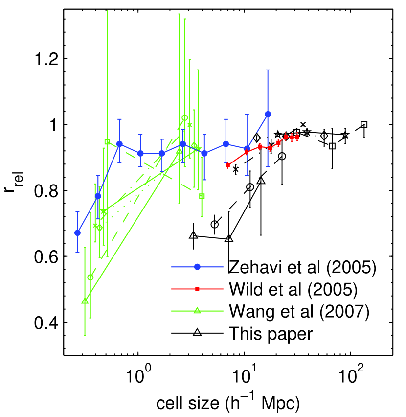
Figure 11: Comparison of relative cross-correlation coefficient $r_{\mathrm{rel}}$ between red and blue galaxies as measured with different techniques. The points from Zehavi et al. (2005) are extracted from cross-correlation measurements between red and blue galaxies in SDSS with $M_{{}^{0.1}r}<-21$, and the Wild et al. (2005) points are from a counts-in-cells analysis using all 2dFGRS galaxies. Our results and the Wang et al. (2007) results (also from SDSS) are separated by luminosity – symbols are the same as in Fig. 10, and for the Wang et al. (2007) results, open triangles denote their dimmest bin ($-19<M_{{}^{01.}r}<-18$) and open squares denote their most luminous bin ($-23<M_{{}^{01.}r}<-21.5$). The length scales used in Wang et al. (2007) are averages over small scales ($0.16-0.98\,h^{-1}\mathrm{Mpc}$) and large scales ($0.98-9.8\,h^{-1}\mathrm{Mpc}$) – points here are shown in the middle of these ranges and offset for clarity.

For the results from cross-correlation measurements, however, the agreement is not as clear. Zehavi et al. (2005) find that the cross-correlation between red and blue galaxies (their fig. 24), indicates that $r_{\mathrm{rel}}$ is consistent with 1 on scales $>1\,h^{-1}\mathrm{Mpc}$. However, it is not clear that this result disagrees with ours, as their result is for luminous galaxies ($M_{{}^{0.1}r}<-21$) and and we do not see a strong indication of $r_{\mathrm{rel}}<1$ for our V6 sample ($23<M_{{}^{0.1}r}<-21$).

More recent cross-correlation measurements (Wang et al., 2007) do find evidence for stochasticity/non-linearity between red and blue galaxies at scales $<1\,h^{-1}\mathrm{Mpc}$ and also show an indication that dimmer galaxies have slightly lower values of $r_{\mathrm{rel}}$. Note also that the method of calculating $r_{\mathrm{rel}}$ by taking ratios of cross- and auto-correlation functions as used for Zehavi et al. (2005) and Wang et al. (2007) does not automatically incorporate the constraint that $\left|r_{\mathrm{rel}}\right|\leq 1$ as our analysis does, so their error bars are allowed to extend above $r_{\mathrm{rel}}=1$ in Fig. 11.

Overall, the counts-in-cells measurements (this paper, Wild et al. 2005) show stronger evidence for stochasticity/non-linearity at larger scales than the cross-correlation measurements (Zehavi et al., 2005; Wang et al., 2007), indicating either that there might be some slight systematic variation between the two methods or that the counts-in-cells method is more sensitive to these effects.

5 Conclusions

To shed further light on how galaxies trace matter, we have quantified how different types of galaxies trace each other. We have analysed the relative bias between pairs of volume-limited galaxy samples of different luminosities and colours using counts-in-cells at varying length scales. This method is most sensitive to length scales between those probed by correlation function and power spectrum methods, and makes point-by-point comparisons of the density fields rather than using ratios of moments, thereby eliminating sample variance and obtaining a local rather than global measure of the bias. We applied a null-buster test on each pair of subsamples to determine if the relative bias was consistent with deterministic linear biasing, and we also performed a maximum-likelihood analysis to find the best-fitting parameters for a simple stochastic biasing model.

5.1 Biasing results

Our primary results are:

1. The luminosity-dependent bias for red galaxies is significantly different from that of blue galaxies: the bias of blue galaxies shows only a weak dependence on luminosity, whereas both luminous and dim red galaxies have higher bias than moderately bright ($L_{*}$) red galaxies.

2. Both of our analysis methods indicate that the simple, deterministic model is a good fit for the luminosity-dependent bias, but that the colour-dependent bias is more complicated, showing strong evidence for stochasticity and/or non-linearity on scales $\la 10h^{-1}$ Mpc.

3. The luminosity-dependent bias is consistent with being scale-independent over the range of scales probed here $\left(2-160\,h^{-1}\mathrm{Mpc}\right)$. The colour-dependent bias depends on luminosity but not on scale, while the cross-correlation coefficient $r_{\mathrm{rel}}$ depends on scale but not strongly on luminosity, giving smaller $r_{\mathrm{rel}}$ values at smaller scales.

These results are encouraging from the perspective of using galaxy clustering to measure cosmological parameters: simple scale-independent linear biasing appears to be a good approximation on the $\ga 60{\,h}^{-1}\mathrm{Mpc}$ scales used in many recent cosmological studies (e.g., Sánchez et al. (2006); Tegmark et al. (2006); Spergel et al. (2007)). However, further quantification of small residual effects will be needed to do full justice to the precision of next-generation data sets on the horizon. Moreover, our results regarding colour sensitivity suggest that more detailed bias studies are worthwhile for luminous red galaxies, which have emerged a powerful cosmological probe because of their visibility at large distances and near-optimal number density (Eisenstein et al., 2001, 2005; Tegmark et al., 2006), since colour cuts are involved in their selection.

5.2 Implications for galaxy formation

What can these results tell us about galaxy formation in the context of the halo model? First of all, as discussed in Zehavi et al. (2005), the large bias of the faint red galaxies can be explained by the fact that such galaxies tend to be satellites in high mass haloes, which are more strongly clustered than low mass haloes. Previous studies have found that central galaxies in low-mass haloes are preferentially blue, central galaxies in high mass haloes tend to be red, and that the luminosity of the central galaxy is strongly correlated with the halo mass (Yang et al., 2005; Zheng et al., 2005). Our observed lack of luminosity dependence of the bias for blue galaxies would then be a reflection of the correlation between luminosity and halo mass being weaker for blue galaxies than for red ones. Additional work is needed to study this quantitatively and compare it with theoretical predictions from galaxy formation models.

The detection of stochasticity between red and blue galaxies may imply that red and blue galaxies tend to live in different haloes – a study of galaxy groups in SDSS (Weinmann et al., 2006) recently presented evidence supporting this, but this is at odds with the cross-correlation measurement in Zehavi et al. (2005), which implies that blue and red galaxies are well-mixed within haloes. The fact that the stochasticity is strongest at small scales suggests that this effect is due to the 1-halo term, i.e., arising from pairs of galaxies in the same halo, although some amount of stochasticity persists even for large scales. However, the halo model implications for stochasticity have not been well-studied to date.

In summary, our results on galaxy biasing and future work along these lines should be able to deepen our understanding of both cosmology (by quantifying systematic uncertainties) and galaxy formation.

Appendix A Consistency Checks

A.1 Alternate null-buster analyses

In order to test the robustness of our results against various systematic effects, we have repeated the null-buster analysis with four different modifications: splitting the galaxy samples randomly, offsetting the pixel positions, using galaxy positions without applying the finger-of-god compression algorithm, and ignoring the cosmological correlations between neighbouring cells.

A.1.1 Randomly split samples

The null-buster test assumes that the Poissonian shot noise for each type of galaxy in each pixel is uncorrelated – i.e., that the matrix N in equation (9) is diagonal – and that this shot noise can be approximated as Gaussian. To test the impact of these assumptions on our results, we repeated the null-buster analysis using randomly split galaxy samples rather than splitting by luminosity or colour. For each volume V1-V6, we created two samples by generating a uniformly distributed random number for each galaxy and assigning it to sample 1 for numbers $>0.5$ and sample 2 otherwise.

If the null-buster test is accurate, we expect the pairwise comparison for the randomly split samples to be consistent with deterministic linear bias with $b_{\mathrm{rel}}=1$. The results are shown in Fig. 12 – we find that, indeed, deterministic linear bias is not ruled out, with nearly all of the $\nu_{\mathrm{min}}$ points falling within $\pm 2$. Furthermore, the measured values of $b_{\mathrm{rel}}$ are seen to be consistent with 1. Thus, we detect no systematic effects due to the null-buster assumptions.

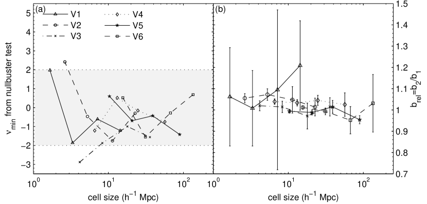
Figure 12: Null-buster results for randomly split samples.

A.1.2 Offset pixel positions

To test if our results are stable against the pixelization chosen, particularly at large scales where we have a small number of cells, we shifted the locations on the sky of the angular pixels defining the cells by half a pixel width in declination. Applying the null-buster analysis to the offset pixels reveals no significant differences from the original analysis: the luminosity-dependent comparisons for all, red, and blue galaxies are still consistent with deterministic linear bias, and the colour-dependent comparison still shows strong evidence for stochasticity and/or nonlinearity, especially at smaller scales.

For the all-, red-, and blue-galaxy, luminosity-dependent comparisons, we also compared the measured values of $b_{\mathrm{rel}}$ from the offset analysis with the original analysis: we took the difference between the two measured values in each volume at each resolution and divided this by the larger of the error bars on the two analyses to determine the number of sigmas by which the two analyses differ. In order to be conservative, we did not add the error bars from the two analyses in quadrature, since this would overestimate the error on the difference if they are correlated and this would make our test less robust. Note that a fully proper treatment would necessitate accounting for the correlations between the errors from each analysis, which we have not done – the discussions in the this and the following sections are meant only to serve as a crude reality check.

For the error bars on the original analysis, we used the jackknife uncertainties described in Section B.1, and for the offset analysis error bars we use the generalized $\chi^{2}$ uncertainties described in Section 3.4 computed from the offset results. (This is because we did not perform jackknife resampling for the offset case or the other modified analyses.)

The results show good agreement: out of a total of 72 measured $b_{\mathrm{rel}}$ values, only 4 differ by more than $2\sigma$ (all galaxies in V3 and V5 at the second-smallest cell size, at $2.6\sigma$ and $3.2\sigma$ respectively, and the red galaxies in V3 and V5 at the second-smallest cell size, at $2.2\sigma$and $3.3\sigma$ respectively). As a rough test for systematic trends, we also counted the number of measurements for which the measured value of $b_{\mathrm{rel}}$ is larger in each analysis. We found that in 38 cases the value from the offset analysis was larger, and in 34 cases the value from the original analysis was larger, indicating no systematic trends in the deviations.

A.1.3 No finger-of-god compression

Our analysis used the finger-of-god compression algorithm from Tegmark et al. (2004b) with a threshold density of $\delta_{c}=200$. This gives a first-order correction for redshift space distortions, but it complicates comparisons to other analyses which work purely in redshift space (e.g. Wild et al. 2005) or use projected correlation functions (e.g. Zehavi et al. 2005), particularly at small scales $\left(\lesssim 10\,h^{-1}\mathrm{Mpc}\right)$ where the effects of virialized galaxy clusters could be significant. To test the sensitivity of our results to this correction, we repeated the null-buster analysis with no finger-of-god compression.

The results show excellent agreement with the original analysis – the smallest-scale measurements for the colour-dependent comparison only rule out deterministic linear bias at 30 sigma rather than 40, but the conclusions remain the same. Additionally, we compared the measured $b_{\mathrm{rel}}$ values to the original analysis as in Section  A.1.2 and find all 72 measurements to be within $2\sigma$. In 25 cases, the analysis without finger-of-god compression gave a larger $b_{\mathrm{rel}}$ value, and in 47 cases the original analysis gave a larger value. This indicates that there might be a very slight tendency to underestimate $b_{\mathrm{rel}}$ if fingers-of-god are not accounted for, but the effect is quite small and well within our error bars. Thus, the finger-of-god compression has no substantial impact on our results.

A.1.4 Uncorrelated signal matrix

The null-buster test requires a choice of residual signal matrix ${\textbf{{S}}}_{\Delta}$ – our analysis uses a signal matrix derived from the matter power spectrum, thus accounting for cosmological correlations between neighbouring cells. However, these correlations are commonly assumed to be negligible in other counts-in-cells analyses (Blanton, 2000; Wild et al., 2005; Conway et al., 2005). To test the sensitivity to the choice of ${\textbf{{S}}}_{\Delta}$, we repeated the analysis using ${\textbf{{S}}}_{\Delta}$ equal to the identity matrix.

Again, we find the results to agree well with the original analysis and lead to the same conclusions. When comparing the measured $b_{\mathrm{rel}}$ values to the original analysis as in Section  A.1.2, we find only 4 out of 72 points differing by more than $2\sigma$ (all galaxies in V5 at the smallest cell size, at $-2.6\sigma$, red galaxies in V4 at the second-smallest and smallest cell size, at $2.2\sigma$ and $2.8\sigma$ respectively, and blue galaxies in V4 at the smallest cell size, at $-3.1\sigma$). In 39 cases the value of $b_{\mathrm{rel}}$ is larger with the uncorrelated signal matrix, and in 33 cases $b_{\mathrm{rel}}$ is larger in the original analysis, indicating no strong systematic effects. Thus we expect our results to be directly comparable to other counts-in-cells analyses done without accounting for cosmological correlations.

Appendix B Uncertainty Calculations

B.1 Jackknife uncertainties for null-buster analysis

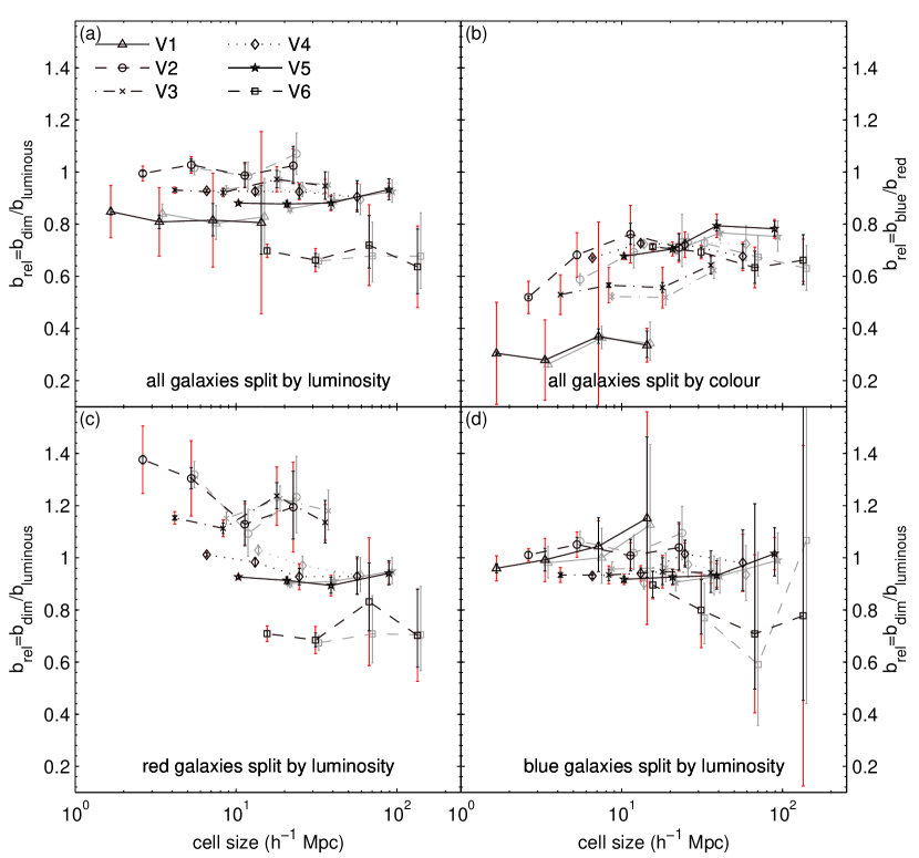
Figure 13: Comparison of two methods for calculating uncertainties on $b_{\mathrm{rel}}$ from the null-buster analysis: jackknife resampling (red) and the generalized $\chi^{2}$ method (black). Also shown are the results for $b_{\mathrm{rel}}$ from the likelihood analysis (grey).

We use jackknife resampling to calculate the uncertainties for the null-buster analysis. The concept is as follows: divide area covered on the sky into $N$ spatially contiguous regions, and then repeat the analysis $N$ times, omitting each of the $N$ regions in turn. The covariance matrix for the measured parameters is then estimated by

$$\mathbf{\Sigma}_{\mathrm{rel}}^{ij}=\frac{N-1}{N}\sum_{k=1}^{N}\left(b_{\mathrm{rel},k}^{i}-\overline{b_{\mathrm{rel}}^{i}}\right)\left(b_{\mathrm{rel},k}^{j}-\overline{b_{\mathrm{rel}}^{j}}\right)$$ (34)

where superscripts $i$ and $j$ denote measurements of $b_{\mathrm{rel}}$ in different volumes and at different scales, $b_{\mathrm{rel},k}^{i}$ denotes the value of $b_{\mathrm{rel}}^{i}$ with the $k$th jackknife region omitted, and $\overline{b_{\mathrm{rel}}^{i}}$ is the average over all $N$ values of $b_{\mathrm{rel},k}^{i}$.

For our analysis, we use the 15 pixels at our lowest resolution (upper left panel in Fig. 4) as the jackknife regions. However, since we use a looser completeness cut at the lowest resolution, two of these pixels cover an area that is not used at higher resolutions. Thus we chose not to include these two pixels in our jackknifes since they do not omit much (or any) area at the higher resolutions. Thus our jackknife resampling has $N=13$. This technique allows us to estimate the uncertainties on all of our $b_{\mathrm{rel}}$ measurements as well as the covariance matrix quantifying the correlations between them. We use these covariances in the model-fitting done in Sections 4.1.2 and 4.1.3.

Figure 13 shows the uncertainties on $b_{\mathrm{rel}}$ as calculated from jackknife resampling compared to those calculated with the generalized $\chi^{2}$ method described in Section 3.4. Overall, the two methods agree well, but the jackknife method gives larger uncertainties at the smallest scales and in volume V1. The reason for the large jackknife uncertainties in volume V1 is because it is significantly smaller than the other volumes, and it is small enough that omitting a cell containing just one large cluster can have a substantial effect on the measured value of $b_{\mathrm{rel}}$. Thus the large uncertainties in V1 reflect the effects of sampling a small volume. Since there are so few dim red galaxies, these effects are particularly egregious for the measurements of luminosity-dependent bias of red galaxies in V1. Thus, based on the jackknife results, we elected to not use V1 in our analysis of the red galaxies.

B.2 Likelihood uncertainties

B.2.1 Likelihood contours

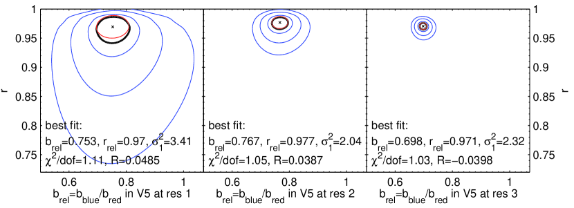
Figure 14: Typical contour plots of $\Delta\left(2\ln\mathcal{L}\right)$ for volume V5 for three different resolutions corresponding (from left- to right-hand-side) to cell sizes of 89, 39, and 21 $h^{-1}\mathrm{Mpc}$. Blue contours denote the $1$, $2$ and $3\sigma$ two-dimensional confidence regions, and black contours denote the $1\sigma$ one-dimensional confidence region used for computing error bars on $b_{\mathrm{rel}}$ and $r_{\mathrm{rel}}$. The red contours denote the error ellipse calculated from the second-order approximation to $2\ln\mathcal{L}$ at the best-fit point, marked with a $\times$.

As described in Section 3.5, we calculate the uncertainty on $b_{\mathrm{rel}}$ and $r_{\mathrm{rel}}$ for the likelihood method using the $\Delta\left(2\ln\mathcal{L}\right)=1$ contour in the $b_{\mathrm{rel}}$-$r_{\mathrm{rel}}$ plane after marginalizing over $\sigma_{1}^{2}$. This means that for each comparison volume and at each resolution, we calculate $\mathcal{L}$ from equation (22) over a grid of $b_{\mathrm{rel}}$ and $r_{\mathrm{rel}}$ values and maximize $2\ln\mathcal{L}$ with respect to $\sigma_{1}^{2}$ at each grid point. This gives us a 2-dimensional likelihood function, which we then maximize to find the best-fit values for $b_{\mathrm{rel}}$ and $r_{\mathrm{rel}}$. Uncertainties are calculated using the function

$$\Delta\left(2\ln\mathcal{L}\left(b_{\mathrm{rel},}r_{\mathrm{rel}}\right)\right)\equiv 2\ln\mathcal{L}\left(b_{\mathrm{rel},}^{\mathrm{max}}r_{\mathrm{rel}}^{\mathrm{max}}\right)-2\ln\mathcal{L}\left(b_{\mathrm{rel},}r_{\mathrm{rel}}\right).$$ (35)

Typical contour plots of this function for volume V5 at each of the three cell sizes used are shown in Fig. 14.

We define 1- and 2-dimensional confidence regions using the standard procedures detailed in Press et al. (1992), using $\Delta\left(2\ln\mathcal{L}\right)$ as an equivalent to $\Delta\chi^{2}$: the $1\sigma$ (68.3%) 1-dimensional confidence region is given by $\Delta\left(2\ln\mathcal{L}\right)=1$, so we define our error bars on $b_{\mathrm{rel}}$ and $r_{\mathrm{rel}}$ by projecting the $\Delta\left(2\ln\mathcal{L}\right)=1$ contour (shown in black in Fig. 14) onto the $b_{\mathrm{rel}}$ and $r_{\mathrm{rel}}$ axes. For illustrative purposes we also show the $1\sigma$, $2\sigma$, and $3\sigma$ (68.3%, 95.4%, and 99.73%) 2-dimensional confidence regions in these plots, given by $\Delta\left(2\ln\mathcal{L}\right)=2.30$, $6.17$, and $11.8$ respectively.

To check the goodness of fit, we also compute an effective value of $\chi^{2}$:

$$\chi_{\mathrm{eff}}^{2}\equiv-2\ln\mathcal{L}-\ln\left|\textbf{{C}}\right|-2n\ln\left(2\pi\right),$$ (36)

where C is given by equation (8) and $n$ is the number of cells. If our model is a good fit, the value of $\chi_{\mathrm{eff}}^{2}$ at the best fit parameter values should be close to the number of degrees of freedom, given by $\mathrm{dof}=2n-2$ ($2n$ data points for type 1 and 2 galaxies in each cell minus 2 parameters $b_{\mathrm{rel}}$ and $r_{\mathrm{rel}}$). We calculated $\chi_{\mathrm{eff}}^{2}/\mathrm{dof}$ for each volume and resolution and found they all lie quite close to 1, ranging from a minimum value of $0.678$ to a maximum value of $1.11$. Thus this test indicates our model is a good fit.

The uncertainties on $b_{\mathrm{rel}}$ and $r_{\mathrm{rel}}$ could perhaps be calculated more accurately using jackknife resampling as we did for the null-buster case; however, repeating the analysis for each jackknife sample is computationally prohibitive since performing all the calculations for just one likelihood analysis took several months of CPU time.

B.2.2 $b_{\mathrm{rel}}$-$r_{\mathrm{rel}}$ covariance matrices

Alternatively, we can calculate the uncertainties using the parameter covariance matrix at the best fit parameter values, as is commonly done in $\chi^{2}$ analyses. The Hessian matrix of second derivatives is given by

$$\textbf{{H}}\equiv\left(\begin{array}[]{cc}\frac{d^{2}\left(2\ln\mathcal{L}\right)}{db_{\mathrm{rel}}^{2}}&\frac{d^{2}\left(2\ln\mathcal{L}\right)}{db_{\mathrm{rel}}dr_{\mathrm{rel}}}\\ \frac{d^{2}\left(2\ln\mathcal{L}\right)}{db_{\mathrm{rel}}dr_{\mathrm{rel}}}&\frac{d^{2}\left(2\ln\mathcal{L}\right)}{dr_{\mathrm{rel}}^{2}}\end{array}\right)$$ (37)

and the parameter covariance matrix is given by

$${\textbf{{C}}}_{\mathrm{param}}\equiv 2{\textbf{{H}}}^{-1}=\left(\begin{array}[]{cc}\sigma_{b_{\mathrm{rel}}}^{2}&\sigma_{{b_{\mathrm{rel}}r}_{\mathrm{rel}}}^{2}\\ \sigma_{{b_{\mathrm{rel}}r}_{\mathrm{rel}}}^{2}&\sigma_{r_{\mathrm{rel}}}^{2}\end{array}\right).$$ (38)

Thus the uncertainties are given by $\sigma_{b_{\mathrm{rel}}}^{2}$ and $\sigma_{r_{\mathrm{rel}}}^{2}$ with this method. This is equivalent to approximating the likelihood function $2\ln\mathcal{L}$ with its second-order Taylor series about the best-fit point, and it defines an error ellipse that approximates the $\Delta\left(2\ln\mathcal{L}\right)=1$ contour. These error ellipses are shown in Fig. 14 in red, and are seen to be in close agreement with the true $\Delta\left(2\ln\mathcal{L}\right)=1$ contours.

This method also allows us to measure the correlation between $b_{\mathrm{rel}}$ and $r_{\mathrm{rel}}$ by calculating the correlation coefficient, given by

$$R\equiv\frac{\sigma_{{b_{\mathrm{rel}}r}_{\mathrm{rel}}}^{2}}{\left(\sigma_{b_{\mathrm{rel}}}^{2}\sigma_{r_{\mathrm{rel}}}^{2}\right)^{1/2}}.$$ (39)

$R$ will fall between -1 (perfectly anti-correlated) and 1 (perfectly correlated). Effectively this measures the tilt of the error ellipse in the $b_{\mathrm{rel}}$-$r_{\mathrm{rel}}$ plane. Overall we find the values of $R$ to be quite small – typically $\left|R\right|\sim 0.05$ – indicating no large correlations between $b_{\mathrm{rel}}$ and $r_{\mathrm{rel}}$. Out of the 72 points we calculate, only 6 have $\left|R\right|>0.3$. The cases with the largest $R$ values are for blue galaxies in volume V6, where the uncertainties are quite large due to the small number of bright blue galaxies and the error ellipses are not good approximations to the likelihood contours anyway – thus these few cases with large $R$ are not overly concerning.

B.2.3 Comparison with null-buster results

Finally, we compare the results for $b_{\mathrm{rel}}$ from the likelihood method to the results from the null-buster analysis in Fig. 13, with the likelihood points shown in grey. As can be seen in this plot, the likelihood and null-buster values for $b_{\mathrm{rel}}$ agree within the uncertainties, even for the colour-dependent bias where the null-buster values are not necessarily accurate since deterministic linear bias is ruled out. Thus our two analysis methods are in excellent agreement with each other.

References

- Abazajian et al. (2005) Abazajian K., Zheng Z., Zehavi I., Weinberg D. H., Frieman J. A., Berlind A. A., Blanton M. R., Bahcall N. A., Brinkmann J., Schneider D. P., Tegmark M., 2005, ApJ, 625, 613
- Abbas & Sheth (2005) Abbas U., Sheth R. K., 2005, MNRAS, 364, 1327
- Abbas & Sheth (2006) Abbas U., Sheth R. K., 2006, MNRAS, 372, 1749
- Adelman-McCarthy et al. (2007) Adelman-McCarthy J. K., et al., 2007, ApJS, 172, 634
- Baldry et al. (2006) Baldry I. K., Balogh M. L., Bower R. G., Glazebrook K., Nichol R. C., Bamford S. P., Budavari T., 2006, MNRAS, 373, 469
- Balogh et al. (2004) Balogh M. L., Baldry I. K., Nichol R., Miller C., Bower R., Glazebrook K., 2004, ApJ, 615, L101
- Baugh (2006) Baugh C. M., 2006, Reports of Progress in Physics, 69, 3101
- Berlind et al. (2005) Berlind A. A., Blanton M. R., Hogg D. W., Weinberg D. H., Davé R., Eisenstein D. J., Katz N., 2005, ApJ, 629, 625
- Berlind & Weinberg (2002) Berlind A. A., Weinberg D. H., 2002, ApJ, 575, 587
- Berlind et al. (2003) Berlind A. A., Weinberg D. H., Benson A. J., Baugh C. M., Cole S., Davé R., Frenk C. S., Jenkins A., Katz N., Lacey C. G., 2003, ApJ, 593, 1
- Blake et al. (2007) Blake C., Collister A., Bridle S., Lahav O., 2007, MNRAS, 374, 1527
- Blanton (2000) Blanton M., 2000, ApJ, 544, 63
- Blanton et al. (003a) Blanton M. R., Brinkmann J., Csabai I., Doi M., Eisenstein D., Fukugita M., Gunn J. E., Hogg D. W., Schlegel D. J., 2003a, AJ, 125, 2348
- Blanton et al. (005a) Blanton M. R., Eisenstein D., Hogg D. W., Schlegel D. J., Brinkmann J., 2005a, ApJ, 629, 143
- Blanton et al. (2006) Blanton M. R., Eisenstein D., Hogg D. W., Zehavi I., 2006, ApJ, 645, 977
- Blanton et al. (003b) Blanton M. R., Lin H., Lupton R. H., Maley F. M., Young N., Zehavi I., Loveday J., 2003b, AJ, 125, 2276
- Blanton et al. (005b) Blanton M. R., Schlegel D. J., Strauss M. A., Brinkmann J., Finkbeiner D., Fukugita M., Gunn J. E., Hogg D. W., Ivezić Ž., Knapp G. R., Lupton R. H., Munn J. A., Schneider D. P., Tegmark M., Zehavi I., 2005b, AJ, 129, 2562
- Broadhurst et al. (1995) Broadhurst T. J., Taylor A. N., Peacock J. A., 1995, ApJ, 438, 49
- Casas-Miranda et al. (2002) Casas-Miranda R., Mo H. J., Sheth R. K., Boerner G., 2002, MNRAS, 333, 730
- Catelan et al. (1998) Catelan P., Lucchin F., Matarrese S., Porciani C., 1998, MNRAS, 297, 692
- Cole et al. (2005) Cole S., et al., 2005, MNRAS, 362, 505
- Colless et al. (2001) Colless M., et al., 2001, MNRAS, 328, 1039
- Collister & Lahav (2005) Collister A. A., Lahav O., 2005, MNRAS, 361, 415
- Conway et al. (2005) Conway E., et al., 2005, MNRAS, 356, 456
- Cooray (2005) Cooray A., 2005, MNRAS, 363, 337
- Cooray (2006) Cooray A., 2006, astro-ph/0601090
- Cooray & Sheth (2002) Cooray A., Sheth R., 2002, Phys. Rep., 372, 1
- Croton et al. (2007) Croton D. J., Norberg P., Gaztañaga E., Baugh C. M., 2007, MNRAS, 379, 1562
- Croton et al. (2006) Croton D. J., Springel V., White S. D. M., De Lucia G., Frenk C. S., Gao L., Jenkins A., Kauffmann G., Navarro J. F., Yoshida N., 2006, MNRAS, 365, 11
- Davis & Geller (1976) Davis M., Geller M. J., 1976, ApJ, 208, 13
- Dekel & Lahav (1999) Dekel A., Lahav O., 1999, ApJ, 520, 24
- Dodelson et al. (1997) Dodelson S., Hui L., Jaffe A., 1997, astro-ph/9712074
- Eisenstein et al. (2001) Eisenstein D. J., et al., 2001, AJ, 122, 2267
- Eisenstein et al. (2005) Eisenstein D. J., et al., 2005, ApJ, 633, 560
- Fukugita et al. (1996) Fukugita M., Ichikawa T., Gunn J. E., Doi M., Shimasaku K., Schneider D. P., 1996, AJ, 111, 1748
- Gao & White (2007) Gao L., White S. D. M., 2007, MNRAS, 377, L5
- Gunn et al. (1998) Gunn J. E., et al., 1998, AJ, 116, 3040
- Gunn et al. (2006) Gunn J. E., et al., 2006, AJ, 131, 2332
- Guzzo et al. (1997) Guzzo L., Strauss M. A., Fisher K. B., Giovanelli R., Haynes M. P., 1997, ApJ, 489, 37
- Hamilton (1988) Hamilton A. J. S., 1988, ApJ, 331, L59
- Hamilton & Tegmark (2004) Hamilton A. J. S., Tegmark M., 2004, MNRAS, 349, 115
- Hogg et al. (2004) Hogg D. W., Blanton M. R., Brinchmann J., Eisenstein D. J., Schlegel D. J., Gunn J. E., McKay T. A., Rix H.-W., Bahcall N. A., Brinkmann J., Meiksin A., 2004, ApJ, 601, L29
- Hogg et al. (2001) Hogg D. W., Finkbeiner D. P., Schlegel D. J., Gunn J. E., 2001, AJ, 122, 2129
- Hubble & Humason (1931) Hubble E., Humason M. L., 1931, ApJ, 74, 43
- Ivezić et al. (2004) Ivezić Ž., et al., 2004, Astronomische Nachrichten, 325, 583
- Joyce et al. (2005) Joyce M., Sylos Labini F., Gabrielli A., Montuori M., Pietronero L., 2005, A&A, 443, 11
- Kravtsov (2006) Kravtsov A. V., 2006, astro-ph/0607463
- Kravtsov et al. (2004) Kravtsov A. V., Berlind A. A., Wechsler R. H., Klypin A. A., Gottlöber S., Allgood B., Primack J. R., 2004, ApJ, 609, 35
- Kristiansen et al. (2007) Kristiansen J. R., Elgarøy Ø., Dahle H., 2007, Phys. Rev. D, 75, 083510
- Li et al. (2006) Li C., Kauffmann G., Jing Y. P., White S. D. M., Börner G., Cheng F. Z., 2006, MNRAS, 368, 21
- Loveday et al. (1995) Loveday J., Maddox S. J., Efstathiou G., Peterson B. A., 1995, ApJ, 442, 457
- Lupton et al. (2001) Lupton R., Gunn J. E., Ivezić Z., Knapp G. R., Kent S., 2001, in Harnden Jr. F. R., Primini F. A., Payne H. E., eds, ASP Conf. Ser. Vol. 238, Astronomical Data Analysis Software and Systems X. Astron. Soc. Pac., San Francisco, pp 269–+
- Madgwick et al. (2003) Madgwick D. S., et al., 2003, MNRAS, 344, 847
- Magliocchetti & Porciani (2003) Magliocchetti M., Porciani C., 2003, MNRAS, 346, 186
- Mateus et al. (2006) Mateus A., Sodré L., Cid Fernandes R., Stasińska G., Schoenell W., Gomes J. M., 2006, MNRAS, 370, 721
- Matsubara (1999) Matsubara T., 1999, ApJ, 525, 543
- McDonald (2006) McDonald P., 2006, Phys. Rev. D, 74, 103512
- Möller et al. (2007) Möller O., Kitzbichler M., Natarajan P., 2007, MNRAS, 379, 1195
- Norberg et al. (2001) Norberg P., et al., 2001, MNRAS, 328, 64
- Norberg et al. (2002) Norberg P., et al., 2002, MNRAS, 332, 827
- Novosyadlyj et al. (1999) Novosyadlyj B., Durrer R., Lukash V. N., 1999, A&A, 347, 799
- Padmanabhan et al. (2007) Padmanabhan N., et al., 2007, MNRAS, 378, 852
- Park et al. (1994) Park C., Vogeley M. S., Geller M. J., Huchra J. P., 1994, ApJ, 431, 569
- Peacock (1999) Peacock J. A., 1999, Cosmological Physics. Cosmological Physics, by John A. Peacock, pp. 704. ISBN 052141072X. Cambridge, UK: Cambridge University Press, January 1999.
- Peacock & Smith (2000) Peacock J. A., Smith R. E., 2000, MNRAS, 318, 1144
- Pen (1998) Pen U.-L., 1998, ApJ, 504, 601
- Percival et al. (2007) Percival W. J., Nichol R. C., Eisenstein D. J., Frieman J. A., Fukugita M., Loveday J., Pope A. C., Schneider D. P., Szalay A. S., Tegmark M., Vogeley M. S., Weinberg D. H., Zehavi I., Bahcall N. A., Brinkmann J., Connolly A. J., Meiksin A., 2007, ApJ, 657, 645
- Percival et al. (2004) Percival W. J., Verde L., Peacock J. A., 2004, MNRAS, 347, 645
- Pier et al. (2003) Pier J. R., Munn J. A., Hindsley R. B., Hennessy G. S., Kent S. M., Lupton R. H., Ivezić Ž., 2003, AJ, 125, 1559
- Press et al. (1992) Press W. H., Teukolsky S. A., Vetterling W. T., Flannery B. P., 1992, Numerical recipes in C. The art of scientific computing. Cambridge: University Press, —c1992, 2nd ed.
- Sánchez et al. (2006) Sánchez A. G., Baugh C. M., Percival W. J., Peacock J. A., Padilla N. D., Cole S., Frenk C. S., Norberg P., 2006, MNRAS, 366, 189
- Schechter (1976) Schechter P., 1976, ApJ, 203, 297
- Schlegel et al. (1998) Schlegel D. J., Finkbeiner D. P., Davis M., 1998, ApJ, 500, 525
- Scranton (2003) Scranton R., 2003, MNRAS, 339, 410
- Sefusatti & Scoccimarro (2005) Sefusatti E., Scoccimarro R., 2005, Phys. Rev. D, 71, 063001
- Seljak (2000) Seljak U., 2000, MNRAS, 318, 203
- Seljak (2001) Seljak U., 2001, MNRAS, 325, 1359
- Seljak et al. (2005) Seljak U., Makarov A., Mandelbaum R., Hirata C. M., Padmanabhan N., McDonald P., Blanton M. R., Tegmark M., Bahcall N. A., Brinkmann J., 2005, Phys. Rev. D, 71, 043511
- Seljak & Warren (2004) Seljak U., Warren M. S., 2004, MNRAS, 355, 129
- Sheth et al. (2005) Sheth R. K., Connolly A. J., Skibba R., 2005, astro-ph/0511773
- Sheth & Diaferio (2001) Sheth R. K., Diaferio A., 2001, MNRAS, 322, 901
- Simon (2005) Simon P., 2005, A&A, 430, 827
- Simon et al. (2007) Simon P., Hetterscheidt M., Schirmer M., Erben T., Schneider P., Wolf C., Meisenheimer K., 2007, A&A, 461, 861
- Skibba et al. (2006) Skibba R., Sheth R. K., Connolly A. J., Scranton R., 2006, MNRAS, 369, 68
- Smith et al. (2002) Smith J. A., et al., 2002, AJ, 123, 2121
- Smith et al. (2003) Smith R. E., Peacock J. A., Jenkins A., White S. D. M., Frenk C. S., Pearce F. R., Thomas P. A., Efstathiou G., Couchman H. M. P., 2003, MNRAS, 341, 1311
- Smith et al. (2007) Smith R. E., Scoccimarro R., Sheth R. K., 2007, Phys. Rev. D, 75, 063512
- Somerville et al. (2001) Somerville R. S., Lemson G., Sigad Y., Dekel A., Kauffmann G., White S. D. M., 2001, MNRAS, 320, 289
- Spergel et al. (2007) Spergel D. N., et al., 2007, ApJS, 170, 377
- Stoughton et al. (2002) Stoughton C., et al., 2002, AJ, 123, 485
- Swanson et al. (2007) Swanson M. E. C., Tegmark M., Hamilton A. J. S., Hill J. C., 2007, arXiv:0711.4352
- Tegmark (1999) Tegmark M., 1999, ApJ, 519, 513
- Tegmark & Bromley (1999) Tegmark M., Bromley B. C., 1999, ApJ, 518, L69
- Tegmark et al. (2004a) Tegmark M., et al., 2004a, Phys. Rev. D, 69, 103501
- Tegmark et al. (2004b) Tegmark M., et al., 2004b, ApJ, 606, 702
- Tegmark et al. (2006) Tegmark M., et al., 2006, Phys. Rev. D, 74, 123507
- Tegmark & Peebles (1998) Tegmark M., Peebles P. J. E., 1998, ApJ, 500, L79+
- Tinker et al. (2007) Tinker J. L., Norberg P., Weinberg D. H., Warren M. S., 2007, ApJ, 659, 877
- Tinker et al. (2006) Tinker J. L., Weinberg D. H., Warren M. S., 2006, ApJ, 647, 737
- Tucker et al. (2006) Tucker D. L., et al., 2006, Astronomische Nachrichten, 327, 821
- Uomoto et al. (2004) Uomoto A., Smee S. A., Barkhouser R. H., 2004, in Moorwood A. F. M., Iye M., eds, Proc. SPIE Vol. 5492, Ground-based Instrumentation for Astronomy. Int. Soc. Opt. Eng., Bellingham, WA, pp 1411–1422
- van den Bosch et al. (2003) van den Bosch F. C., Yang X., Mo H. J., 2003, MNRAS, 340, 771
- Wang et al. (2007) Wang Y., Yang X., Mo H. J., van den Bosch F. C., 2007, ApJ, 664, 608
- Weinmann et al. (2006) Weinmann S. M., van den Bosch F. C., Yang X., Mo H. J., 2006, MNRAS, 366, 2
- White et al. (1988) White S. D. M., Tully R. B., Davis M., 1988, ApJ, 333, L45
- Wild et al. (2005) Wild V., et al., 2005, MNRAS, 356, 247
- Willmer et al. (1998) Willmer C. N. A., da Costa L. N., Pellegrini P. S., 1998, AJ, 115, 869
- Yang et al. (2005) Yang X., Mo H. J., Jing Y. P., van den Bosch F. C., 2005, MNRAS, 358, 217
- Yang et al. (2003) Yang X., Mo H. J., van den Bosch F. C., 2003, MNRAS, 339, 1057
- Yang et al. (2006) Yang X., Mo H. J., van den Bosch F. C., 2006, ApJ, 638, L55
- York et al. (2000) York D. G., et al., 2000, AJ, 120, 1579
- Zehavi et al. (2005) Zehavi I., et al., 2005, ApJ, 630, 1
- Zheng et al. (2005) Zheng Z., Berlind A. A., Weinberg D. H., Benson A. J., Baugh C. M., Cole S., Davé R., Frenk C. S., Katz N., Lacey C. G., 2005, ApJ, 633, 791
- Zheng & Weinberg (2007) Zheng Z., Weinberg D. H., 2007, ApJ, 659, 1