Strong lensing, dark matter and $H_{0}$ estimate

Abstract

Gravitational lensing represents a powerful tool to estimate the cosmological parameters and the distribution of dark matter. I will describe the main observable quantities, concentrating on strong lensing, that manifests its effect through the formation of spectacular events, like multiple quasars, Einstein rings and arcs in clusters of galaxies. In events where a quasar is lensed by an intervening galaxy, it is possible to give an estimate of the Hubble constant $H_{0}$, by choosing a mass density model for the lens, thus allowing to constrain the dark matter content.

1 Introduction: historical remarks

Gravitational lensing (GL), born as a theoretical prediction, has became a powerful tool to explore the universe. It concerns all those phenomena linked to the deflection of light of faraway sources due to the presence of an intervening astrophysical body, named ‘lens’. The concept of light deflection is also present in the Newtonian physics: in fact during 1700-1800 some scientists, like Newton, Cavendish and Soldner studied this problem giving an estimate of this deflection.

In the beginning of the last century, Einstein elaborated its revolutionary theory of General Relativity, allowing him to give the correct prediction for the deflection angle of a point mass lens, given by

$$\hat{\alpha}=\frac{4GM}{c^{2}\,r},$$ (1)

where $M$ is the mass of lens and $r$ is the distance at which the ray passes near the lens. Eq. (1) is twice of the classical prediction. Observing the change in the position of stars on the limb of the sun during an eclipse in 1919, Sir A. Eddington was able to verify the prediction of Einstein, thus providing the first experimental proof of General Relativity .

In 1934 Zwicky was the first to consider that also galaxies would be able to act as lenses, increasing the possibility of observing these phenomena also on larger scales. In 1964 Refsdal analyzed the possibility to use GL as a tool to study cosmological parameters and in particular to estimate Hubble constant.

In 1979 Walsh, Carswell e Weymann [1] observed the first lens, a couple of nearby and very similar quasars, images of the same source, the double quasar Q 0957+561. In the next two decades other events were observed: many other multiple lensed quasars, arcs and arclets in clusters of galaxies, Einstein rings, extragalactic and galactic microlensing, weak lensing, etc. etc. [1]

2 Basics of gravitational lensing

GL takes place when a lens (a star, a galaxy or a cluster of galaxies) crosses (or is near to) the line of sight to a distant source. Under the “weak field approximation”, the lens only perturbs “little” the space-time metric, which can be written as [1, 2, 3]

$$ds^{2}=\bigg{(}1+\frac{2U}{c^{2}}\bigg{)}dt^{2}-\bigg{(}1-\frac{2U}{c^{2}}\bigg{)}d\textbf{x}^{2}$$ (2)

where $(t,\textbf{x})$ are time and 3-D space coordinates, and $U(\textbf{x})$ the gravitational potential. We exclude “strong fields”, like those generated by black hole and neutron stars, that need more a complex analysis.

We can distinguish three regimes

• strong lensing that consists in the formation of multiple (magnified) images of the source (lensed quasars, Einstein rings and arcs in clusters of galaxies),

• microlensing as a case of strong lensing, when the images are blended and undistinguishable (extragalactic and galactic microlensing),

• weak lensing characterized only by a deformation and a light amplification of the images without formation of different images; this regime is practically present in every astronomical image.

We will analyze the first regime, mainly describing the observables that characterize it and concentrating on the spectacular events it can generate. We can identify three main observable phenomena:

1. formation of images,

2. (de)amplification of images,

3. time delay among the images.

2.1 Deflection angle and lens equation

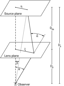
The prediction of Einstein regarded the deflection angle of a star of mass $M$. In more general situations, when the lens is a galaxy or a cluster of galaxies, this expression is more complex: the deflection will depend on the mass distribution of the lens. Weak field approximation allows us to use Eq. (2) and to manage small angle [1] (in common situations, the angular separations of the images is $<30^{\prime\prime}$). Therefore, we can analyze a lensed events in a thin cone around the line of sight observer-lens, studying the phenomena in two plane builded on the lens (lens plane) and source (source plane). In addition, the lens can be considered “thin” (since the extension along the line of sight is small respect to the transversal dimensions), and therefore all we need to know are the quantities projected on the lens plane, first of all the surface mass density of the lens $\Sigma(\xi)$ (see, for instance, Fig. 1).

Figure 1: Typical lens configuration of a lensing events. We observe the lens and source planes. The long dashed line represents the line of sight observer-lens, the vector $\vec{\eta}$ (and the corresponding angle $\vec{\beta}$) specifies the position of the source on the relative plane, and the vector $\vec{\xi}$ (and the relative angle $\vec{\theta}$) the position of the generic images on the lens plane. Crucial ingredients in such a configuration are the distances, $D_{s}$, $D_{d}$ and $D_{ds}$. In cosmological applications, angular diameter distances are used, depending on the redshift $z$ of the considered object and on the cosmological model parameters.

For a generic surface mass density $\Sigma(\vec{\xi})$, the lensing angle is given by

$$\vec{\hat{\alpha}}(\vec{\xi})\equiv\frac{4G}{c^{2}}{\int}\frac{\vec{\xi}-\vec{\xi}^{\prime}}{{|\vec{\xi}-\vec{\xi}^{\prime}|}^{2}}\Sigma(\vec{\xi}^{\prime})d^{2}\xi^{\prime},$$ (3)

We can derive a two dimensional relation between the positions of images and source, the so called lens equation or lens mapping

$$\vec{\beta}=\vec{\theta}-\vec{\alpha}(\vec{\theta})$$ (4)

where $\vec{\alpha}(\theta)=\frac{D_{ds}}{D_{s}}\vec{\hat{\alpha}}(\theta)$ is the adimensional lensing angle. Given the source position angle $\vec{\beta}$, Eq. (4) is a non linear equation of the image position angle $\vec{\theta}$, thus a generic lens distribution generates more than 1 image.

2.2 Lensing magnification

A lens also acts as a sort of a telescope, magnifying the sources. In addition to a deformation of the path of a light ray, the lens modifies the transversal section of a light bundle, enlarging or reducing its sectional area and changing its form. The lens does not affect light intensity, and thus the amplification of an image only depends on the angles subtended by the image itself and source.

2.3 Time delay

The images of a lensed source are characterized by a time delay, i.e. in one of the images the lensed object will be observed before than the other ones. The time delay between a generic path from source to observer and the unlensed ray is given by [1, 2, 3]

$$\Delta t(\vec{\beta},\vec{\theta})=\frac{1+z_{d}}{c}\frac{D_{d}D_{s}}{D_{ds}}\bigg{(}\frac{1}{2}(\vec{\theta}-\vec{\beta})^{2}-\psi(\vec{\theta})\bigg{)},$$ (5)

where $z_{d}$ is the lens redshift and $\psi$ is the so called lensing potential, linked to the adimensional lensing angle $\vec{\alpha}$ by means of the gradient $\vec{\alpha}=\vec{\nabla}_{\theta}\psi$. It is clear the contribution of two effects: a geometric term, due to the different paths traveled respect to the unlensed straight line from the source to the observer, a gravitational one, due to the effect of gravitational potential of the lensing mass.

If the source has a luminosity variable with the time (this is the case of some quasars), different features in the light curve can be revealed delayed in the different images and the relative time lag can be measured. Thus, while $\Delta t$ is not measurable, since we do not see the unlensed source, it is possible to measure the quantity

$$\Delta t_{ij}=\Delta t(\vec{\beta},\vec{\theta}_{j})-\Delta t(\vec{\beta},\vec{\theta}_{i}),$$ (6)

i.e., the time delay between the $j^{th}$ and $i^{th}$ images in a lensing event.

Figure 2: Image configurations in quadruply lensed events. For the double quasars are possible two configurations that we do not report here.

2.4 Some details about image formation

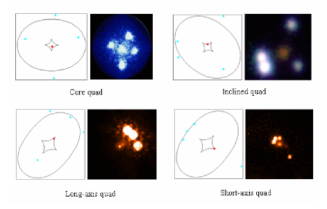
It is possible to classify the images in a simple way. We distinguish two kinds of images: ordinary and critical ones. Ordinary images occur at the points where the lens equation is verified and where the amplification is finite. On the contrary, for some critical points the lens mapping is not invertible and the amplification is infinite. These points form on the lens plane closed curves, named critical curves, and if we map them to the source plane we get other closed curves, named caustics. We can distinguish two kinds of critical curves: radial and tangential ones, but the second ones are crucial in our case to analyze the formation of images. Limiting the attention to the case of a single lens: for spherical mass distribution the critical curves are circular, the tangential caustic is point-like and the radial one is circular, in this case, in addition to a central image, two images form; for elliptical mass distribution the critical curves are not circular, the tangential caustic becomes an astroid with folds and cuspids (see Fig. 2) and in addition to an eventual central image, we can have 2 or 4 images.

In particular, when a source approaches the astroid from the inner side, two images fuse and disappear, thus passing from a 4-images to a 2-images configuration. In typical lensing events, when the source is near a fold, we observe two nearby images, one on a side of the critical curves and another to the other side (see inclined quad in Fig. 2), on the contrary, when the source is near a cusp, 3 images form near the critical curves (see lower panels in Fig. 2). These images are magnified respect to the other ones, as can be easily verified in real cases by an inspections of the quasars in Fig. 2. More complex configurations with a higher number of images are possible when more than one lens are considered.

3 Ingredients to shape lensed quasars

In order to analyze a lensing event, we need to know some information about lens galaxy and quasar. We need the image positions respect to the primary lens galaxy, the flux ratios and time delays, the lens and source redshift $z_{d}$ and $z_{s}$ and in addition other information about the galaxy (like the luminous profile, the velocity dispersion profile, etc.). The quantities to be estimated are source position, the cosmological parameters (density parameters and $H_{0}$) and the lens model [1, 2].

Time delay in Eq. (5) can assume the factorized expression

$$\Delta t_{ij}=\frac{1}{H_{0}}T(\textrm{distances},z_{d},z_{s})f(\textrm{lens model},\theta_{i},\theta_{j},z_{d},z_{s})$$ (7)

where $T$ contains the contribution of the cosmology ($T\to 0$ when is $z_{i}\to 0$ or we consider an Euclidean universe) and $f$ crucially depends on the lens model. The function $T$ is fixed assuming some fiducial values for the cosmological parameters, $H_{0}$ and the lens model remain to be fitted. In many cases (if we use standard models of Universe), the uncertainties introduced by fixing the function $T$ amounts to some percentages. Therefore, using the constraints above (comprising the time delays), we have to choice a form for the lens model and fit it to these observables.

4 Lens model

When possible (i.e., when along the line of sight we observe a single galaxy, with other objects enough faraway from it) we have to choose a form for the potential of the primary lens and shape the contribution of other galaxies or external groups of galaxies with an external shear.

The main galaxy needs a full modeling with the choice of a particular galaxy model. We can distinguish two classes of models, linked to the kind of matter we are considering, luminous or dark matter

• Luminous matter. The stars in galaxy emit a lot of luminous radiation. Thus, one measures the light profile of galaxy as a function of the radius from its center. The most credited models are the de Vaucouleurs law, or other profiles from Hernquist, Jaffe, Dehnen, Hubble, etc. In order to obtain the mass profile we use the assumption of a constant M/L ratio, reasonable since in this case all the matter exists is observed by its emitted light.

• Dark matter. Galaxies and cluster of galaxies seem to be filled by a huge quantity of an unseen matter (dark matter). Different approaches can be chosen to describe dark matter profiles, starting from theoretical models (singular isothermal sphere, models starting from distribution function, etc.), models from simulations (NFW model) or empirical analysis (Sersic model).

The external perturbations is taken into account by means of the so called shear, developing $\psi$ to the $2^{nd}$ order

$$\psi_{\gamma}(r,\theta)=-\frac{1}{2}\gamma\ r^{2}\cos 2(\theta-\theta_{\gamma}),$$ (8)

where $\gamma$ is the shear amplitude and $\theta_{\gamma}$ fixes the direction where is the perturbation.

5 Estimate of Hubble constant

$H_{0}$ is a main parameter in cosmology, crucially influencing the dynamics of the universe. GL is a tool to estimate cosmological parameters and particularly $H_{0}$, complementary to other methods like cosmic distance ladder, anisotropy of the cosmic microwave background radiation, the Sunyaev-Zel’dovich effect, etc.

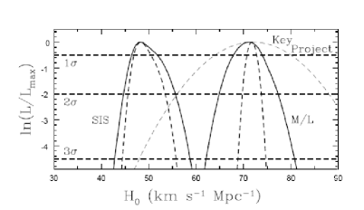
GL has many advantages respect to other methods, allowing to avoid, for example, the propagation of the uncertainties we can observe in the application of the cosmic distance ladder, but the choice of lens model remains a huge source of uncertainty. Two results discussed in literature concern the fact that the same lens configuration is well reproduced by different classes of models, and the corresponding dependence of estimated $H_{0}$ from the chosen lens model. In particular, constant $M/L$ profiles systematically furnish higher values of $H_{0}$ than those given by profiles with dark matter (like, in the simplest case, the SIS). See Fig. 3, where we see the estimated value from HST Key project is not consistent within $2\sigma$ with the lensing estimate using a SIS profile, but in agreement with the estimates using constant M/L profiles [2].

Figure 3: Joint $H_{0}$ likelihood distribution using 4 lenses and assuming a SIS (left curves) and a constant $M/L$ model (right curves) and the results from HST Key project (light dashed curves).

We verified this result, using more complex dark matter models and two different constant $M/L$ profiles [4]. The first models are fixed by choosing a simple separable form for the lensing potential

$$\psi(r,\theta)=F(\theta,q,\theta_{q})r^{\alpha},$$ (9)

where the function $F$ specifies the angular dependence, $(q,\theta_{q})$ are the the axial ratio and the angle of the orientation of lensing potential, and $\alpha$ is a slope parameter. The constant M/L models are the de Vaucouleurs and Hubble profiles. The degeneracy and the interesting results above are evident in our work, also being our estimates affected by huge uncertainties due to our method and the degeneracies existing among the lens parameters and $H_{0}$ itself. Finally, marginalizing over the results from different models and over two different lensed quasars we obtain

$$H_{0}=56\pm 23\textrm{ km}\ \textrm{s}^{-1}\ \textrm{Mpc}^{-1}$$ (10)

Using the model in Eq. (9), leaving the function F unspecified and suitably manipulating the lens and time delay equations, it is possible to model at the same time different lensed events that share the same $H_{0}$. Thus, we can obtain an estimate of $H_{0}$ modeling different lensed quasars all at once. Using 2 lensed quasars, the results is [4]

$$H_{0}=49^{+6}_{-11}\textrm{ km}\ \textrm{s}^{-1}\ \textrm{Mpc}^{-1}$$ (11)

6 A general choice for the lens model

As remarked above, the choice of lens model remains the main source of uncertainties in the estimate of $H_{0}$ by means of lensed quasars. Since we do not know what is the ‘right’ profile of galaxy, we can follow two different routes.

The first one was previously discussed and consists to do a marginalization over different models in order to obtain an estimate of $H_{0}$ not depending on the particular choice of model, but in some sense weighing the single estimates obtained using each model with its uncertainty.

The second one consists to assume a very general form for the lens model, able to reproduce different behaviors, spanning from $M/L$ profile (with declining rotation curves) to dark matter profile (with flat rotation curves). We start from this general requirement and thus choose a double power law expression for the $M/L$ ratio [5]

$$\Upsilon(r)=\frac{M(r)}{L(r)}=\Upsilon_{0}\bigg{(}\frac{r}{r_{0}}\bigg{)}^{\alpha}\bigg{(}1+\frac{r}{r_{0}}\bigg{)}^{\beta},$$ (12)

where $M(r)$ and $L(r)$ are the mass and luminosity within $r$, $\Upsilon_{0}$ a strength parameter, $r_{0}$ a characteristic radius and $\alpha$ and $\beta$ are two slope parameters. In particular, $\alpha$ determines the trend for $r\to 0$ and the sum $\alpha+\beta$ the trend for $r\to\infty$. From Eq. (12) it is simple to obtain the mass density profile, and dynamical and lensing properties, if we assume an expression for the light profile (See Ref. [5] for more details).

The link between $H_{0}$ and mass profile is very interesting and can be useful to reduce the degeneracies existing in lensing modeling. However, GL remaining a useful and powerful tool to determine $H_{0}$, it could be more advantageous to fix $H_{0}$ to a reference value determined by means of other methods, and try to obtain information about mass profile of lens galaxies and to determine their content of dark matter. In this direction, the choice of a general class of galaxy models like those in Eq. (12) has many advantages we outline below, giving the possibility to analyze many different questions

• many relative dynamics and lensing quantities assume analytical expressions

• since it is based on a general expression for the M/L ratio, can allow to homogeneously analyze a huge sample of lenses, classifying each lens in according to the estimated values of the model parameters

• data from GL can be complemented with other sources of information from dynamics, fundamental plane, fit of synthetic stellar population models to lens spectra to extract the stellar $M/L$ ratio and velocity dispersion, ecc. and thus to make a direct comparison between stellar and dark component.

• it is important not only to determine how much dark matter exists in galaxies, but also where its contribution becomes significant, being scale radius $r_{0}$ a relevant parameter in this direction

• at least in the range of redshift from $z=0$ till to $z=1$ we could analyze the evolution with z of estimated lens parameters, M/L ratio, velocity dispersion predicted by model, size of galactic haloes and finally the behaviour of the dark matter content.

References

- [1] P. Schneider, J. Ehlers, E.E. Falco, Gravitational lenses, Springer-Verlag, Berlin (1992).
- [2] P. Schneider, C.S. Kochanek, J. Wambsganss, Saas-Fee Advanced Course 33, Gravitational lensing: Srong, Weak and Micro, Springer-Verlag, Berlin (2005)
- [3] N. Straumann, Lectures on gravitational lensing, in Topics on gravitational lensing, Marino A.A. et al. eds. (Bibliopolis, Napoli - Italy, 1998)
- [4] C. Tortora, E. Piedipalumbo, VF. Cardone, MNRAS, 354, 343 (2004)
- [5] C. Tortora, VF. Cardone, E. Piedipalumbo, accepted for publication in A&A (2006)