Dynamics of magnetized relativistic tori oscillating around black holes

Abstract

We present a numerical study of the dynamics of magnetized, relativistic, non-self-gravitating, axisymmetric tori orbiting in the background spacetimes of Schwarzschild and Kerr black holes. The initial models have a constant specific angular momentum and are built with a non-zero toroidal magnetic field component, for which equilibrium configurations have recently been obtained. In this work we extend our previous investigations which dealt with purely hydrodynamical thick discs, and study the dynamics of magnetized tori subject to perturbations which, for the values of the magnetic field strength considered here, trigger quasi-periodic oscillations lasting for tens of orbital periods. Overall, we have found that the dynamics of the magnetized tori analyzed is very similar to that found in the corresponding unmagnetized models. The spectral distribution of the eigenfrequencies of oscillation shows the presence of a fundamental $p$ mode and of a series of overtones in a harmonic ratio $2:3:\dots$. These simulations, therefore, extend the validity of the model of Rezzolla et al. (2003a) for explaining the high-frequency QPOs observed in the spectra of LMXBs containing a black-hole candidate also to the case of magnetized discs with purely toroidal magnetic field distribution. If sufficiently compact and massive, these oscillations can also lead to the emission of intense gravitational radiation which is potentially detectable for sources within the Galaxy.

Accepted 0000 00 00. Received 0000 00 00.

1 Introduction

In a series of recent papers (Zanotti et al. 2003; Rezzolla et al. 2003b; Zanotti et al. 2005) it has been shown that upon the introduction of perturbations, stable relativistic tori (or thick accretion discs) manifest a long-term oscillatory behaviour lasting for tens of orbital periods. When the average disc density is close to nuclear matter density, the associated changes in the mass-quadrupole moment make these objects promising sources of high-frequency, detectable gravitational radiation for ground-based interferometers and advanced resonant bar detectors, particularly for Galactic systems. This situation applies to astrophysical thick accretion discs formed following binary neutron star coalescence or the gravitational core collapse of a sufficiently massive star. If the discs are instead composed of low-density material stripped from the secondary star in low-mass X-ray binaries (LMXBs), their oscillations could help explaining the high-frequency quasi-periodic oscillations (QPOs) observed in the spectra of X-ray binaries. Indeed, such QPOs can be explained in terms of $p$-mode oscillations of a small-size torus orbiting around a stellar-mass black hole (Rezzolla et al. 2003a).

The studies reported in the papers mentioned above have considered both Schwarzschild and Kerr black holes as well as constant and nonconstant (power-law) distributions of the specific angular momentum of the discs. However, they have so far been limited to purely hydrodynamical matter models, neglecting a fundamental aspect of such objects, namely the existence of magnetic fields. There is general agreement that magnetic fields are bound to play an important role in the dynamics of accretion discs orbiting around black holes. They can be the source of viscous processes within the disc through MHD-turbulence (Shakura & Sunyaev 1973), as confirmed by the presence of the so called magnetorotational instability (MRI) (Balbus (2003)) that regulates the accretion process by transferring angular momentum outwards. In addition, the formation and collimation of the strong relativistic outflows or jets routinely observed in a variety of scales in astrophysics (from micro-quasars to radio-galaxies and quasars) is closely linked to the presence of magnetic fields.

General relativistic magnetohydrodynamic (GRMHD hereafter) numerical simulations provide the best approach for the investigation of the dynamics of relativistic, magnetized accretion discs under generic nonlinear conditions. In recent years there have been important breakthroughs and a sustained level of activity in the modelling of such systems, as formulations of the GRMHD equations in forms suitable for numerical work have become available. This has been naturally followed by their implementation in state-of-the-art numerical codes developed by a number of groups (e.g., De Villiers & Hawley (2003); Gammie, McKinney & Tóth (2003); Komissarov (2005); Duez et al. (2005); Shibata & Sekiguchi (2005); Anninos et al. (2005); Fragile (2005); (Antón et al.2006); McKinney (2006); Mizuno et al. (2006); (Giacomazzo & Rezzolla2007)) many of which have been applied to the investigation of issues such as the MRI in accretion discs and jet formation. Moreover, very recently Komissarov (2006) has derived an analytic solution for an axisymmetric, stationary torus with constant distribution of specific angular momentum and a toroidal magnetic field configuration that generalizes to the relativistic regime a previous Newtonian solution found by Okada et al. (1989). Such equilibrium solution can be used not only as a test for GRMHD codes in strong gravity, but also as initial data for numerical studies of the dynamics of magnetized tori when subject to small perturbations. The latter is, indeed, the main purpose of the present paper.

In this way we aim at investigating if and how the dynamics of such objects changes when the influence of a toroidal magnetic field is taken into account. We discuss the implications of our findings on the QPOs observed in LMXBs with a black hole candidate, assessing the validity of the model proposed by Rezzolla et al. (2003a) in a more general context.

The paper is organized as follows: in Section 2 we briefly review the equilibrium solution found by Komissarov (2006) for a stationary torus with a toroidal magnetic field orbiting around a black hole. The mathematical framework we use for the formulation of the GRMHD equations and for their implementation in our numerical code is discussed in Section 3, while in Section 4 we describe the approach we follow for the numerical solution of the GRMHD equations. Section 5 is devoted to the discussion of the initial models considered, with the results being presented in Section 6. Finally, Section 7 summarizes the paper and our main findings. We adopt a geometrized system of units extended to electromagnetic quantities by setting $G=c=\epsilon_{0}=1$, where $\epsilon_{0}$ is the vacuum permittivity. Greek indices run from 0 to 3 and Latin indices from 1 to 3.

2 Stationary fluid configurations with a toroidal magnetic field

The initial configurations we consider can be considered as the MHD extensions to of the stationary hydrodynamical solutions of thick discs orbiting around a black hole described by Kozlowski et al. (1978), (Abramowicz et al.1978) and are built using the analytic solution suggested recently by Komissarov (2006).

The basic equations that are solved to construct such initial models are the continuity equation $\nabla_{\mu}(\rho u^{\mu})=0$ for the rest-mass density $\rho$, the conservation of energy-momentum $\nabla_{\mu}T^{\mu\nu}=0$, and Maxwell’s equation $\nabla_{\mu}(^{*}F^{\mu\nu})=0$, where the operator $\nabla_{\mu}$ is the covariant derivative with respect to the spacetime four-metric and ${}^{*}F^{\mu\nu}$ is the dual of the Faraday tensor defined as

$${}^{*}F^{\mu\nu}=u^{\mu}b^{\nu}-u^{\nu}b^{\mu}.$$ (1)

In this expression $u^{\mu}$ is the fluid four-velocity and $b^{\mu}$ is the magnetic field measured by an observer comoving with the fluid. As usual in ideal relativistic MHD (i.e., for a plasma having infinite conductivity), the stress-energy tensor $T^{\mu\nu}$ is expressed as

$$T^{\mu\nu}\equiv(\rho h+b^{2})u^{\mu}u^{\nu}+\left(p+\frac{b^{2}}{2}\right)g^{\mu\nu}-b^{\mu}b^{\nu},$$ (2)

where $g^{\mu\nu}$ are the metric coefficients, $p$ is the (thermal) pressure, $h$ the specific enthalpy, and $b^{2}\equiv b^{\mu}b_{\mu}$.

The equilibrium equations are then solved to build stationary and axisymmetric fluid configurations with a toroidal magnetic field distribution in the tori and a constant distribution of the specific angular momentum in the equatorial plane. The main difference of our solution with that of Komissarov (2006) is that we employ a polytropic equation of state (EOS) of the form $p=\kappa\rho^{\Gamma}$ for the fluid, where $\kappa$ is the polytropic constant and $\Gamma$ is the adiabatic index. Such an EOS has a well-defined physical meaning and differs from the one used by Komissarov (2006), $p=K\omega^{q}$, where $\omega$ is the fluid enthalpy, and $K$ and $q$ are constants.

By imposing the condition of axisymmetry and stationarity in a spherical coordinate system (i.e., $\partial_{\phi}=\partial_{t}=0$), the hydrostatic equilibrium conditions in the $r$ and $\theta$ directions are given by

$$\nabla_{i}\ln(u_{t})-\frac{\Omega\nabla_{i}\ell}{1-\Omega\ell}+\frac{\nabla_{i}p}{w}+\frac{\nabla_{i}({\cal L}b^{2})}{2{\cal L}w}=0,$$ (3)

with $i=r,\theta$ and ${\cal L}(r,\theta)\equiv g_{t\phi}g_{t\phi}-g_{\phi\phi}g_{tt}$. The angular velocity appearing in (3) is defined as

$$\Omega\equiv\frac{u^{\phi}}{u^{t}},$$ (4)

the specific angular momentum is given by

$$\ell\equiv-\frac{u_{\phi}}{u_{t}}\;,$$ (5)

and the components of the magnetic field are

$$b^{\phi} = \sqrt{2p_{m}/(g_{\phi\phi}+2\ell_{0}g_{t\phi}+\ell_{0}^{2}g_{tt})},$$ (6)

$$b^{t} = \ell_{0}b^{\phi}\;.$$ (7)

Following Komissarov (2006), we consider the following EOS for the magnetic pressure $p_{m}=M{\cal L}^{q-1}w^{q}$, where $M$ and $q$ are constants, and which essentially amounts to confining the magnetic field to the interior of the torus. Using this relation, we can integrate eq. (3), which in the case of constant specific angular momentum yields

$$W-W_{\rm in}+\ln\left(1+\frac{\Gamma K}{\Gamma-1}\rho^{\Gamma-1}\right)+\frac{q}{q-1}M\left({\cal L}w\right)^{q-1}=0,$$ (8)

where the potential $W$ is defined as $W\equiv\ln|u_{t}|$. Note that in general there will be two radial locations at which $\ell_{0}$ equals the Keplerian specific angular momentum. The innermost of these radii represents the location of the “cusp” of the torus, while the outermost the “centre”. When a magnetic field is present, the position of the centre does not necessarily correspond with that of the pressure maximum, as in the purely hydrodynamical case.

In order to solve Eq. (3) a number of parameters are needed to define the initial model, namely $\kappa$, $\Gamma$, $q$, $\ell_{0}$, $W_{\rm in}$ and the ratio of the magnetic-to-gas pressure at the centre of the torus, $\beta_{\rm c}=(p_{m}/p)_{\rm c}$. Thus, using the definition of $\beta_{\rm c}$, we obtain the rest-mass density at the centre of the torus from the following expression:

$$W_{\rm c}-W_{\rm in} + \ln\left(1+\frac{\Gamma}{\Gamma-1}k\rho_{\rm c}^{\Gamma-1}\right)$$ (9)

$$+ \frac{\beta_{\rm c}\Gamma}{(\Gamma-1)}\left[\frac{1}{{1}/{k\rho_{\rm c}^{\Gamma-1}}+{\Gamma}/({\Gamma-1})}\right]=0.$$

Finally, the equilibrium equation (3) can be solved to obtain the distribution of all relevant magnetohydrodynamic quantities inside the torus (Komissarov (2006)).

3 General Relativistic MHD equations

As mentioned in the Introduction, there has been intense work in recent years on formulations of the GRMHD equations suitable for numerical approaches (Gammie, McKinney & Tóth 2003; De Villiers & Hawley 2003; Komissarov 2005; Duez et al. 2005; Shibata & Sekiguchi 2005; Anninos et al. 2005; Antón et al.2006, Giacomazzo & Rezzolla2007). We here follow the approach laid out in (Antón et al.2006) and adopt the $3+1$ formulation of general relativity in which the 4-dimensional spacetime is foliated into a set of non-intersecting spacelike hypersurfaces. The $3+1$ line element of the metric then reads

$$ds^{2}=-(\alpha^{2}-\beta_{i}\beta^{i})dx^{0}dx^{0}+2\beta_{i}dx^{i}dx^{0}+\gamma_{ij}dx^{i}dx^{j},$$ (10)

where $\gamma_{ij}$ is the 3–metric induced on each spacelike slice, and $\alpha$ and $\beta^{i}$ are the so-called lapse function and shift vector, respectively.

Under the ideal MHD condition, Maxwell’s equations $\nabla_{\nu}^{*}F^{\mu\nu}=0$ reduce to the divergence-free condition for the magnetic field

$$\frac{\partial(\sqrt{\gamma}B^{i})}{\partial x^{i}} = 0,$$ (11)

together with the induction equation for the evolution of the magnetic field

$$\frac{1}{\sqrt{\gamma}}\frac{\partial}{\partial t}(\sqrt{\gamma}B^{i}) = \frac{1}{\sqrt{\gamma}}\frac{\partial}{\partial x^{j}}\{\sqrt{\gamma}[\alpha\tilde{v}^{i}B^{j}-\alpha\tilde{v}^{j}B^{i}]\},$$ (12)

where $\gamma\equiv\det({\gamma_{ij}})$ and $\tilde{v}^{i}=v^{i}-{\beta^{i}}/{\alpha}$, with $v^{i}$ and $B^{i}$ being respectively the spatial components of the velocity and of the magnetic field, as measured by the Eulerian observer associated to the $3+1$ splitting.

Following (Antón et al.2006), the conservation equations for the energy-momentum tensor given by Eq. (2) together with the continuity equation and the induction equation for the magnetic field can be written as a first-order, flux-conservative, hyperbolic system. The state vector and the vector of fluxes of the fundamental GRMHD system of equations read

$$\frac{1}{\sqrt{-g}}\left(\frac{\partial\sqrt{\gamma}{\bf F}^{0}}{\partial x^{0}}+\frac{\partial\sqrt{-g}{\bf F}^{i}}{\partial x^{i}}\right)={\bf S},$$ (13)

where $g\equiv\det(g_{\mu\nu})=\alpha\sqrt{\gamma}$. The state vector ${\bf F}^{0}$ is given by

$${\bf F}^{0} \equiv \left[\begin{array}[]{c}D\\ S_{j}\\ \tau\\ B^{k}\end{array}\right],$$ (18)

with the definitions

$$D \equiv \rho W,$$ (19)

$$S_{j} \equiv \rho(h+b^{2}/\rho)W^{2}v_{j}-\alpha b^{0}b_{j},$$ (20)

$$\tau \equiv \rho(h+b^{2}/\rho)W^{2}-(p+b^{2}/2)-\alpha^{2}(b^{0})^{2}-D,$$ (21)

and where $W$ is the Lorentz factor of the fluid. The “fluxes” ${\bf F}^{i}$ in eqs. (13) have instead explicit components given by

$${\mathbf{F}}^{i} \equiv \left[\begin{array}[]{c}D\tilde{v}^{i}\\ S_{j}\tilde{v}^{i}+(p+b^{2}/2)\delta^{i}_{j}-b_{j}B^{i}/W\\ \tau\tilde{v}^{i}+(p+b^{2}/2)v^{i}-\alpha b^{0}B^{i}/W\\ \tilde{v}^{i}B^{k}-\tilde{v}^{k}B^{i}\end{array}\right],$$ (26)

while the “source” terms ${\bf S}$ are

$${\mathbf{S}} \equiv \left[\begin{array}[]{c}0\\ T^{\mu\nu}\left({\partial g_{\nu j}}/{\partial x^{\mu}}-\Gamma^{\delta}_{\nu\mu}g_{\delta j}\right)\\ \alpha\left(T^{\mu 0}{\partial{\rm ln}\alpha}/{\partial x^{\mu}}-T^{\mu\nu}\Gamma^{0}_{\nu\mu}\right)\\ 0^{k}\end{array}\right],$$ (31)

where $0^{k}\equiv(0,0,0)^{T}$, and $\Gamma^{\mu}_{\nu\delta}$ are the Christoffel symbols for either a Schwarzschild or Kerr black-hole spacetime. Note that the following fundamental relations hold between the four components of the magnetic field in the comoving frame, $b^{\mu}$, and the three vector components $B^{i}$ measured by the Eulerian observer

$$b^{0} = \frac{WB^{i}v_{i}}{\alpha},$$ (32)

$$b^{i} = \frac{B^{i}+\alpha b^{0}u^{i}}{W}\ .$$ (33)

Finally, the modulus of the magnetic field can be written as

$$b^{2}=\frac{B^{2}+\alpha^{2}(b^{0})^{2}}{W^{2}}\ ,$$ (34)

where $B^{2}\equiv B^{i}B_{i}$.

Casting the system of evolution equations in flux-conservative, hyperbolic form allows us to take advantage of high-resolution shock-capturing (HRSC) methods for their numerical solution. The hyperbolic structure of those equations and the associated spectral decomposition of the flux-vector Jacobians, needed for their numerical solution with Riemann solvers, is given in (Antón et al.2006).

Table 1: From left to right the columns report the name of the model, the spin of the black hole, $a$, the specific angular momentum, $\ell_{0}$, the polytropic constant, $\kappa$, the inner and outer radius of the torus, $r_{\rm in}$ and $r_{\rm out}$, the orbital period at the point of maximum rest-mass density, $t_{\rm orb}$, the maximum rest-mass density, $\rho_{\rm max}$, the magnetic-to-gas pressure at the maximum of the rest-mass density, $\beta_{\rm c}$, and the maximum magnetic field, $B_{\rm max}$. For all models the torus-to-hole mass ratio $M_{\rm t}/M$ is 0.1 ($M=2.5M_{\odot}$) and the adiabatic exponent of the EOS is $4/3$.

Model	$a$	$\ell_{0}$	$\kappa$ (cgs)	$r_{\rm in}$	$r_{\rm out}$	$t_{\rm orb}$ (ms)	$\rho_{\rm max}$ (cgs)	$\beta_{\rm c}$	$B_{\rm max}$ (G)
$S1$	0.0	3.80	9.33${\times}10^{13}$	4.57	15.88	1.86	1.25${\times}10^{13}$	0.00	0.0
$S2$	0.0	3.80	9.21${\times}10^{13}$	4.57	15.88	1.86	1.26${\times}10^{13}$	0.01	2.50${\times}10^{15}$
$S3$	0.0	3.80	9.10${\times}10^{13}$	4.57	15.88	1.86	1.27${\times}10^{13}$	0.02	3.52${\times}10^{15}$
$S4$	0.0	3.80	8.90${\times}10^{13}$	4.57	15.88	1.86	1.28${\times}10^{13}$	0.04	4.94${\times}10^{15}$
$S5$	0.0	3.80	8.40${\times}10^{13}$	4.57	15.88	1.86	1.29${\times}10^{13}$	0.10	7.58${\times}10^{15}$
$S6$	0.0	3.80	7.60${\times}10^{13}$	4.57	15.88	1.86	1.34${\times}10^{13}$	0.20	1.04${\times}10^{16}$
$S7$	0.0	3.80	6.00${\times}10^{13}$	4.57	15.88	1.86	1.39${\times}10^{13}$	0.50	1.50${\times}10^{16}$
$S8$	0.0	3.80	4.49${\times}10^{13}$	4.57	15.88	1.86	1.40${\times}10^{13}$	1.00	1.85${\times}10^{16}$
$K1$	0.5	3.30	2.20${\times}10^{14}$	3.16	15.65	1.22	1.44${\times}10^{13}$	0.01	4.29${\times}10^{15}$
$K2$	0.7	3.00	2.25${\times}10^{14}$	2.57	12.07	0.88	2.74${\times}10^{13}$	0.01	6.69${\times}10^{15}$
$K3$	0.9	2.60	7.80${\times}10^{14}$	1.77	19.25	0.56	1.87${\times}10^{13}$	0.01	1.15${\times}10^{16}$

4 Numerical approach

The numerical code used for the simulations reported in this paper is an extended version of the code presented in Zanotti et al. (2003, 2005) to account for solution of the GRMHD equations. The accuracy of the code has been recently assessed in (Antón et al.2006), with a number of tests including magnetized shock tubes and accretion onto Schwarzschild and Kerr black holes. The system of GRMHD equations (13) is solved using a conservative HRSC scheme based on the HLLE solver, except for the induction equation for which we use the constraint transport method designed by (Evans & Hawley1988) and (Ryu et al.1998). Second-order accuracy in both space and time is achieved by adopting a piecewise-linear cell reconstruction procedure and a second-order, conservative Runge-Kutta scheme, respectively.

The code makes use of polar spherical coordinates in the two spatial dimensions $(r,\,\theta)$ and the computational grid consists of $N_{r}\times N_{\theta}$ zones in the radial and angular directions, respectively. The innermost zone of the radial grid is placed at $r_{\rm{min}}=r_{\rm{horizon}}+0.1$, and the outer boundary in the radial direction is at a distance about $30\%$ larger than the outer radius of the torus, $r_{\rm{out}}$. The radial grid has typically $N_{r}\simeq 300$ and is built by joining smoothly a first patch which extends from $r_{\rm{min}}$ to the outer radius of the torus and is logarithmically spaced (with a maximum radial resolution at the innermost grid zone, $\Delta r/M=1\times 10^{-3}$, where $M$ is the mass of the black hole) and a second patch with a uniform grid and which extends up to $r_{\rm{max}}$. On the other hand, the angular grid consists of $N_{\theta}=100$ equally spaced zones and covers the domain from $0$ to $\pi$.

As in the hydrodynamical code, a low density atmosphere is introduced in those parts of the computational domain not occupied by the torus. This is set to follow the spherically-symmetric accreting solution described by Michel (1972) in the case that the background metric is that of a Schwarzschild black hole and a modified solution, which accounts for the rotation of the black hole (Zanotti et al. (2005)), when we consider the Kerr background metric. Since this atmosphere is evolved as the rest of the fluid and is essentially stationary but close to the torus, it is sufficient to ensure that its dynamics does not affect that of the torus. This is the case if the maximum density of the atmosphere is $5$-$6$ orders of magnitude smaller than the central density of the torus. Note that since we limit our analysis to isoentropic evolutions of isoentropic initial models, the energy equation needs not to be solved. Finally, the boundary conditions adopted are the same as those used by Font & Daigne (2002).

5 Initial models

The initial models consist of a number of magnetized relativistic tori which fill their outermost closed equipotential surface, so that their inner radii coincide with the position of the cusp, $r_{\rm in}=r_{\rm cusp}$. In practice, we determine the positions of the cusp and of the maximum rest-mass density in the torus by imposing that the specific angular momentum at these two points coincides with the Keplerian value. Clearly, different values of specific angular momentum will produce tori with different positions of the cusp and of the maximum rest-mass density. In a purely hydrodynamical context, the effect on the dynamics of the tori of the distribution of specific angular momentum, being either constant or satisfying a power-law with $r$, was studied by Zanotti et al. (2003, 2005). In this paper, however, we consider only magnetized tori with constant specific angular momentum as we want to first focus on the influence a magnetic field has on the dynamics, both in a Schwarzschild and in a Kerr background metric. In this way we can conveniently exploit the analytic solution reviewed in Sect. 2 and which cannot be extended simply to include the case of nonconstant specific angular momentum distributions.

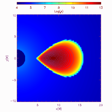
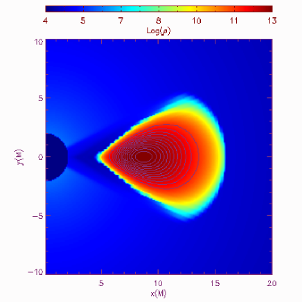
Figure 1: Isocontours of the logarithm of the rest-mass density for the unperturbed model $S2$. The left panel shows the configuration at the initial time and the right panel the corresponding distribution after $100$ orbital timescales. The equilibrium solution is preserved to high accuracy.

Once the specific angular momentum is fixed, the inner edge of the torus $r_{\rm in}$ is determined by the potential gap at such inner edge, $\Delta W_{\rm in}=W_{\rm in}-W_{\rm cusp}$ which, in the case of constant specific angular momentum distributions, is defined as

$$\Delta W_{\rm in}=\ln[(-u_{t})_{\rm in}]-\ln[(-u_{t})_{\rm cusp}],$$ (35)

with $\Delta W_{\rm in}=0$ corresponding to a torus filling its outermost equipotential surface.

All of the models are built with an adiabatic index $\Gamma=4/3$ to mimic a degenerate relativistic electron gas, and the polytropic constant $\kappa$ is fixed such that the torus-to-black hole mass ratio, $M_{\mathrm{t}}/M$, is roughly 0.1. Since the mass of the torus is at most 10$\%$ of that of the black hole, we can neglect the self-gravity of the torus and study the dynamics of such objects in a fixed background spacetime (test-fluid approximation). Moreover, the disc-to-hole mass ratio adopted here is in agreement with the one obtained in simulations of unequal mass binary neutron star mergers performed by Shibata et al. (2003) and Shibata & Sekiguchi (2005).

Overall, we have investigated a number of different models for tori orbiting either nonrotating or rotating black holes. In the case of Schwarzschild black holes, the main difference among the models is the strength of the toroidal magnetic field, which is parametrized by the ratio of the magnetic-to-gas pressure at the centre of the disc, $\beta_{\rm c}\equiv b^{2}/(2p)$. In the case of Kerr black holes, on the other hand, we report results for tori orbiting around black holes with spins $a=0.5,0.7$ and 0.9, while keeping constant the magnetic-to-gas pressure ratio at $\beta_{\rm c}=0.01$. A summary of all the models considered is given in Table 1.

The set of models chosen here will serve a double purpose. Being tori with large average densities, they can provide accurate estimates for the gravitational-wave emission triggered by the oscillations. On the other hand, since the ratio among the eigenfrequencies is the astrophysically most relevant quantity and this does not depend on the density, this set of models is also useful for analysing the oscillation properties of the accretion discs in LMXBs. It is also important to note that for tori with $\beta_{c}>1$ the initial solution degrades over time as a significant mass is accreted in these cases, with an accretion rate that increases with the strength of the magnetic field. The dependence of the stability of thick discs with the strength of the toroidal magnetic field will be the subject of an accompanying paper (Rezzolla et al. (2007)).

The maximum strength of the magnetic field at the centre, determined by the parameter $\beta_{\rm c}$, can be calculated through Eq. (6), which also reflects the dependence of the toroidal magnetic field component on the background metric. The initial models considered are such that $\beta_{\rm c}$ takes values between $0$ and $1$, as shown in Table 1. This also fixes the overall strength of the magnetic field, whose maximum values are reported in the tenth column of the same table. The values of the magnetic field strength at the centre for the case of tori around a Schwarzschild black hole range from the magnetized model $S2$ with $2.50{\times}10^{15}$ Gauss to model $S8$ with $1.85{\times}10^{16}$ Gauss. These values are in good agreement with the typical values expected to be present in the astrophysical scenarios that could form a relativistic thick torus, such as the magnetized core collapse (Cerdá-Durán & Font 2006; Obergaulinger et al. 2006; Shibata et al.2006) and values considered for the collapse of magnetized hypermassive neutron stars by Duez et al. (2006).

In order to trigger the oscillations, we perturb the models reported in Table 1 by adding a small radial velocity (we recall that in equilibrium all velocity components but the azimuthal one are zero). As in our previous work (Zanotti et al. 2003, 2005), this perturbation is parametrized in terms of a dimensionless coefficient $\eta$ of the spherically symmetric accretion flow on to a black hole (Michel 1972), i.e., $v_{r}=\eta(v_{r})_{\rm Michel}$. In all the simulations reported we choose $\eta=0.1$, but the results are not sensitive to this choice as long as the oscillations are in a linear regime (i.e., for $\eta\lesssim 0.2$ Zanotti et al. (2003)).

Finally, it is worth commenting on the choice made for the magnetic field distribution. On the one hand this choice is motivated by the mere convenience of having an analytic equilibrium solution upon which a perturbation can be introduced. On the other hand, there exists an additional motivation which is more astrophysically motivated. As it has been shown in recent simulations of magnetized core collapse (Cerdá-Durán & Font 2006; Obergaulinger et al. 2006; Shibata et al.2006) the magnetic field distribution in the nascent, magnetized, proto-neutron stars has a dominant toroidal component, quite irrespective of the initial configuration. Since gravitational core collapse is one of the processes through which thick accretion discs may form, the toroidal initial configuration of our simulations is well justified. This choice, however, also has an important consequence. Because of the absence of an initial poloidal magnetic field, in fact, the magneto-rotational instability (MRI), which could change even significantly the dynamics of our tori, cannot develop in our simulations. Indeed,  Fragile (2005) has investigated the oscillation of an accretion torus having an initial poloidal magnetic field component. Although preliminary, his results suggest that the development of the MRI and of the Papaloizou-Pringle instability ((Papaloizou & Pringle1984)) may damp significantly the oscillation modes of accretion tori with poloidal magnetic fields. We will address this question in a future work.

6 Results

6.1 Oscillation properties

6.1.1 Dynamics of magnetized tori

Figure 2: Time evolution of the central rest-mass density normalized to its initial value for models $S2$ (left panel) and $S8$ (right panel). Distinctive oscillations are visible during the whole evolution, $t=100\,t_{\mathrm{orb}}$.

We have first investigated equilibrium configurations of magnetized tori by performing numerical evolutions of unperturbed tori ($\eta=0$) and by checking the stationarity of the solution over a timescale which is a couple of orders of magnitude larger that the dynamical one. As representative example, we show in Fig. 1 the isocontours of the logarithm of the rest-mass density of model $S2$ as computed at the initial time $t=0$ (left panel) and at the time when the simulation was stopped (right panel). This corresponds to $t=100\,t_{\mathrm{orb}}$, where $t_{\mathrm{orb}}$ is the Keplerian orbital time for a particle in a circular orbit at the centre of the torus. Aside from the minute accretion of matter from the cusp towards the black hole (see below), the final snapshot of the rest-mass distribution clearly shows the stationarity of the equilibrium initial solution. More precisely, the central rest-mass density, after a short initial transient phase, settles down to a stationary value which differs after 100 orbital timescales only of 2$\%$ from the initial one. This provides a strong evidence of the ability of the code to keep the torus in equilibrium for evolutions much longer than the characteristic dynamical timescales of these objects.

On the left panel of Fig. 2 we show instead the evolution over $100\,t_{\mathrm{orb}}$ of the central rest-mass density of the least magnetized model $S2$, when a perturbation with parameter $\eta=0.1$ is added to the equilibrium model. It is interesting to note that despite the presence of a rather strong toroidal magnetic field, the persistent oscillatory behaviour found in these simulations is very similar to the one found in purely hydrodynamical tori (Zanotti et al. 2003, 2005). Note also that the small secular decrease in the oscillation amplitude is not to be related to numerical or physical dissipation, since the code is essentially inviscid and the EOS used is isoentropic. Rather, we believe it to be the result of the small but nonzero mass spilled through the cusp at each oscillation (see also discussion below). Furthermore, on a smaller timescale than the one shown in Fig. 2, the oscillations show a remarkable harmonic behaviour and this is highlighted in the small insets in Fig. 2. This is in stark contrast with the results of Fragile (2005), which were obtained with comparable numerical resolutions, but with an initial poloidal magnetic field configuration. In that case, in fact, the oscillations were rapidly damped in only a few orbital periods.

Results from a representative model with a higher magnetic field are shown in the right panel of Fig. 2, which again reports the evolution of the normalized central rest-mass density for model $S8$. Note that despite this model has a magnetic-to-gas pressure ratio at the centre $\beta_{c}=1$, and hence a central magnetic field of $\sim 2\times 10^{16}$ G, its overall the dynamics is very similar to that of model $S2$. Also in this case, in fact, the oscillations are persistent during the entire evolution ($100\,t_{\mathrm{orb}}$) and show almost no damping. However, the amplitude does show variations over time and, most importantly, it no longer maintains a symmetric behaviour between maxima and minima, as a result, we believe, of the increased mass accretion through the cusp. We recall, in fact, that all the initial models considered in our sample correspond to marginally stable tori, i.e., tori filling entirely their outermost closed equipotential surface. Any perturbation, however small, will induce some matter to leave the equipotential surface through the cusp, leading to the accretion of mass and angular momentum onto the black hole. Evidence in favour of this is shown in Fig. 3, which reports the accretion mass-flux for model $S2$ (upper panel) and $S8$ (lower panel). While both reflect the oscillations in the dynamics, they also have different mean values, with the one relative to model $S8$ being almost an order of magnitude larger. Note also the correlation between the fluctuations in the mass-accretion rate and the changes in the oscillation amplitudes shown in Fig. 2. In particular, the sudden change in the mass-flux of model $S8$ at $t\sim 35\,t_{\mathrm{orb}}$ and which corresponds to a change in the amplitude modulation in the right panel of Fig. 2.

Although the accretion-rates are well above the Eddington limit (which is $\sim 10^{-16}\ M_{\odot}/{\mathrm{s}}$ for a $2.5\;M_{\odot}$ black hole), the amounts of mass accreted by the black hole at $t=100\,t_{\mathrm{orb}}$ is only 1.3$\%$ and 3.3$\%$ of the initial mass for models $S2$ and $S8$, respectively. Similarly, the total amount of angular momentum accreted at the end of the simulation would introduce a change in the black-hole’s spin of less than $1\%$ for both models $S2$ and $S8$. Overall, therefore, these changes in the mass and spin of the black holes are extremely small and thus justify the use of a fixed background spacetime. Finally, in Fig. 4 we show the evolution of the normalized central rest-mass density for model $K2$, which corresponds to a torus orbiting around a Kerr black hole with spin $a=0.7$. Again, a perturbation with parameter $\eta=0.1$ was added to the equilibrium model so as to investigate the oscillatory behaviour of the torus around its equilibrium position. As in the purely hydrodynamical case, the qualitative behaviour in models around a Kerr black hole is very similar to that found for models around a Schwarzschild black hole, and the dynamics shows, also in this case, a negligible damping of the oscillations after the initial transient.

Figure 3: Time evolution of the mass accretion rate for models $S2$ and $S8$.

6.1.2 Power Spectra

An important feature of axisymmetric $p$-mode oscillations of accretion tori is that the lowest-order eigenfrequencies appear in the harmonic sequence $2:3$. This feature was first discovered in the purely hydrodynamical numerical simulations of Zanotti et al. (2003), subsequently confirmed through a perturbative analysis in a Schwarzschild spacetime by  Rezzolla et al. (2003b), and later extended to a Kerr spacetime and to more general distributions of the specific angular momentum by Zanotti et al. (2005) and Montero et al. (2004). Overall, it was found that the $2:3$ harmonic sequence was present with a variance of $\sim 10\%$ for tori with a constant distribution of specific angular momentum and with a variance of $\sim 20\%$ for tori with a power-law distribution of specific angular momentum. Since the $2:3$ harmonic sequence is the result of global modes of oscillation, it depends on a number of different elements that contribute to small deviations from an exact relation among integers. The latter, in fact, should be expected only for a perfect one-dimensional cavity, trapping the $p$ modes without losses. In practice, however, factors such as the vertical size of the tori, the black hole spin, the distribution of specific angular momentum, the EOS considered, and the presence of a small but nonzero mass-loss, can all influence this departure.

While the understanding of the properties of these modes of oscillation has grown considerably over the last few years (see Montero et al. (2004) for a list of references), and an exhaustive analysis has been made in the case of relativistic slender tori (Blaes et al. (2006)), it was not obvious whether such a harmonic sequence would still be present in the case of magnetized discs with toroidal magnetic fields. To address this question, we have performed a Fourier analysis of the time evolution of some representative variables and obtained quantitative information on the quasi-periodic behavior of the tori. In particular, for all of the models considered, we have Fourier-transformed the evolution of the $\rm{L_{2}}$ norm of the rest-mass density, defined as $||\rho||_{2}\equiv\sum_{i=1}^{N_{r}}\sum_{j=1}^{N_{\theta}}(\rho_{ij})^{2}$ and studied the properties of resulting power spectra. These, we recall, show distinctive peaks at the frequencies that can be identified with the quasi-normal modes of oscillation of the disc. Clearly, the accuracy in calculating these eigenfrequencies depends linearly on the length of the timeseries and is of $0.01\mathrm{\ kHz}$ for the evolutions carried out here and that extend for $100\,t_{\mathrm{orb}}\sim 100\,$ms.

Figure 4: Time evolution of the central rest-mass density normalized to its initial value for the model $K2$

In Fig. 5 we present the power spectra (PSD) obtained from the $\rm{L_{2}}$ norm of the rest-mass density for model $S2$ (left panel) and $S8$ (right panel); in both panels the solid lines refer to the magnetized tori, while the dashed ones to the unmagnetized counterpart $S1$, which is shown for reference. A rapid look at the panels in Fig. 5 reveals that the overall dynamics of magnetized tori shows features which are surprisingly similar to those found by Zanotti et al. (2003, 2005) for unmagnetized accretion tori. Namely, the spectra have a fundamental mode $f$ (which is the magnetic equivalent of the $p$ mode discussed in Zanotti et al. (2003, 2005)) and a series of overtones, for which, in particular, the first overtone $o_{1}$ can usually be identified clearly. Interestingly, also these spectra show the $2:3$ harmonic relation between the frequencies of the fundamental mode and its first overtones. Such a feature remains therefore unmodified and an important signature of the oscillations properties of magnetized tori with a toroidal magnetic field.

Figure 5: Solid lines: Power spectrum of the L-2 norm of the rest-mass density for models $S2$ (left panel) and $S8$ (right panel). The dashed lines show the corresponding PSD for the unmagnetized versions of both models. The units in the vertical axis are arbitrary and the PSDs were obtained using a Hanning filter.

It is also worth noting that in the case of mildly magnetized tori, such as model $S2$, the similarity in the PSD is rather striking and the two spectra differ only in the relative amplitude between the eigenfrequencies $o_{1},o_{2},\ldots$ and the modes which are the result of nonlinear coupling (e.g., $2f-o_{1},2f,\ldots$). On the other hand, in the case of more highly magnetized tori, such as model $S8$, the magnetic field strength is sufficiently large to produce variations in the eigenfrequencies, which are all shifted to higher frequencies, with deviations, however, which become larger for higher overtones. While not totally unexpected [a magnetic field is known to increase the eigenfrequencies of magnetized stars (Nasiri & Sobouti (1989))], these represent the first calculations of the eigenfrequencies of relativistic magnetized discs and, as such, anticipate analogous perturbative studies.

As a way to quantify the differential shift of the eigenfrequencies to larger values, we report in Table 2 the frequencies of the fundamental mode, of the first overtone, and their ratio for all of the models considered. Another analogy worth noticing in the spectra presented in Fig. 5, is the presence of nonlinear couplings among the various oscillation modes. These modes were first pointed out by Zanotti et al. (2005) in the investigation of the dynamics of purely hydrodynamical tori with nonconstant specific angular momentum in Kerr spacetime, and are the consequence of the nonlinear coupling among modes, in particular of the $f$ and $o_{1}$ modes.

Table 2: From left to right, the columns report the name of the model, the frequency of the fundamental mode, the frequency of the first overtone, their ratio, and the magnetic-to-gas pressure ratio at the centre of the torus.

Model	$f$ (Hz)	$o_{1}$ (Hz)	$o_{1}/f$	$\beta_{c}$
$S1$	224	332	1.48	0.00
$S2$	224	332	1.48	0.01
$S3$	228	336	1.47	0.02
$S4$	229	333	1.45	0.04
$S5$	230	330	1.43	0.10
$S6$	230	340	1.48	0.20
$S7$	233	345	1.48	0.50
$S8$	235	341	1.45	1.00
$K1$	275	418	1.52	0.01
$K2$	370	560	1.51	0.01
$K3$	255	404	1.58	0.01

We complete our discussion of the spectral properties of these oscillating discs, by showing in Fig. 6 the PSD for model $K2$, which, we recall, represents a torus orbiting around a Kerr black hole with spin $a=0.7$. As for the previous spectra, the dashed line corresponds to the unmagnetized version of model $K2$ and is included for reference. Overall, the features observed in a Kerr background are very similar to those found for models in the Schwarzschild case. Also in this case, in fact, the fundamental mode, its first overtones and the nonlinear harmonics are clearly identified and no evidence appears of new modes related to the presence of a toroidal magnetic field.

As a final remark we note that the $2:3$ ratio among the different $p$ modes has a relevance also in a wider context. We recall, in fact, that among the several models proposed to explain the QPOs observed in LMXBs containing a black hole candidate, the one suggested by Rezzolla et al. (2003a) is particularly simple and is based on the single assumption that the accretion disc around the black hole terminates with a sub-Keplerian part, i.e a torus of small size. A key point of this model is the evidence that in these objects the frequencies of the fundamental mode and the first overtone are in the $2:3$ harmonic sequence in a very wide space of parameter. The simulations presented here further increase this space, extending it also to the case of magnetized tori and thus promoting the validity of this model for QPOs to a more general and realistic scenario.

6.2 Gravitational-wave emission

As pointed out by Zanotti et al. (2003) the oscillating behavior of perturbed accretion tori is responsible for significant changes of their mass quadrupole moment. As a result, these changes determine the emission of potentially detectable gravitational radiation if the tori are compact and dense enough. This could be the case if the tori are produced via binary neutron star mergers or via gravitational collapse of the central core of massive stars. In this section, we extend the analysis of Zanotti et al. (2003, 2005) for unmagnetized discs and investigate the gravitational-wave emission from constant angular momentum magnetized tori orbiting around black holes.

Although more sophisticated approaches involving perturbative techniques around black holes can be employed to study the gravitational-wave emission from these tori (Nagar et al. (2005); Ferrari et al. (2006); Nagar et al. (2007)), we here resort to the simpler and less expensive use of the Newtonian quadrupole approximation (Zanotti et al. (2003)), which has been suitably modified to account for the presence of a magnetic field, as done by Kotake et al. (2004). In particular, the quadrupole wave amplitude $A_{20}^{\rm E2}$, and which is the second time derivative of the mass quadrupole moment, is computed through the “stress formula” (Obergaulinger et al. (2006))

$$\hskip-14.22636ptA_{20}^{\rm E2}=k\!\int\!\!r^{2}{\rm d}r{\rm d}z\bigg{[}(f_{rr}(3z^{2}\!-\!1)\!+\!f_{\theta\theta}(2\!-\!3z^{2})\!-\!f_{\phi\phi}$$

$$\quad-6zf_{r\theta}\sqrt{1\!-\!z^{2}}\biggl{.}-r\rho\frac{\partial\Phi}{\partial r}(3z^{2}\!-\!1)+3z\rho\frac{\partial\Phi}{\partial\theta}\sqrt{1\!-\!z^{2}}\bigg{]}\;,$$

where $k=16\pi^{3/2}/\sqrt{15}$, $z\equiv\cos\theta$, $f_{ij}\equiv\rho v_{i}v_{j}-b_{i}b_{j}$, and $\Phi$ is the gravitational potential, and is approximated at the second post-Newtonian order from the metric function $g_{rr}=1-2\Phi+2\Phi^{2}$.

Figure 6: As Fig. 5 but for model $K2$.

Figure 7 shows a spectral comparison between the designed strain sensitivity of the gravitational-wave detectors Virgo and LIGO, and the logarithm of the power spectrum $|h(f)|\sqrt{f}$ of the gravitational-wave signals for models $S2$, $S8$, and $K2$ (similar graphs are obtained also for the other models). Note that all of the sensitivity curves displayed in this figure assume an optimally incident wave in position and polarization (as obtained by setting the beam-pattern function of the detector to one), and that the sources are assumed to be located at a distance of 10 kpc.

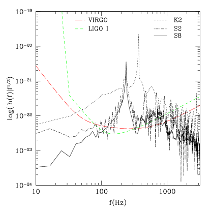
Figure 7: Comparison between the power spectrum $|h(f)|\sqrt{f}$ of the wave signal for models $S2$, $S8$, and $K2$ and the strain sensitivity of LIGO (dashed line), Virgo (long-dashed line).

From Fig. 7 it is clear that all our models lie well above the sensitivity curves of the detectors for galactic sources and also that there are no significant differences in the power spectra as the magnetic field strenght is increased. Interestingly, however, the signal from a torus orbiting around a Kerr black hole is clearly distinguishable from the one around a Schwarzschild black hole. Besides having a fundamental mode at higher frequencies, in fact, also the amplitude is about one order of magnitude larger as a result of it being closer to the horizon and with a comparatively larger central density. As expected from the similarities in the dynamics, the signal-to-noise of these magnetized models is very similar to one of the corresponding unmagnetized tori, and we refer to Zanotti et al. (2005) for a detailed discussion.

7 Conclusions

We have presented and discussed the results of numerical simulations of the dynamics of magnetized relativistic axisymmetric tori orbiting in the background spacetime of either Schwarzschild or Kerr black holes. The tori, which satisfy a polytropic equation of state and have a constant distribution of the specific angular momentum, have been built with a purely toroidal magnetic field component. The self-gravity of the discs has been neglected and, as the models considered are all marginally stable to accretion, the minute accretion of mass and angular momentum through the cusp is not sufficient to affect the background black hole metric.

The use of equilibrium solutions for magnetized tori around black holes has allowed us to study their oscillation properties when these are excited through the introduction of small perturbations. In particular, by considering a representative sample of initial models with magnetic-field strengths that ranged from $2.5\times 10^{15}$ G up to equipartition, and GRMHD evolutions over 100 orbital periods, we have studied the dynamics of these discs and how this is affected by a magnetic field.

Overall, we have found the behaviour of the magnetized tori to be very similar to the one shown by purely hydrodynamical tori (Zanotti et al. (2003, 2005)). As in the hydrodynamical case, in fact, the introduction of perturbations triggers quasi-periodic oscillations lasting tens of orbital periods, with amplitudes that are modified only slightly by the small loss of matter across the cusp. The absence of an inital poloidal magnetic field has prevented the development of the magneto-rotational instability, which could influence the oscillation properties and thus alter our conclusions (Fragile (2005)). Determining whether this is actually the case will be the focus of a future work, where a more generic magnetic field configuration will be considered.

As for unmagnetized tori, the spectral distribution of the eigenfrequencies shows the presence of a fundamental $p$-mode and of a series of overtones in a harmonic ratio $2:3:\dots$. The analogy with purely hydrodynamical simulations extends also to the nonlinear harmonics in the spectra and that are the consequence of the nonlinear coupling among modes, (in particular the $f$ mode and of its first overtone $o_{1}$). Also for them we have found a behaviour which is essentially identical to that found in unmagnetized discs. In summary, no new modes have been revealed by our simulations, and in particular no modes which can be associated uniquely to the presence of a magnetic field. Nevertheless, the influence of the magnetic field is evident when considering the absolute values of the eigenfrequencies, which are shifted differentially to higher frequencies as the strength for the magnetic field is increased, with an overall relative change which is $\sim 5\%$ for a magnetic field near equipartition.

Besides confirming the unmagnetized results, the persistence of the $2:3$ ratio among the different $p$ modes also has an important consequence. It allows, in fact, to extend to a more general and realistic scenario the validity of the QPO model presented by Rezzolla et al. (2003a) and Schnittman & Rezzolla (2006), and which explains the QPOs observed in the x-ray luminosity of LMXBs containing a black hole candidate with the quasi-periodic oscillations of small tori near the black hole. The evidence that this harmonic ratio is preserved even in the presence of toroidal magnetic fields, provides the model with additional robustness.

When sufficiently massive and compact, the oscillations of these tori are responsible for an intense emission of gravitational waves and using the Newtonian quadrupole formula, conveniently modified to account for the magnetic terms in the stress-energy tensor, we have computed the gravitational radiation associated with the oscillatory behaviour. Overall, we have found that for Galactic sources these systems could be detected as they lie well within the sensitivity curves of ground-based gravitational-wave interferometers.

As a concluding remark we note that our discussion here has been limited to tori with magnetic fields whose pressure is at most comparable with the gas pressure, i.e., $\beta_{c}\leq 1$. The reason behind this choice is that while in equilibrium, the magnetized tori with a purely toroidal magnetic field are not necessarily stable. Rather, indications coming both perturbative calculations and from nonlinear simulations, suggest that these tori could be dynamically unstable for sufficiently strong magnetic fields. The results of these investigations will be presented in a forthcoming paper (Rezzolla et al. (2007)).

References

- (1) Abramowicz M. A. Jaroszyński M. & Sikora M., 1978, A&A, 63, 221.
- Anninos et al. (2005) Anninos P., Fragile P. C., Salmonson J. D., 2005, ApJ, 635, 723
- (3) Antón L., Zanotti O., Miralles J. A., Martí J. M., Ibáñez J. M., Font J. A., Pons J. A., 2006, ApJ, 637, 296
- (4) Evans C., Hawley J. F., 1988, ApJ, 207, 962
- Balbus (2003) Balbus S. A., Ann. Rev. Astron. Astrophy., 41, 555-597
- Blaes et al. (2006) Blaes O. M., Arras P., Fragile 2006, MNRAS, 369 1235
- Cerdá-Durán & Font (2006) Cerdá-Durán P., Font J.A., 2007, submitted to the CQG special issue based on New Frontiers in Numerical Relativity conference
- De Villiers et al. (2003) De Velliers J. P., Hawley J. F., Krolik J. H., 2003, ApJ, 599, 1238
- De Villiers & Hawley (2003) De Villiers J., Hawley J. F., 2003, ApJ, 589, 458
- Duez et al. (2005) Duez M. D., Liu Y. T., Shapiro S. L., Stephens B. C., 2005, Phys. Rev. D, 72, 024028
- Duez et al. (2006) Duez M. D., Liu Y. T., Shapiro S. L.,Shibata M., Stephens B. C., 2006, Phys. Rev. Lett., 96, 031101
- Ferrari et al. (2006) Ferrari V., Gualtieri L., Rezzolla L., Phys. Rev. D 73 124028 (2006)
- Font & Daigne (2002) Font J. A., Daigne F., 2002a, MNRAS, 334, 383
- Fragile (2005) Fragile P. C., 2005, astro-ph/0503305
- Gammie, McKinney & Tóth (2003) Gammie, C. F., McKinney, J. C., Tóth, G., 2003, ApJ,589, 444
- (16) Giacomazzo, B., Rezzolla, L., 2007, Class. Quantum Grav. submitted, gr-qc/0701109
- Kozlowski et al. (1978) Kozlowski M., Jaroszynski M., Abramowicz M. A., 1978, A&A, 63, 209
- Komissarov (2005) Komissarov S. S., 2005, MNRAS, 359, 801
- Komissarov (2006) Komissarov S. S., 2006, MNRAS, 368, 993
- Kotake et al. (2004) Kotake K., Sawai H., Yamada S., Sato K., 2004, ApJ, 608, 391
- Landau & Lifschitz (1976) Landau L. D., & Lifshitz E. M., Mechanics, 1976, Oxford, Pergamon Press
- McKinney (2006) McKinney J. C., 2006, MNRAS, 368, 1561
- Michel (1972) Michel F., 1972, Astrophys. Spa. Sci., 15, 153
- Mizuno et al. (2006) Mizuno Y., Nishikawa K.-I., Koide S., Hardee P., Fishman, G. J., 2006, astro-ph/0609004
- Mönchmeyer et al. (1991) Mönchmeyer R., Schäfer G., Müller E., Kates R. E., 1991, A&A, 246, 417
- Montero et al. (2004) Montero P.J., Rezzolla L., Yoshida S’i., 2004, MNRAS, 354, 1040
- Nagar et al. (2005) Nagar A., Font J. A., Zanotti O. & De Pietri R., Phys. Rev. D 72, 024007 (2005)
- Nagar et al. (2007) Nagar A., Zanotti O., Font J .A., & Rezzolla L., Phys. Rev. D (2007) 75, 044016
- Nasiri & Sobouti (1989) Nasiri S., Sobouti Y., 1989, A&A, 217, 127
- Obergaulinger et al. (2006) Obergaulinger M., Aloy M. A., Müller E., 2006, A&A, 450, 1107
- Okada et al. (1989) Okada R.,Fukue J., Matsumoto R., 1989 PASJ, 41, 133-140
- (32) Papaloizou J. C. E.,Pringle J. E., 1984 MNRAS, 208,721
- Rezzolla et al. (2003a) Rezzolla L., Yoshida S’i., Maccarone T. J., Zanotti O., 2003a MNRAS, 344, L37
- Rezzolla et al. (2003b) Rezzolla L., Yoshida S’i., Zanotti O., 2003b, MNRAS, 344, 978
- Rezzolla et al. (2007) Rezzolla L., Yoshida S’i., Zanotti O., Montero P., & Font J. A., 2007 in preparation
- (36) Ryu, D., Miniati, F., Jones, T. W., & Frank, A. 1998, ApJ, 509, 244
- Schnittman & Rezzolla (2006) Schnittman, J. .D, Rezzolla L., 2006 ApJ, 637, L113
- Shakura & Sunyaev (1973) Shakura N. I., Sunyaev R. A., 1973, A&A, 24, 337
- Shibata et al. (2003) Shibata M., Taniguchi K., Uryū K., 2003, Phys. Rev. D, 68, 084020
- Shibata & Sekiguchi (2005) Shibata M., Sekiguchi Y.-I., 2005, Phys. Rev. D, 72, 044014
- (41) Shibata M., Liu Y. T., ,Shapiro S. L. & Branson C. S.,2006, Phys. Rev. D, 74 104026
- Zanotti et al. (2003) Zanotti O., Rezzolla L., Font J .A., 2003, MNRAS, 341, 832
- Zanotti et al. (2005) Zanotti O., Font J .A., Rezzolla L., Montero P. J., 2005, MNRAS, 356, 1372