Application of the Probability Event Horizon filter to constrain the local rate density of binary black hole inspirals with Advanced LIGO

Abstract

The temporal evolution of the gravitational wave background signal resulting from stellar-mass binary black hole (BBH) inspirals has a unique statistical signature. We describe the application of a new filter, based on the ‘probability event horizon’ (PEH) concept, that utilizes both the temporal and spatial source distribution to constrain the local rate density, $r_{0}$, of BBH inspiral events in the nearby Universe. Assuming Advanced LIGO sensitivities and an upper rate of Galactic BBH inspirals of $30\hskip 2.84526pt\mathrm{Myr}^{-1}$, we simulate GW data and apply a fitting procedure to the PEH filtered data. To determine the accuracy of the PEH filter in constraining $r_{0}$, a comparison is made with a fit to the brightness distribution of events. We apply both methods to a data stream containing a background of Gaussian distributed false alarms. We find that the brightness distribution yields lower standard errors, but is biased by the false alarms. In comparison the PEH method is less prone to errors resulting from false alarms but has a lower resolution as fewer events contribute to the data. Used in combination, the PEH and brightness distribution methods provide an improved estimate of the rate density.

1 Introduction

The LIGO gravitational wave (GW) detectors are currently taking data at design sensitivity, and embarking on long science runs. Promising GW sources potentially detectable by LIGO are coalescing binary systems containing neutron stars (NSs) and/or black holes (BHs)– see Flanagan & Hughes (1998), Miller et al. (2004), Thorne (1995). Because of the enormous GW luminosity $\sim 10^{-3}c^{5}/G\sim 10^{23}L_{\odot}$, binary black hole (BBH) inspirals are among the most promising candidates for a first detection of GWs (Baker et al., 2002; Flanagan & Hughes, 1998; Sathyaprakash, 2004; Burger et al., 2005).

For LIGO-type detectors, even highly energetic BBH inspirals are predicted to be detected at a rate of only $(10^{-3}-0.6)\hskip 1.42262pt\mathrm{yr}^{-1}$ (Cutler and Thorne, 2002). However, the next generation of interferometric detectors, planned to go online in the next decade, should be sensitive to an abundance of sources, with event rates 1000 times greater than current detectors. These ‘Advanced’ interferometers will provide a new window to the cosmos not accessible by conventional astronomy.
The introduction of advanced detectors will allow us to detect BBH inspiral events out to a distance of $z\approx 0.4$. Events within this volume will contribute to the low probability ‘popcorn’ component of the astrophysical GW background for BBHs. It has been shown that the temporal and spatial distribution of transient sources which form this part of the GW background can be described by the Probability Event Horizon (PEH) concept of Coward & Burman (2005).
The PEH describes the temporal evolution of the brightness of a class of transient events. The probability of a nearby event accumulates with observation time, so that the peak event amplitude has a statistical distribution dictated by the rate density and spacetime geometry. This feature provides a tool to model the detectability of a distribution of transient GW sources. Coward et al. (2005) used the PEH to model the detectability of NS inspirals as a function of observation time assuming LIGO and Advanced LIGO sensitivities and reasonable estimates of the local rate density of events in the nearby Universe, $r_{0}$.
In this study we consider the use of the PEH method to determine the local rate density of BBH coalescence events. We use a cosmological model to create synthetic data corresponding to four months data at advanced LIGO sensitivity. We then attempt to recover the assumed rate density.
First we use the conventional approach of studying the brightness distribution of all events. This method does not make use of the time evolution. It simply utilizes the number-amplitude distribution and fits the observations to the rate density. We compare this with the PEH method, which utilizes the temporal distribution of events. For simplicity, we use a standard candle approximation to model our source population. We note that a network of detectors would allow us to exploit a special property of compact binary inspiral events, for which the chirp signal provides a measure of the luminosity distance to the source, enabling such sources to be treated as standard candles (Schutz, 1986; Sathyaprakash, 2004; Chernoff & Finn, 2003; Finn, 1993).

To test both methods, we simulate a candidate population of BBH inspiral events by approximating the output data stream resulting from matched filtering. A simplified detection model (described in Section 5.1) is used which assumes Gaussian detector noise. We use the candidate population to show that the temporal evolution of events has a unique statistical signature and exploit this signature to constrain $r_{0}$. To determine the effect of detector efficiency we apply both methods to data corresponding to high and low false alarm rates. We also consider the effect of different star formation rate (SFR) models and determine bias introduced by different SFR evolution functions.
The paper is organized as follows: In Section 2 we review event rate predictions and then discuss the evolution of the event rate of BBH inspirals in Section 3. In Section 4, we explain the PEH concept and show how it can be used to probe the source rate density and to differentiate between different astrophysical populations of sources. We describe the simulation of candidate events in Section 5 and use these data in Section 6 to determine an estimate of $r_{0}$ using the brightness distribution of sources. In Section 7 we present a method for extracting PEH data and use least-squares fitting to constrain $r_{0}$. We present our results in Section 8 and in Section 9 summarize the key findings and discuss how this work can be extended.

2 EVENT RATE ESTIMATIONS

The local rate density of a particular astrophysical GW source is fundamental to estimating the number of potentially observable events. Usually defined within a volume spanning the Virgo cluster of galaxies, the local rate density, $r_{0}$, is determined using estimated source rates within a larger fixed volume of space.

In the case of NS-NS inspirals, current rate estimates rely on a small sample of sources. The discovery of the double pulsar PSR J0737 – 3039, with estimated coalescence time $\sim 87$ Myr, increased the estimated inspiral rate for double NSs in our Galaxy by about an order-of-magnitude to $20-300\hskip 2.84526pt\mathrm{Myr}^{-1}$ (Burgay et al., 2003; Kalogera et al., 2004) with respect to earlier estimates (Kalogera et al., 2001; Phinney, 1991).

The rates of BBH systems are even more uncertain. Because these systems have not been observed directly, their evolutionary parameters can be obtained only though population synthesis, which predicts Galactic event rates $\leq 10^{-1}-80\hskip 1.42262pt\mathrm{Myr}^{-1}$. However, GW emissions from BBH will be detectable out to much greater distances than other systems of coalescing compact objects (Sathyaprakash, 2004). The rates of BH-NS inspirals are of a similar range to those of BH - BH systems, but have lower expected detection rates as a result of their less energetic emissions.

In this study, we use the Galactic BBH coalescence rate ${\cal R}_{\rm gal}^{BBH}\sim 30\hskip 2.84526pt\mathrm{Myr}^{-1}$, obtained from the standard model in the population synthesis calculations of Belczynski et al. (2002). We note that this rate is an upper limit. We convert this to a rate per unit volume, $r_{0}$, using the conversion factor $10^{-2}$ from Ando (1999) for the number density of galaxies in units of $\mathrm{Mpc}^{-3}$, yielding the reference value of the local rate density, $\tilde{r}_{0}=0.3\hskip 2.84526pt\mathrm{Myr}^{-1}\hskip 1.42262pt\mathrm{Mpc}^{-3}$, which we will employ in this study.

Rate estimates will benefit greatly from the introduction of advanced GW detectors, which will allow unobscured source counts to be conducted to almost cosmological volumes. A network of detectors will improve the sky coverage and source localization. A network may employ coherent analysis, in which synchronized detector outputs are merged (Finn, 2001) before a search for a common pattern, or alternatively, a coincidence analysis, in which individual events from different detectors are correlated in time (Arnaud et al., 2002). However, as a result of the non-uniform antenna patterns, even a network of three detectors of similar sensitivity will have difficulty obtaining maximum efficiency (Arnaud et al., 2003a). In addition, the efficiency of a detector network for a particular source type will depend on the false alarm rate and the signal-to-noise threshold for detection – therefore high number counts may be balanced by an increased rate of false alarms. We will investigate this in Section 6.

3 THE BBH COALESCENCE RATE EVOLUTION

3.1 The event rate equation

For standard Friedman cosmology a differential event rate in the redshift shell $z$ to $z+{\mathrm{d}}z$ is given by:

$$\mathrm{d}R=\frac{\mathrm{d}V}{\mathrm{d}z}\frac{r_{0}e(z)}{1+z}\mathrm{d}z\,,$$ (1)

where $\mathrm{d}V$ is the cosmology-dependent co-moving volume element and $R(z)$ is the all-sky ($4\pi$ solid angle) event rate, as observed in our local frame, for sources out to redshift $z$. Source rate density evolution is accounted for by the dimensionless evolution factor $e(z)$, normalized to unity in our local intergalactic neighbourhood, and $r_{0}$ is the $z=0$ source rate density. The $(1+z)$ factor accounts for the time dilation of the observed rate by cosmic expansion, converting a source-count equation to an event rate equation.

The cosmological volume element is obtained by calculating the luminosity distance from (cf. Peebles (1993), p. 332)

$$d_{\mathrm{L}}(z)=(1+z)\frac{c}{H_{0}}\int_{0}^{z}\frac{\mathrm{d}z\hskip 1.42262pt^{\prime}}{h(z\hskip 1.42262pt^{\prime})}\,,$$ (2)

and using (Porciani and Madau 2001, eq. 3)

$$\frac{\mathrm{d}V}{\mathrm{d}z}=\frac{4\pi c}{H_{0}}\frac{d_{\mathrm{\hskip 0.7113ptL}}^{\hskip 4.2679pt2}(z)}{(1+z)^{\hskip 0.7113pt2}\hskip 1.42262pth(z)}\hskip 5.69054pt.$$ (3)

The normalized Hubble parameter, $h(z)$, is given by

$$h(z)\equiv H(z)/H_{0}=\big{[}\Omega_{\mathrm{m}}(1+z)^{3}+\Omega_{\mathrm{\Lambda}}\big{]}^{1/2}\,$$ (4)

for a ‘flat-$\Lambda$’ cosmology $(\Omega_{\mathrm{m}}+\Omega_{\mathrm{\Lambda}}=1$). We use $\Omega_{\mathrm{m}}=0.3$ and $\Omega_{\mathrm{\Lambda}}=0.7$ for the $z=0$ density parameters, and take $H_{0}=70$ km s^-1 Mpc^-1 for the Hubble parameter at the present epoch.

3.2 The source rate evolution of BBH

For the source rate evolution factor, $e\hskip 0.85358pt(z)$, we employ three star formation rate (SFR) models and a non-evolving SFR density for comparison. To simulate a candidate population of BBH inspiral events we employ the observation-based SFR model SF2 of Porciani & Madau (2001). Based on observed rest-frame ultraviolet and H$\alpha$ luminosity densities, this model includes an allowance for uncertainties in the amount of dust extinction at high $z$. In order to constrain $r_{0}$ by least-squares fitting to the simulated data, we will use three additional models: a non-evolving SFR density model obtained by setting $e(z)=1$, the model SF1 of Porciani & Madau (2001) and the model SH, based on an analytical fit to hydrodynamic simulations conducted by Springel and Hernquist (2003) in a flat-$\Lambda$ cold dark matter cosmology; SF1 includes an upward correction for dust extinction at high $z$. We re-scale SF1 and SF2, originally modelled in an Einstein-de-Sitter cosmology, to a flat-$\Lambda$ cosmology using the procedure outlined in the appendix of Porciani & Madau.

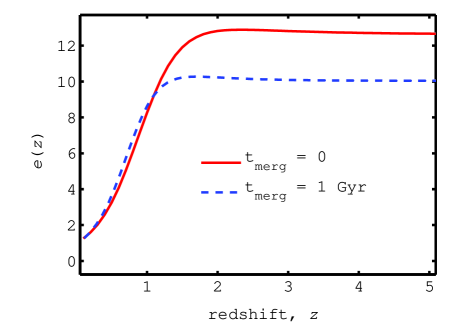
Figure 1: The solid line shows the dimensionless SFR density evolution factor $e(z)$ for the SFR model SF2 of Porciani & Madau (2001) in the flat-$\Lambda$ (0.3, 0.7) cosmology. To allow for the average coalescence time of BBH systems, the dashed line shows the effect of a time delay of 1 Gyr on $e(z)$.

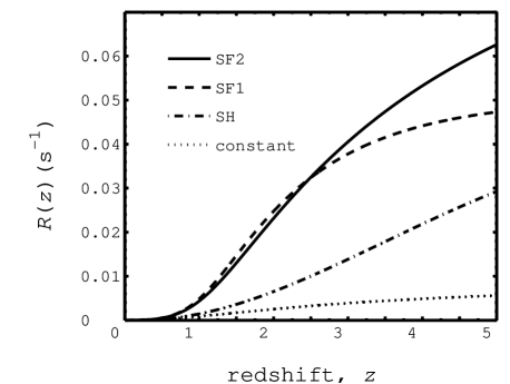
Figure 2: The all-sky BBH coalescence rate as a function of $z$ using a Galactic rate ${\cal{R}}_{\mathrm{Gal}}^{BBH}\sim 30\hskip 2.84526pt\mathrm{Myr}^{-1}$ and merger time of 1 Gyr (Belczynski et al. 2002). We employ the observation-based star formation rate models SF1 and SF2 of Porciani & Madau (2001), a constant (non-evolving) model and a simulation-based model, SH, of Springel and Hernquist (2003).

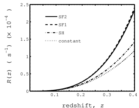
Figure 3: The all-sky rate of BBH coalescence as a function of $z$ as previously shown in Figure 2, but within a distance of $z=0.4$, corresponding to the Advanced LIGO detectability horizon for these sources.

Coward et al. (2005) assumed that the formation of double NS systems closely tracks the evolving star formation rate. They based their assumptions on short merger times and showed that a time delay of up to 5 Gyr had minimal effect on the differential rate of events at low redshift. However, in comparison with NS-NS systems, for which the distribution of merger times has a large range, peaking at around 0.3 Myr (Belczynski et al., 2002), the merger time distributions of BBH systems are predominantly skewed towards longer merger times – from about 100 Myr to the Hubble time (Bulik et al., 2004b).

Belczynski et al. used population synthesis methods to calculate the properties and coalescence rates of compact binaries. They used a range of different scenarios defined by the initial physical parameters of the binary system such as component masses, orbital separations and eccentricities. They also included properties which affect the evolutionary channels of the system, such as mass transfer, mass losses due to stellar winds and kick velocities. Their calculations implied that, compared to NS-NS systems, the wider orbits and stronger dependence of merger time on initial separation for BH-NS and BH-BH systems resulted in longer merger times, mostly in the range 0.1 to several Gyr (Belczynski et al. section 3.4.5).

A standard model was defined by Belczynski et al. (2002) using a range of assumptions, including: a non-conservative mass transfer with half the mass lost by the donor lost by the system; a kick velocity distribution that accounts for the fact that many pulsars have velocities above 500 km $\mathrm{s}^{-1}$; constant Galactic star formation for the last 10 Gyr. For this model they found a distribution in BBH merger times that peaked at  1 Gyr. We therefore take this value as an average merger time and shift $e\hskip 0.85358pt(z)$ to reflect this delay time. Using the method described in section 2 of Coward et al. (2005), we can convert $e(z)$ to a function of cosmic time, $t_{\mathrm{cos}}$, using the relation

$$t_{\mathrm{cos}}(z)=\int_{0}^{z}[\hskip 1.42262pt(1+z\hskip 1.42262pt^{\prime})h(z\hskip 1.42262pt^{\prime})\hskip 1.42262pt]^{-1}\hskip 1.42262ptdz\hskip 1.42262pt^{\prime}\hskip 1.42262pt.$$ (5)

We apply a 1 Gyr time shift and then convert back to a function of $z$. Figure 1 shows the factor $e(z)$ for SF2 with and without the time delay. The result shows that within the range of advanced LIGO, $z\sim 0.4$, $e(z)$ is not significantly altered. Therefore, although we include this time delay in our calculations, within the ranges of advanced LIGO detectors it will not have a significant influence on the results.

Figure 2 shows the all-sky BBH coalescence rate, $R\hskip 1.42262pt(z)$, calculated by integrating the differential rate from the present epoch to redshift $z$. Using SF2, the rate continues increasing to distances well beyond the cosmological volume elements considered in this study. We therefore assume a universal rate of events, $R^{\mathrm{U}}$ (usually defined as the asymptotic value of the all-sky rate as $z$ increases) of $\sim 0.06\hskip 2.84544pt\mathrm{s}^{-1}$ and a corresponding mean temporal interval $\tau=1/R^{\mathrm{U}}=17$ s.

Figure 3 shows the all-sky BBH coalescence rate for sources within Advanced LIGO sensitivities. The potential detection horizon extends to $z=0.4$ and the corresponding mean rate of events is $\sim 2.5\times 10^{-4}\hskip 2.84526pt\mathrm{s}^{-1}$ using SF2. If we assume all sources are composed of two $10M_{\odot}$ black holes, this rate corresponds to around 874 events $\mathrm{yr}^{-1}$ with SNR $\geq 8$.

4 THE PROBABILITY EVENT HORIZON FOR BBH COALESCENCE EVENTS

4.1 The Probability Event Horizon

The rate, as observed in our frame, of transient astrophysical events occurring throughout the Universe, is determined by their spatial distribution and evolutionary history. The distribution of event observation times follows a Poisson distribution and the temporal separation between events follows an exponential distribution defined by the mean event rate. For cosmological events, the rate depends on the cosmology dependent volume and radial distance through redshift, $z$. We assume that an observer measures both a temporal location and a ‘brightness’ for each event, where the brightness is determined by the luminosity distance to the event.

It follows from these assumptions that the probability for at least one event to occur in the volume bounded by $z$, during observation time $T$ at a mean rate $R(z)$ at constant probability $\epsilon$ is given by the exponential distribution:

$$p(n\geq 1;R(z),T)=1-e^{-R(z)T}=\epsilon\,,$$ (6)

$1-e^{-RT}$ being the probability of at least one event occurring (see Coward & Burman 2005).

For equation (6) to remain satisfied as observation time increases, the mean number of events in the sphere bounded by $z$, $N_{\epsilon}=R(z)T=|\mathrm{ln}(1-\epsilon)|$, must remain constant. The PEH is defined by the redshift bound, $z_{\epsilon}^{\mathrm{PEH}}(T)$, required to satisfy this condition.

We note that the for events occurring within a volume bounded by about a few Gpc, the PEH is well approximated using Euclidean geometry and takes on a simple analytical form with $z$ now replaced by the radial distance in flat space:

$$r_{\epsilon}^{\mathrm{PEH}}(T)=(3N_{\epsilon}/4\pi r_{0})^{1/3}T^{-1/3}\;,$$ (7)

where $r_{0}$ is a rate per unit volume. By setting $\epsilon=0.95$, one can generate a threshold corresponding to a 95% probability of observing at least one event within $z_{\epsilon}^{\mathrm{PEH}}(T)$, or alternatively, $r_{\epsilon}^{\mathrm{PEH}}(T)$ for a Euclidean PEH model. We define a ‘null PEH’, representing the 95% probability that no events will be observed within this threshold, by setting $\epsilon=0.05$. When combined, we refer to these two PEHs as the 90% PEH band – that is 90% of events are expected to occur in the region enclosed by the two PEHs. By scaling some fiducial GW amplitude by $d_{\mathrm{L}}(z)$, we express the 90% PEH band as 90% confidence bounds of peak GW amplitude against observation time.

Figure 4 shows the Euclidean 95% PEH curves for BBH, using three different values of $r_{0}$, differing by an order of magnitude. We note that for a particular transient GW source population, the PEH is intrinsically dependent on $r_{0}$. The plot shows that for a particular source type, the PEH model can be used to estimate the value of $r_{0}$.

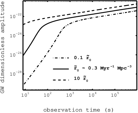
Figure 4: The GW amplitude 95% PEH curves for BBH using three values for the local rate density, $r_{0}$. The PEH curve corresponding to the reference value of the local rate density, $\tilde{r}_{0}$, used in this study is shown by the solid line. An increase in $r_{0}$ by an order of magnitude shifts the PEH curve towards earlier observation times (dashed line). This implies an increased probability for detecting a local high-amplitude event. The dot-dashed line shows that a decrease in $r_{0}$ of the same magnitude has the reverse effect.

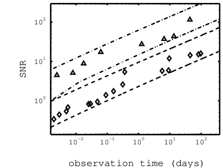
Figure 5: To illustrate that our simulated data is consistent with the PEH model, we show the 90% PEH thresholds (see Section 4.1) and simulated PEH data for two different GW binary inspiral source types with varying event rates recorded within a redshift $z$. The PEH thresholds show the optimal SNR for an Advanced LIGO detector as a function of observation time. We assume a standard-candle approximation based on the fiducial distances for an optimal SNR of 8 for each source. The fiducial distances and universal event rates for the GW populations are: NS-NS inspirals at 200 Mpc and $R^{U}\sim 0.2\hskip 2.84526pt\mathrm{s}^{-1}$(represented by diamonds) and BBH at 2 Gpc and $R^{U}\sim 0.05\hskip 2.84526pt\mathrm{s}^{-1}$(indicated by triangles).

4.2 The PEH filter applied to astrophysical populations

Coward et al. (2005) outlined the PEH filter – a procedure used to extract a cosmological signature from a distribution of events in redshift and time. The concept is very simple: the longer one observes the greater the probability of a nearby event – the PEH filter quantifies this dependence as a means of probing the cosmological rate density. The PEH filter searches for the time dependence of event amplitudes which is imposed by their cosmological distribution. It is a non-linear filter applied to a body of data by recording successively closer events. We will apply the technique to a distribution of amplitudes, $A$, as a function of observation time, $t$, recording the successive $(t_{i},A_{i})$ that satisfy the condition $A_{i+1}>A_{i}$. The resulting events will be referred to as the ‘PEH population’.

By fitting to PEH data we can probe the local rate density of an astrophysical population. We note that just as brightness distributions can be used to separate and identify different source populations, so also can different source populations be identified in PEH plots.

Figure 5 demonstrates this property by comparing synthetic PEH populations of BBH and NS-NS inspirals. For the two source types we use a standard candle approximation based on an optimal SNR of 8 assuming an Advanced LIGO detector with a fiducial distance of 200 Mpc for NS-NS inspirals and 2 Gpc for BBH inspirals.

We show the 90% PEH bands for the two populations as a SNR. It is evident that if the PEH signature of an astrophysical GW background could be extracted from detector noise, the presence of different astrophysical backgrounds could be identified. Clearly this method will only work if the luminosities of the populations differ widely. In reality, different luminosities will also be associated with different waveforms, and there are likely to be more evident differences than the simple luminosity effects.

5 SIMULATING A CANDIDATE POPULATION OF BBH INSPIRALS

5.1 The GW source model

We will consider only the well understood inspiral stage of a BBH coalescence to provide quantitive data for our source model. To model the GW background from BBH inspirals it is sufficient to assume that the raw interferometer data is preprocessed by passing it through an optimal filter. This transforms events into approximate short duration Gaussian pulse signals (Abbott et al., 2004; Shawhan & Ochsner, 2004) embedded in Gaussian detector noise. By injecting a population of simulated events into GW detector noise of Advanced LIGO sensitivity, we approximate the processed output data stream of a GW detector and then apply sub-optimal burst filtering to extract candidate events or ‘triggers’. A more realistic detection pipeline will employ a range of templates representing different BBH mass configurations. To simplify our detection model, we assume a single BBH mass configuration for our sources, representing the output of a fixed template.

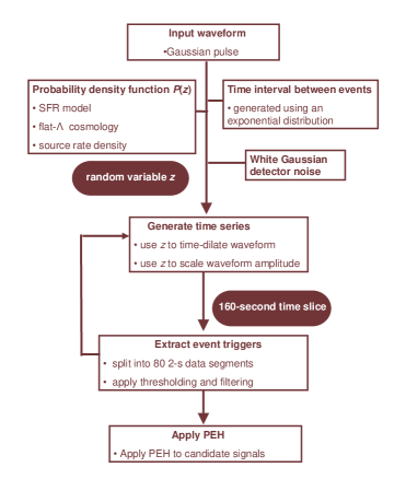
Figure 6: Flow chart outlining the simulation pipeline to generate a candidate population of BBH inspiral events in interferometer detector noise. Individual inspiral events are scaled in amplitude and time-dilated according to the random variable $z$, obtained from the probability distribution shown in Figure 7. The events are injected into simulated detector noise, with the temporal separations between successive events following an exponential distribution. Candidate signals are extracted using amplitude thresholding and robust sub-optimal filtering.

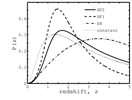
Figure 7: The probability distribution function for BBH inspirals throughout the Universe modelled using the same parameters as for the cumulative rate (see Fig. 2). For SF1, SF2 and the constant (non-evolving) model, the most probable events occur in $z\approx 1-2$. For SH, the most probable events occur significantly earlier, in $z\approx 3-4$, but with a flatter distribution.

To represent the response to BBH events by optimal matched filtering, we adopt as a model waveform the simplified but robust form used by Arnaud et al. (2003b) and Abbott et al. (2005) to model GW burst sources. This is a linearly polarized 5 -ms duration Gaussian pulse, which approximates to the form of the event triggers in processed data from the LIGO S1 search for inspirals (Abbott et al., 2004; Shawhan & Ochsner, 2004). We note that we have chosen to ignore any additional secondary peaks which occur at high SNRs.

The two polarizations of this signal will be given by:

$$h_{+}(t)=A\hskip 1.42262pt\mathrm{exp}\left[{-\frac{\left(\textstyle{t}-\textstyle{t}_{0}\right)^{2}}{\textstyle{2}\textstyle{\Delta}^{2}}}\right],\hskip 5.69054pth_{\times}(t)=0\hskip 1.42262pt\hskip 7.11317pt$$ (8)

with amplitude $A$ and half-width $\Delta$; the time value of the signal maximum, $t_{0}$, is set to 10 ms. The output response, $h(t)$, will be a linear combination of the two polarizations

$$h(t)=F_{+}h_{+}+F_{\times}h_{\times}\hskip 1.42262pt,$$ (9)

where $F_{+}$ and $F_{\times}$ are the antenna pattern functions, which are functions of sky direction, represented by the spherical polar angles $\theta$ and $\phi$, and polarization angle, $\psi$, of the GW signals relative to the detector (Jaranowski et al., 1998).

The filter response amplitude, $A$, will be dependent on the masses of the BBH system. For simplicity, rather than using a distribution of BBH masses, we use a standard source model. Using the BENCH code to model the detector noise spectrum, we approximate the GW amplitude for an optimum SNR of 80 at 200 Mpc.

By assuming a standard BBH system we ignore the amplitude distribution from the BH mass spectrum. However, this assumption is not a limitation to the PEH method because the signature of an inspiralling binary system contains a measure of its luminosity distance (Schutz, 1986; Sathyaprakash, 2004; Finn, 1993; Chernoff & Finn, 2003). Therefore, for a network of GW detectors, the analysis described in this paper could be repeated using luminosity distances rather than amplitudes.

5.2 Simulation of GW interferometer data

The simulation pipeline used to generate a cosmological GW population of BBH inspiral triggers in GW detector noise is shown in Figure 6. We use the BENCH code to calculate the noise sensitivity curve corresponding to our source model.

Following Arnaud et al. (2003b), we define the standard deviation of the detector noise as:

$$\sigma=h_{\mathrm{rms}}\sqrt{f_{\mathrm{o}}/2f_{\mathrm{c}}}\hskip 1.42262pt,$$ (10)

with $h_{\mathrm{rms}}$ the root-mean-square value of the advanced LIGO noise curve at rest frame frequency $f_{\mathrm{c}}$, and $f_{\mathrm{o}}$ the sampling frequency. We assume the noise is white Gaussian with zero mean.

The amplitude and duration of each potential BBH inspiral event is defined by the random variable $z$, generated from a probability density function $P(z)$ for these events. We obtain $P(z)$ by normalizing the differential event rate, $\mathrm{d}R/\mathrm{d}z$, by $R^{U}$, the Universal rate of BBH inspiral events, integrated throughout the cosmos, as seen in our frame (cf. Coward & Burman 2005, section 3):

$$P\hskip 1.42262pt(z)\hskip 1.42262pt{\mathrm{d}}z={\mathrm{d}}R/R^{\mathrm{U}}\;.$$ (11)

Equation 11 defines $P(z)\hskip 1.42262pt\mathrm{d}z$ as the probability that an observed event occurred in the redshift shell $z$ to $z+\mathrm{d}z$. In Figure 7 we present curves for the several star formation rate models. We see that the most probable events will occur at $z\approx 1-2$ for SF1 and SF2. The corresponding cumulative distribution function $C(z)$, giving the probability of an event occurring in the redshift range $0$ to $z$, is the normalized cumulative rate :

$$C(z)=R(z)/R^{\mathrm{U}}\;.$$ (12)

We use $C(z)$ to simulate events and their associated redshifts and hence the GW amplitude of each injected candidate event, $h(t)$, is computed from equation (9). Random values of the antenna response variables, $\theta$, $\phi$ and $\psi$, are simulated and $h(t)$ is scaled inversely by the luminosity distance $d_{\mathrm{L}}(z)$. The signal duration is time-dilated by the factor $(1+z)$.

The temporal distribution of events in our frame is stochastic and the separation of events is described by Poisson statistics. The time interval between successive events, $\tau$, will therefore follow an exponential distribution. Successive waveforms, with amplitude and distance defined by the random variable $z$ are generated and injected into a data pipeline at time intervals $\tau$.

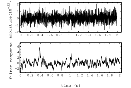
Figure 8: The top panel shows an optimally orientated burst signal (a 5- ms Gaussian pulse) at $t\approx 0.4$ s with an optimal SNR of 8 when embedded in Gaussian noise corresponding to 200 Hz of the Advanced LIGO noise spectrum. The bottom panel shows the response of the mean filter in terms of a SNR. The mean filter response to this signal is about 70% of that of an optimal filter.

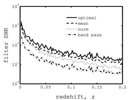
Figure 9: The effective SNR performance of three GW burst filters, as functions of $z$, in identifying the optimally orientated Gaussian pulse signal shown in Fig. 8. Compared with the performance of an optimal filter in Gaussian detector noise with Advanced LIGO sensitivity, the mean and norm filters provide useful performance. Noise samples are generated for each $z$ – SNR fluctuations are the result of RMS variations between noise samples.

5.3 Candidate signal extraction

We restrict ourselves to the well understood coalescence phase of BBH sources and as discussed earlier matched filtering provides processed data whereby candidate events can be approximated as Gaussian bursts embedded in a background of noise (Abbott et al., 2004; Shawhan & Ochsner, 2004). Candidate events will usually be selected on the basis of coincidence analysis and a $\chi^{2}$ waveform consistency test performed between template and filtered output (Abbott et al., 2004).

In our simulation pipeline we inject signals directly into Gaussian detector noise, thereby contaminating potential triggers; this makes a simple thresholding procedure insufficient to extract good candidates. A combination of matched filtering and ‘pulse’ detection techniques such as ‘burst filters’ has been suggested by Pradier et al. (2001) as a means of increasing the final SNR for GW inspiral events. We therefore employ burst filtering to extract a population of event candidates.

For simplicity, we employ the mean filter, a highly robust, linear filter developed by Arnaud et al. (2003b), which operates in the time domain by calculating the mean of the data, $x_{i}$, in a sliding window of sample width $N$:

$$\hat{y}_{\mathrm{j}}=\frac{1}{N}\sum_{\mathrm{i}=\mathrm{j}}^{\mathrm{j}+N-1}x_{\mathrm{i}}\hskip 0.85358pt.$$ (13)

Figure 8 shows the response of this filter to an optimally orientated Gaussian pulse (see equation 8) at a distance of $z=0.4$, just within the expected detection limit for Advanced LIGO (Sathyaprakash, 2004; Cutler and Thorne, 2002). The response is displayed as a maximum SNR – the maximum value of the ratio of mean filter output when a signal is present to the standard deviation in the absence of a signal (Arnaud et al., 2003b; Flanagan & Hughes, 1998). The maximum response of about 5.5 is around 70% of that using optimal filtering – for which a SNR of about 8 was obtained. This mean filter response is typical of values obtained during testing.

Figure 9 shows the comparative filter performances obtained for our pulse model at different values of $z$ operating in white Gaussian noise, comparable in amplitude to that of the 200 Hz region of the Advanced LIGO noise curve. We compare the responses of the mean filter, norm filter and a simple band-pass filter, with that of a Wiener filter, with optimal SNR given by

$$\rho_{0}^{2}=4\int_{0}^{\infty}\frac{|\tilde{h}(f)|^{2}}{\mathrm{S}_{\mathrm{h}}(f)}\hskip 2.84526pt\mathrm{d}f\hskip 0.85358pt,$$ (14)

with $\mathrm{S}_{\mathrm{h}}$ denoting the one-sided noise power spectral density. We see that the mean filter is the sub-optimal filter with the best average response. The fluctuations in the response are a result of generating different noise samples for each $z$. These results are in agreement with tests on time domain filters carried out by Arnaud et al. (2003b) and Bizouard et al. (2003). The performance level, coupled with the robustness of this filter, make the mean filter an ideal choice for our candidate searches.

The simulation pipeline for the generation of candidate events consists of the following steps:

1. A 160 -s data buffer, representing the output $\rho(t)$ of a single optimal filter, is continuously populated with Gaussian detector noise at a sampling frequency of 1024 Hz — in an actual application, this represents a down-sampling of interferometer data from $2^{14}$ Hz.

2. Potential candidate events corresponding to different cosmological distances are injected into the data buffer at exponentially distributed intervals $\tau$ as described in section 5.2. These intervals are recorded.

3. The 160 -s data segments are split into 80$\times$2 s slices.

4. If a slice contains no fluctuations above a threshold of $\sigma=3.2$, it is rejected. Otherwise, a mean filter is applied to the slice – an event with maximum SNR $>$ 4.2 is recorded as a candidate BBH inspiral event, and is added to a candidate event population, $E$.

5. The PEH algorithm is applied to the candidate events to extract the consecutive running maximum amplitudes – these events we describe as the candidate PEH population, $C$.

Both event triggers and injected signals are recorded for later analysis.

5.4 The candidate event population

Figure 10 shows the injected events representing the GW background of BBH within $z\sim 5$ for four months of observation time, corresponding to around 500,000 events — about 2200 of these events were within $z=0.4$, the detectabilty horizon of Advanced LIGO, a value which is within the upper limit of 8000 $\mathrm{yr}^{-1}$ set by Belczynski et al. (2002).

Events from the peak of the probability distribution function (see Fig. 7) dominate short observation times. As observation time increases, the rarer events at both high and low redshift become more numerous. The high-$z$ events will be buried in detector noise, and only potentially detectable by cross-correlation between co-located detectors (Maggiore, 2000). The background component from more luminous events, $z\lesssim 0.4$, could be detected by Advanced LIGO as individual burst events. When we apply the PEH algorithm to these types of data, the PEH population, $C$, will consist mostly of the rarer events at the top edge of Fig. 10.

Figure 11 displays the output of our simulation pipeline for an observation time of four months, constituting 37,387 events. Of this population, 2173 candidates were identified as injected signals – the remainder are false alarms. At early observation times noise events dominate and the false alarm rate is high. As observation time increases, a greater proportion of the candidate signals are GW burst events.

5.5 The PEH population

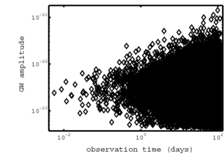
Figure 10: The simulated BBH inspiral population assuming a local rate density of $0.3\hskip 1.42262pt\mathrm{Myr}^{-1}\hskip 1.42262pt\mathrm{Mpc}^{-3}$ for 4 months of data, corresponding to 527,680 events. Note how the GW amplitudes incorporate both higher and lower magnitude extremes as observation time increases – corresponding to smaller and larger $z$.

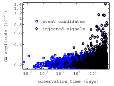
Figure 11: The candidate population of BBH for 4 months of observation time – around 37,000 events – represented by grey squares. Of these candidates, the 2173 events that correspond to injected signals are shown as black diamonds. The remainder are classed as false alarms.

Figure 12 shows the PEH population of BBH events extracted from one 4-month data segment. Each point represents the maximum amplitude of events observed as a function of observation time. Also shown is the BBH inspiral amplitude PEH of Fig. 5 and the Gaussian noise amplitude PEH threshold, which models the progressive maximum amplitude growth of the Gaussian detector noise used in our simulation (see section 4.2). The small gradient of the noise PEH in comparison with the astrophysical PEH curve highlights the fact that the temporal evolution of the Gaussian detector noise, highly dependent on the sampling frequency, is much slower, a result of the low probability of events in the tail of the distribution (Coward et al., 2005). Similarly, the narrower 90% threshold for the Gaussian-noise PEH is also a result of tighter constraints on the amplitude distribution for the Gaussian noise model.

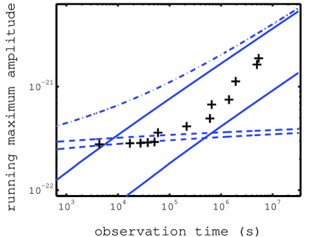
Figure 12: The PEH population of BBH for 4 months of observation time at advanced LIGO sensitivity are shown by crosses, with the solid lines representing the associated 90% amplitude PEH thresholds (see Fig 5). In addition, we show the 90% Gaussian noise amplitude PEH curves (dashed lines), which illustrate the temporal amplitude evolution of Gaussian detector noise. The dot-dashed line represents the absolute amplitude upper limit at 95% confidence for signal + noise.

For early observation times ($\lesssim$ 30,000 s) the PEH population is dominated by false alarms, lying close to the Gaussian noise PEH. As observation time increases, the astrophysical PEH population begins to dominate. An additional threshold, shown by the dot-dashed line, is constructed by combining the null-PEH curves from both populations. This threshold is the 95% amplitude upper limit for our BBH inspiral PEH population – this curve represents the result of obtaining maximum amplitudes for both the noise and sources.

6 The Log N - Log A distribution

We now want to determine the key astrophysical parameter, the source local rate density $r_{0}$, from data such as that presented in the previous section. First we will consider the conventional method of determining source rate densities based on the brightness distribution of sources. This will allow us to quantify the effectiveness of the PEH in determining the local rate density of BBH events. The log N–log P source count distribution (Guetta et al., 2005; Totani, 1999; Schmidt, 2001) is the number of events $N(>\hskip 1.42262ptP)$, of luminosity $L$ and peak flux $P$, within a maximum redshift, $z_{\mathrm{max}}(L,P_{\mathrm{lim}})$, recorded by a detector of flux limit $P_{\mathrm{lim}}$. Such a distribution can be fitted to a predicted log N–log P curve to obtain rate estimates or to constrain the luminosity function.

For our standard-candle GW population, we convert peak flux to a maximum GW amplitude, $A$, yielding a log N–log A distribution of the form:

$$N(>A)=\int_{0}^{z(L,A)}\tau_{\mathrm{0}}\frac{\mathrm{d}R}{\mathrm{d}z}\mathrm{d}z\,$$ (15)

where $\tau_{\mathrm{0}}$ represents the observation time and the differential event rate, $\mathrm{d}R/\mathrm{d}z$, is given by equation 1. In comparison with the log N–log P distribution, which has a gradient of $-3/2$ under a Euclidean geometry, the log N–log A has a slope of $-3$. The curve includes a noise component which approximates the average contribution from detector noise and is scaled by a factor 0.4, the mean value of the antenna response function for a single GW detector (Finn, 1993). By fitting to 100 synthetic data sets, we find these approximations introduce a systematic error of $\pm 6\%$ to the final estimates.

To fit the candidate event population, $E$, against the log N–log A curve, we consider two scenarios: firstly an idealized case, in which the detector has correctly resolved all the injected events in $E$; secondly a suboptimum case, in which the data consists of both injected signals and false alarms. To implement the first scenario we eliminate any false alarms by including only event triggers that correspond to injected signals. For the second scenario we use the whole candidate population of event triggers and false alarms. In section 8 we will apply the PEH method to both scenarios, thereby allowing a direct comparison.

Data stream	SFR model	Estimate of $r_{0}$
		(in units of $\tilde{r}_{0}$)
1	SF2	$1.00\pm 0.07$
1	constant	$1.74\pm 0.11$
1	SF1	$0.99\pm 0.07$
1	SH	$1.46\pm 0.10$
2	SF2	$1.01\pm 0.07$
2	constant	$1.67\pm 0.10$
2	SF1	$0.99\pm 0.07$
2	SH	$1.48\pm 0.10$

Table 1: The results of least squares fitting to the log N – log A distributions of two independent data steams, each representing 4 months of observation time. The data consists of 2273 events for data steam 1 and 2173 events for data stream 2. The results for data stream 1 are shown in Fig 13. The data streams represent the output of a perfect detector – all false alarms have been dismissed. The SFR model is the one used in the fit; the estimated ranges of $r_{0}$ are given at 90% confidence.

Data stream	SFR model	Estimate of $r_{0}$
		(in units of $\tilde{r}_{0}$)
1	SF2	$1.36\pm 0.08$
1	constant	$1.96\pm 0.13$
1	SF1	$1.35\pm 0.08$
1	SH	$1.80\pm 0.12$
2	SF2	$1.28\pm 0.08$
2	constant	$1.86\pm 0.13$
2	SF1	$1.27\pm 0.08$
2	SH	$1.77\pm 0.13$

Table 2: The same as for Table 1, but for data with a high false alarm rate. The data consists of 38241 events for data stream 1 and 37873 events for data stream 2. The results for data stream 1 are shown in Fig 14.

Figure 13 shows the results of fitting against an idealized data set. For data streams 1 and 2 we obtain estimates of $(1.00\pm 0.07)\tilde{r}_{0}$ and $(1.01\pm 0.07)\tilde{r}_{0}$ within 90% confidence using a non-linear regression model based on SF2, the model used to simulate our data. Table 1 shows that the estimates obtained using fits based on four different SFR models recover the true rate to within an average of 46%. These estimates represent the upper limits obtainable by applying the log N – log A method to our simulated data set. We note that the choice of SFR model introduces a bias in our estimates of $r_{0}$. These biases result from the SFR model dependence of the all-sky event rate, $R(z)$, as illustrated in Figure 3.

Figure 14 highlights the effect of false alarms on the data sample. At low amplitude, the distribution is augmented by the noise transients resulting in overestimates of the local rate density. We therefore use a thresholding procedure to dismiss all events below log A = -21.55. Using a fit based on the SF2 model, we obtain estimates of $(1.36\pm 0.08)\tilde{r}_{0}$ using data stream 1 and $(1.28\pm 0.08)\tilde{r}_{0}$ for data stream 2. The estimates obtained using fits based on the four different SFR models are shown in Table 2. The consistency of each pair shows that the statistical errors are small. In addition to the biases resulting from the different SFR models used, for this suboptimum case there is a significant bias due to the effect of false alarms in the distribution. In comparison, one might expect the PEH method, which considers only the most energetic events as a function of time, should be less sensitive to false alarms due to noise, but may have less precision since not all events are utilized. This is considered in the analysis below.

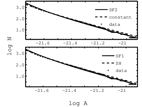
Figure 13: A least squares fit to simulated linear-linear GW data, using predicted brightness distributions based on different SFR models, with a single free parameter, $r_{0}$. The data are candidate events from an event population that correspond to injected signals – this represents an idealized data set, in which we assume all false alarms have been dismissed by the detector. The top panel shows the result of fits based on SF2 and a constant (non-evolving) model; the bottom panel shows fits based on SF1 and SH. The estimates obtained using this fitting procedure are given in Table 1.

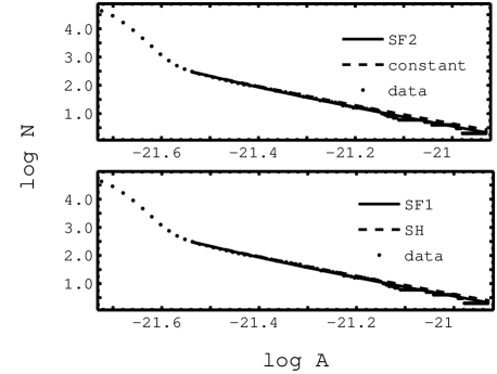
Figure 14: The non-linear regression models of Fig. 13, are fitted to the full candidate population, consisting of both injected events and false alarms. We fit to the data above a threshold of log A = -21.55. The estimates obtained using this fitting procedure are given in Table 2.

7 Fitting to the PEH population

The dependence of the PEH on $r_{0}$, as demonstrated in Fig. 4, provides a means of fitting the PEH curves to a candidate PEH population, $C$, and estimating $r_{0}$. However, an obstacle to this procedure is highlighted in Fig. 12, which shows that $C$ is dominated by detector noise at early observation times ($t$ $\lesssim$ 30,000 s). This reduces the samples available to fit to the amplitude PEH curves.

To reduce the inclusion of false alarms in the fitting procedure, we only include the sample of $C$ above 30,000 s. This threshold corresponds to the change in gradient of the PEH distribution as injected events become dominant over the Gaussian noise components at long observation times (see Fig. 12). This choice of threshold will vary for different astrophysical populations, depending on the emission energies and rates. After applying this threshold, we expect a total PEH population, $C$, of about 7 – 11 events for four months of observation time. We can compensate for any loss of events by this thresholding procedure, by utilizing the signature of the PEH to increase our sample space as discussed below.

Test	Subset	Sample space of	KS Probability
	combination	test samples	$P(>Z_{\mathrm{n}})$
1	1 $\times$ 4 month	8, 8	0.36
2	2 $\times$ 2 month	10, 11	0.59
3	3 $\times$ 1.3 month	17, 18	0.74
4	4 $\times$ 1 month	22, 21	0.81

Table 3: The results obtained from 2D Kolmogorov-Smirnov tests between two 4-month samples of BBH data, extracted from the same simulated data stream. Each sample is split into different numbers of subsets of equal duration and recombined to increase the sample size. We see that the KS statistic improves with sample space for these combinations.

We can increase the sample space of $C$ by splitting our candidate event population, $E$, into $l$ subsets of equal observation time. By applying the PEH filter to each subset and recombining, we form a more highly populated sample $\widetilde{C}$ – the temporal duration of which will now correspond to the length of each individual subset.

The available subset configurations are given by $S_{i},\hskip 1.42262pti=1,...,l$. As the PEH is independent of when the detector is switched on, the PEH signature imprinted within each subset, $S_{i}$, will be set by the subset’s duration. When we combine all $S_{\mathrm{i}}$, to form $\widetilde{C}$, the individual signatures will be subsequently imprinted within the overall sample space. This useful procedure enables us to increase the statistical sample.

When splitting and recombining $C$, there is a delicate balance between improving the statistics by increasing the sample space, and reducing it by decreasing the duration. The most efficient way to increase the population of $C$, whilst retaining the embedded statistical signature of the PEH can be determined using a two-dimensional Kolmogorov-Smirnov test (Fasano & Franceschini, 1987). This test determines the probability of two sets being drawn from the same population distribution.

We calculated the two-dimensional Kolmogorov-Smirnov probabilities $P^{\mathrm{KS}}$ obtained using two consecutive 4-month samples taken from the same simulated data stream. A high value of $P^{\mathrm{KS}}$ will provide evidence of the statistical compatibility of two samples. Table 3 shows that a KS probability of 81% was obtained by splitting the data into four 1-month subsets and recombining. We therefore use this configuration to produce $\widetilde{C}$, the PEH data to which we will apply our fitting procedure.

It should be noted however, that the best choice of $l$, corresponding to the sample configuration with the strongest statistical PEH signature, may vary for different candidate event populations, $E$, depending on the observation time. For example, in performing the same test on three months of data we found that a larger $P^{\mathrm{KS}}$ was obtained using $l=3$ than for $l=4$ – the result of a loss in the PEH signature for samples of shorter temporal duration. For this paper, to illustrate the PEH technique and avoid any additional complications, we maximize the sample space by using a 4-month sample of data.

To constrain the local rate density we apply a least-squares fit to the candidate population $\widetilde{C}$ using an amplitude PEH curve as a linear regression model with free parameter $r_{0}$. When equation 6 is fitted to the data it is necessary to determine the value of $\epsilon$ that correctly estimates $r_{0}$. This value, equal to 0.36, was experimentally verified by fitting to 1000 synthetic data sets using $\epsilon$ as the only free parameter.

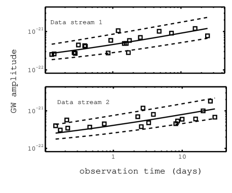
Figure 15: A least squares fit to simulated GW data using a 36% PEH curve based on SF2 as a non-linear regression model. The data correspond to an idealized situation in which all false alarms have been dismissed. Using a PEH fit based on SF2 we obtain an estimate of $(1.26\pm 0.56)\tilde{r}_{0}$ for data stream 1 and $(0.84\pm 0.53)\tilde{r}_{0}$ for the data stream 2. As an additional test of the PEH model, the dashed lines show that the 90% PEH thresholds are a good fit to the data.

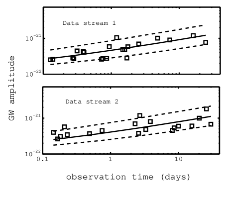
Figure 16: The same fitting function as used in Figure 15 is applied to data which include both injected events and false alarms. We obtain an estimate of $(1.43\pm 0.61)\tilde{r}_{0}$ for data stream 1 and $(0.83\pm 0.51)\tilde{r}_{0}$ for the data stream 2. We again fit the 90% PEH thresholds to the data, shown by the dashed lines.

8 RESULTS

Data stream	SFR model	Events	Estimate of $r_{0}$
			(in units of $\tilde{r}_{0}$)
1	SF2	19	$1.26\pm 0.56$
1	constant	19	$1.43\pm 0.63$
1	SF1	19	$1.25\pm 0.56$
1	SH	19	$1.37\pm 0.60$
2	SF2	18	$0.84\pm 0.53$
2	constant	18	$0.94\pm 0.57$
2	SF1	18	$0.83\pm 0.52$
2	SH	18	$0.92\pm 0.56$

Table 4: The results of least squares fitting to the PEH distributions of two independent data steams, each representing 4 months of observation time. The data represents that of an idealized situation in which all false alarms have been dismissed. A PEH fit to data stream 1 is shown in Fig 15. The SFR model is the one used in the fitting function. The numbers of events used in each fit are shown along with the estimates of $r_{0}$ given at 90% confidence.

Data stream	SFR model	Events	Estimate of $r_{0}$
			(in units of $\tilde{r}_{0}$)
1	SF2	21	$1.43\pm 0.61$
1	constant	21	$1.61\pm 0.71$
1	SF1	21	$1.42\pm 0.63$
1	SH	21	$1.55\pm 0.69$
2	SF2	19	$0.83\pm 0.51$
2	constant	19	$0.94\pm 0.55$
2	SF1	19	$0.82\pm 0.51$
2	SH	19	$0.91\pm 0.54$

Table 5: The same as for Table 1, but for data with a high false alarm rate. A PEH fit to data stream 1 is shown in Fig 16.

In this section we present the results obtained by least-squares fitting to candidate PEH populations $\widetilde{C}$ using the 36% amplitude PEH curve as a linear regression model with free parameter $r_{0}$. We use the same two sets of data as in section 5 and consider again two different scenarios: firstly, an idealized case in which the detector operates at high efficiency and has correctly dismissed all false alarms, and secondly, a suboptimum case in which data include false alarms.

Figure 15 shows the results of a non-linear fit to both data streams for the idealized case in which all false alarms have been dismissed. This fit uses a PEH curve based on SF2, the model used to generate the data, as a non-linear regression model and yields estimates of $(1.26\pm 0.56)\tilde{r}_{0}$ for data stream 1 and $(0.84\pm 0.53)\tilde{r}_{0}$ for data stream 2. As an additional test of the PEH model, this figure shows that the data is well constrained by the 90% amplitude PEH thresholds.

Estimates of $r_{0}$ obtained using PEH curves based on all SFR models are shown in Table 4. We see that we obtain mean estimates to within around a factor of 1.5 for data streams 1 and 2. As a result of the smaller data set used in the PEH fitting procedure, estimates can be sensitive to the distribution of data. This effect is highlighted in Figure 15 which shows that the PEH distribution of data stream 1 tends towards the upper PEH threshold, producing higher estimates of $r_{0}$.

The uncertainties in these estimates are greater than those obtained using the brightness distribution. For example, using a fit based on SF2, the brightness distribution recovered the true rate within 7% and 8% for data streams 1 and 2, while the equivalent estimates obtained using the PEH fit were within 82% and 69%. We note however, that the results obtained using the PEH method are not as prominently effected by bias due to different SFR models as those obtained using a brightness distribution.

In Figure 16 we see the result of a least-squares fit to data which contains both the injected events and false alarms. The numerical estimates determined by applying the PEH fitting procedure to these data are presented in Table 5 for both data streams 1 and 2. The mean estimates for both data streams are within a factor of 1.5 of the true value of $r_{0}$.

To determine the effect of false alarms on our estimates it is useful to eliminate the effects of using different SFR models in our fitting procedures. This can be best achieved by looking at the results obtained using SF2, the model used to produce the candidate data streams. We see that a PEH fit based on SF2 yields estimates of $(1.43\pm 0.61)\tilde{r}_{0}$ for data stream 1 and $(0.83\pm 0.51)\tilde{r}_{0}$ for data stream 2. We see that the inclusion of false alarms has resulted in a 24% and a 3% decrease in accuracy for data streams 1 and 2 respectively. In comparison, estimates using an SF2 model to fit to the brightness distribution degraded by up to 44% for data stream 1 and 35% for data stream 2.

These results imply that the PEH method is less prone to errors due to the inclusion of false alarms. This outcome arises because the PEH distribution is composed of the most energetic events as a function of observation time, thereby omitting most false alarms. We note however that the PEH method has a lower resolution than that of the brightness distribution – a direct result of the smaller data sets used in the fitting procedure. This obvious disadvantage will be discussed in the next section.

Tables 6 and 7 show the estimates obtained by combining brightness distribution and PEH data. When compared to the results obtained using the brightness distribution in Tables 1 and 2, we see that including the PEH data improves the estimates by at least 1-2% in most cases. In addition, these results indicate that the PEH method can be employed as an additional test of consistency.

Data stream	SFR model	Estimate of $r_{0}$
		(in units of $\tilde{r}_{0}$
1	SF2	$1.00\pm 0.06$
1	constant	$1.73\pm 0.10$
1	SF1	$0.99\pm 0.06$
1	SH	$1.45\pm 0.09$
2	SF2	$1.00\pm 0.06$
2	constant	$1.64\pm 0.09$
2	SF1	$0.98\pm 0.06$
2	SH	$1.46\pm 0.09$

Table 6: The constraints on the true local rate density, $r_{0}$, obtained by combining the results of least squares fitting to the log N – log A distributions (Table 1) and the PEH distributions (Table 4) of the two independent data steams. The data sets represent the output of a perfect detector – all false alarms have been dismissed. As previously, the SFR model is the one used in the fit; the estimated ranges of $r_{0}$ are given at 90% confidence.

Data stream	SFR model	Estimate of $r_{0}$
		(in units of $\tilde{r}_{0}$)
1	SF2	$1.36\pm 0.07$
1	constant	$1.94\pm 0.12$
1	SF1	$1.35\pm 0.07$
1	SH	$1.79\pm 0.11$
2	SF2	$1.26\pm 0.07$
2	constant	$1.81\pm 0.12$
2	SF1	$1.25\pm 0.07$
2	SH	$1.72\pm 0.12$

Table 7: The same as for Table 6, but this time we combine the estimates of Tables 2 and 5 for data with a high false alarm rate.

9 Conclusions

We have shown that the PEH filter allows an independent estimate of the rate density of BBH coalescence events detected by advanced GW detectors. The main results and their limitations are summarized below:

1. For a candidate population of BBH with Galactic inspiral rate ${\cal R}_{\rm gal}^{BBH}\sim 30\hskip 2.84526pt\mathrm{Myr}^{-1}$, a fit to 4 months of interferometer data was sufficient to obtain estimates of $r_{0}$ to within a factor of 2 at the 90% confidence level.

   By applying both brightness distribution and PEH methods to data streams with a high false alarm rate we find that the brightness distribution method is the more accurate if the detector is operating at high efficiency. For the case in which the data contains a large proportion of false alarms, we find the PEH fit gives less bias. This is because this method naturally suppresses low-amplitude false-alarms. Of the two methods, the PEH method has lower resolution due to the fact that fewer events contribute to the data. The overall performance of the PEH filter suggests that it is accurate enough to be considered as an additional tool to determine event rate densities, particularly if the detector is operating at low efficiency. A combination of the PEH and brightness distribution methods provides two independent estimates of $r_{0}$. The combination of both estimates provides a self consistent test and also increases the overall precision of the rate estimates.
   

2. One disadvantage of the PEH filter, in comparison with fitting to the amplitude distribution, is that it uses only a small sample of the overall data set. We are investigating techniques to increase the sample size. Initial results suggest that applying the PEH filter in both temporal directions can increase the overall PEH population and improve the resolution and accuracy of the estimates. This technique will be particularly useful in data sets in which a large event occurs after a comparatively short observation time.
   

3. We note that the value for reference local rate density, $\tilde{r}_{0}$, obtained from the population synthesis calculations of Belczynski et al. (2002), is at the upper end of predictions. We plan to investigate the performance of the PEH method for lower values of $\tilde{r}_{0}$ for which we expect a smaller number of events in the PEH distribution. Initial calculations suggest that an order of magnitude decrease in $\tilde{r}_{0}$ will result in a PEH population of around 7 – 11 events for a 4-month data set rather than the 15 – 22 events expected for $\tilde{r}_{0}$ used in this study. As discussed previously, techniques in which we can increase the PEH sample will be of great importance for astrophysical populations with lower rate densities.
   

4. For the noise levels considered in this study, the PEH fits are only weakly affected by the inclusion of false alarms, but estimates using a brightness distribution are shown to degrade. This implies that the PEH method may be most effective when applied to data output from signals that are not well modelled, such as transient burst sources, for which we expect a substantial number of false alarms to be present. Recent developments in the modelling of GW emissions from core-collapse supernova (SNe) suggest that the detectable background population of such sources may be numerous enough to apply the PEH technique (Ott et al., 2006).
   

5. The PEH filter, by definition includes the temporal distribution of the sources, hence provides a means of predicting the energies of future events.
   

6. Our results show that at the detector sensitivity assumed here, the value of $r_{0}$ cannot be separated from evolution effects, so that different SFR curves create bias in the estimated value of $r_{0}$. For larger spans of data and more sensitive detectors such as EURO (Sathyaprakash, 2004) it may be possible to fit the PEH data or the brightness distribution to determine the entire function $R(z)$.

References

- Abbott et al. (2005) Abbott B. et al., 2005, Phys. Rev. D, 72, 062001
- Abbott et al. (2004) Abbott B. et al., 2004, Phys. Rev. D, 69, 122001
- Abramovici et al. (1992) Abramovici A. et al., 1992, Nature, 5055, 325
- Ando (1999) Ando S., 2004, Journal of Cosmology and Astroparticle Physics, 0406, 7
- Arnaud et al. (2003a) Arnaud N., Barsuglia M., Bizouard M-A., Brisson V., Cavalier F., Davier M., Hello P., Kreckelbergh S., Porter E. K., 2003a, Phys. Rev. D, 68, 102001
- Arnaud et al. (2003b) Arnaud N., Barsuglia M., Bizouard M-A., Brisson V., Cavalier F., Davier M., Hello P., Kreckelbergh S., Porter E. K., Pradier T., 2003b, Phys. Rev. D, 67, 062004
- Arnaud et al. (2002) Arnaud N., Barsuglia M., Bizouard M-A., Canitrot P., Cavalier F., Davier M., Hello P., Pradier T., 2002, Phys. Rev. D, 65, 042004
- Baker et al. (2002) Baker J., Campanelli M., Lousto C.O., Takahashi R., 2005, Phys. Rev. D, 65, 124012
- Belczynski et al. (2002) Belczynski K., Kalogera V., Bulik T., 2002, ApJ, 572, 407
- Bizouard et al. (2003) Bizouard M-A., Arnaud N., Barsuglia M.,Brisson V., Cavalier F., Davier M., Hello P., Kreckelbergh S., Porter E. K., Pradier T., 2003, Class. Quantum Grav. 20, S829
- Bulik et al. (2004a) Bulik T., Gondek-Rosinska D., Belczynski K., 2004a, MNRAS, 352, 1372
- Bulik et al. (2004b) Bulik T., Belczynski K., Rudak B., 2004b, A&A, 415, 417
- Bulik & Belczynski (2003) Bulik T., Belczynski K., 2003, ApJ, 589, L37
- Burgay et al. (2003) Burgay M. et al., 2003, Nature, 426, 531
- Burger et al. (2005) Burger E. et al., 2005, Nature, 438, 988
- Chernoff & Finn (2003) Chernoff D. F., Finn L. S., 1993, ApJ, 411, L5
- Coward (2005) Coward D. M., 2005, MNRAS, 360, L77
- Coward & Burman (2005) Coward D., Burman R., 2005, MNRAS, 361, 362
- Coward et al. (2005) Coward D. M., Lilley M., Howell E. J., Burman R.R. and Blair D. G., 2005, MNRAS, 364, 807
- Cutler and Thorne (2002) Cutler C., Thorne K. S., 2002, in Proceedings of the 16th International Conference on General Relativity and Gravitation, edited by N.T Bishop and S. N. Maharaj (Singapore: World Scientific).
- Fasano & Franceschini (1987) Fasano G., Franceschini A., 1987, MNRAS, 225, 155
- Finn (2001) Finn L. S., 2001, Phys. Rev. D, 63, 102001
- Finn (1993) Finn L. S., Chernoff D. F., 1993, Phys. Rev. D, 47, 6
- Flanagan & Hughes (1998) Flanagan É. É., Hughes S. A., 1998, Phys. Rev. D, 57, 8
- Guetta et al. (2005) Guetta D., Piran T., Waxman E., 2005, ApJ, 619, 412
- Jaranowski et al. (1998) Jaranowski P., Królak A., Schultz B. F., 1998, Phys. Rev. D, 58, 063001
- Kalogera et al. (2001) Kalogera V., Narayan R., Spergel D. N., Taylor J. H., 2001, ApJ, 556, 340
- Kalogera et al. (2004) Kalogera et al., 2004, ApJ, 601, L179
- Maggiore (2000) Maggiore M., 2000, Physics Reports, 331, 6
- Miller et al. (2004) Miller M., Gressman P., Suen W-M, 2004,1, Phys. Rev. D, 69, 064026
- Ott et al. (2006) Ott C. D., Burrows A., Dessart L., Livne E., 2005,1, Phys. Rev. Lett, 96, 201102
- Peebles (1993) Peebles P. J. E., 1993, Principles of Physical Cosmology, Princeton Univ. Press, Princeton NJ
- Phinney (1991) Phinney E. S., 1991, ApJ, 380, L17
- Porciani & Madau (2001) Porciani C., Madau P., 2001, ApJ, 548, 522
- Pradier et al. (2001) Pradier T., Arnaud N., Bizouard M-A., Cavalier F., Davier M., Hello P. , 2001, Phys. Rev. D, 63, 042002
- Sathyaprakash (2004) Sathyaprakash B. S., 2004, gr-qc 0405136
- Schmidt (2001) Schmidt M., 2001, ApJ, 552, 36
- Schutz (1986) Schutz B. F., 1986, Nature, 323, 310
- Shawhan & Ochsner (2004) Shawhan P. and Ochsner E., 2004, Class. Quantum Grav, 21, S1757
- Springel and Hernquist (2003) Springel V., Hernquist L., 2003, MNRAS, 339, 312
- Thorne (1995) Thorne K. S. in Gravitational waves from compact objects in Proceedings of IAU Symoposium 165, Compact Stars in Binaries, eds. J. van Paradijs, E. van den Heuvel and E. Kuulkers, Publisher, Kluwer Academic Publishers, 1995
- Totani (1999) Totani T., 1999, ApJ, 511, 41