Visual/infrared interferometry of Orion Trapezium stars: Preliminary dynamical orbit and aperture synthesis imaging of the $\theta^{1}$Orionis C system

Abstract

Context. Located in the Orion Trapezium cluster, $\theta^{1}$Ori C is one of the youngest and nearest high-mass stars (O5-O7) and known to be a close binary.

Aims. By tracing its orbital motion, we aim to determine the orbit and dynamical mass of the system, yielding a characterization of the individual components and, ultimately, also new constraints for stellar evolution models in the high-mass regime.

Methods. Using new multi-epoch visual and near-infrared bispectrum speckle interferometric observations obtained at the BTA 6 m telescope, and IOTA near-infrared long-baseline interferometry, we traced the orbital motion of the $\theta^{1}$Ori C components over the interval 1997.8 to 2005.9, covering a significant arc of the orbit. Besides fitting the relative position and the flux ratio, we applied aperture synthesis techniques to our IOTA data to reconstruct a model-independent image of the $\theta^{1}$Ori C binary system.

Results. The orbital solutions suggest a highly eccentricity ($e\approx 0.91$) and short-period ($P\approx 10.9$ yrs) orbit. As the current astrometric data only allows rather weak constraints on the total dynamical mass, we present the two best-fit orbits. Of these two, the one implying a system mass of $48\leavevmode\nobreak\ M_{\sun}$ and a distance of 434 pc to the Trapezium cluster can be favored. When also taking the measured flux ratio and the derived location in the HR-diagram into account, we find good agreement for all observables, assuming a spectral type of O5.5 for $\theta^{1}$Ori C1 ($M=34.0\leavevmode\nobreak\ M_{\sun}$, $T_{\rm eff}=39\,900$ K) and O9.5 for C2 ($M=15.5\leavevmode\nobreak\ M_{\sun}$, $T_{\rm eff}=31\,900$ K). Using IOTA, we also obtained first interferometric observations on $\theta^{1}$Ori D, finding some evidence for a resolved structure, maybe by a faint, close companion.

Conclusions. We find indications that the companion C2 is massive itself, which makes it likely that its contribution to the intense UV radiation field of the Trapezium cluster is non-negligible. Furthermore, the high eccentricity of the preliminary orbit solution predicts a very small physical separation during periastron passage ($\sim 1.5$ AU, next passage around 2007.5), suggesting strong wind-wind interaction between the two O stars.

1 Introduction

Stellar mass is the most fundamental parameter, determining, together with the chemical composition and the angular momentum, the entire evolution of a given star. Stellar evolutionary models connect these fundamental parameters with more easily accessible, but also highly uncertain observables such as the luminosity and the stellar temperature. Particularly towards the pre-main-sequence (PMS) phase and towards the extreme stellar masses (i.e. the low- and high-mass domain), the existing stellar evolutionary models are still highly uncertain and require further empirical verification through direct and unbiased mass estimates, such as those provided by the dynamical masses accessible in binary systems. Recently, several studies were able to provide dynamical masses for low-mass PMS stars (e.g.  Tamazian et al. 2002; Schaefer et al. 2003; Boden et al. 2005), while direct mass measurements for young O-type stars are still lacking.

Furthermore, in contrast to the birth of low-mass stars, the formation mechanism of high-mass stars is still poorly understood. In particular, the remarkably high binary frequency measured for young high-mass stars might indicate that the way high-mass stars are born differs significantly from the mass accretion scenario via circumstellar disks, which is well-established for low- and intermediate-mass stars. For instance, studies conducted at the nearest high-mass star-forming region, the Orion Nebular Cluster (ONC, at a distance of $440\pm 34$ pc, Jeffries 2007), revealed 1.1 companions per primary (for high-mass stars $M>10M_{\sun}$,  Preibisch et al. 1999), which is significantly higher than the mean number of companions for intermediate and low-mass stars.

In the very center of the ONC, four OB stars form the Orion Trapezium; three of which ($\theta^{1}$Ori A, B, C) are known to be multiple (Weigelt et al. 1999; Schertl et al. 2003). $\theta^{1}$Ori D (alias HD 37023, HR 1896, Parenago 1889) has no confirmed companion, although a preliminary analysis of the radial velocity by Vitrichenko (2002a) suggests that it might be a spectroscopic binary with a period of $\sim 20$ or $40$ days.

A particularly intruiging young ($<1$ Myr, Hillenbrand 1997) high-mass star in the Trapezium cluster is $\theta^{1}$Ori C (alias 41 Ori C, HD 37022, HR 1895, Parenago 1891). $\theta^{1}$Ori C is the brightest source within the ONC and also the main source of the UV radiation ionizing the proplyds and the M42 H ii region. A close ($33$ mas) companion with a near-infrared flux ratio of $\sim 0.3$ between the primary ($\theta^{1}$Ori C1) and the secondary ($\theta^{1}$Ori C2) was discovered in 1997 using bispectrum speckle interferometry (Weigelt et al. 1999). Donati et al. (2002) estimated the mass of $\theta^{1}$Ori C to be $44\pm 5M_{\sun}$, making it the most massive star in the cluster. The same authors give an effective temperature of $45\,000\pm 1\,000$ K and a stellar radius of $8.2\pm 1.1\leavevmode\nobreak\ R_{\sun}$. Simón-Díaz et al. (2006) estimated the mass independently using evolutionary tracks and by performing a quantitative analysis of $\theta^{1}$Ori C spectra and obtained $M_{\rm evol}=33M_{\sun}$ and $M_{\rm spec}=45\pm 16M_{\sun}$, respectively. Long series of optical and UV spectroscopic observations revealed that the intensity and also some line profiles vary in a strictly periodic way. With $15.422\pm 0.002$ days, the shortest period was reported by Stahl et al. (1993). Several authors interpret this periodicity, which in the meantime was also detected in X-ray (Gagne et al. 1997), within an oblique magnetic rotator model, identifying 15.422 d with the rotation period of the star. Stahl et al. (1996) detected a steady increase in radial velocity, confirmed by Donati et al. in 2002, which suggests a spectroscopic binary with an orbital period of at least 8 years. Vitrichenko (2002b) searched for long-term periodicity in the radial velocity and reported two additional periods of 66 days and 120 years, which he interpreted as the presence of, in total, three components in the system.

Given the unknown orbit of the speckle companion, it still must be determined which one of these periods corresponds to the orbital motion of C2. Since the discovery of C2 in 1997, three measurements performed with bispectrum speckle interferometry showed that the companion indeed undertakes orbital motion (Schertl et al. 2003), reaching the largest separation of the two components in autumn 1999 with $43\pm 2$ mas. In order to follow the orbital motion, we monitored the system using infrared and visual bispectrum speckle interferometry and in 2005, for the first time, also using infrared long-baseline interferometry.

An interesting aspect of the dynamical history of the ONC was presented by Tan (2004). He proposed that the Becklin-Neugebauer (BN) object, which is located 45″ northwest of the Trapezium stars, might be a runaway B star ejected from the $\theta^{1}$Ori C multiple system approximately $4\,000$ yrs ago. This scenario is based on proper motion measurements, which show that BN and $\theta^{1}$Ori C recoil roughly in opposite directions, and by the detection of X-ray emission potentially tracing a wind bow shock. Three-body interaction is a crucial part of this interpretation, and C2 is currently the only candidate which could have been involved. Therefore, a high-precision orbit measurement of C2 might offer the unique possibility to recover the dynamical details of this recent stellar ejection. However, another study (Rodríguez et al. 2005) also aimed to identify the multiple system from which BN was ejected and identified Source I as the likely progenitor system. Later, Gómez et al. (2005) added further evidence to this interpretation by identifying Source $n$ as a potential third member of the decayed system.

2 Observations and Data Reduction

Table 1: Observation Log.

Target	Instrument	Date	Filtera	Detectorb	No. Interferograms	Calibratorsd
	and Configuration	[UT]		and Modec	Target/Calibrator
$\theta^{1}$Ori C	BTA 6m/Speckle	1997.784	$H$	P/DIT=150 ms	519/641	$\theta^{1}$Ori D
$\theta^{1}$Ori C	BTA 6m/Speckle	1998.838	$K^{\prime}$	H/DIT=120 ms	438/265	$\theta^{1}$Ori D
$\theta^{1}$Ori C	BTA 6m/Speckle	1999.737	$J$	H/DIT=100 ms	516/244	$\theta^{1}$Ori D
$\theta^{1}$Ori C	BTA 6m/Speckle	1999.8189	$G^{\prime}$	S/DIT=5 ms	500/–	–
$\theta^{1}$Ori C	BTA 6m/Speckle	2000.8734	$V^{\prime}$	S/DIT=5 ms	1 000/–	–
$\theta^{1}$Ori C	BTA 6m/Speckle	2001.184	$J$	H/DIT=80 ms	684/1 523	$\theta^{1}$Ori D
$\theta^{1}$Ori C	BTA 6m/Speckle	2003.8	$J$	H/DIT=160 ms	312/424	$\theta^{1}$Ori D
$\theta^{1}$Ori C	BTA 6m/Speckle	2003.9254	$V^{\prime}$	S/DIT=2.5 ms	1 500/–	–
$\theta^{1}$Ori C	BTA 6m/Speckle	2003.928	$V^{\prime}$	S/DIT=2.5 ms	2 000/–	–
$\theta^{1}$Ori C	BTA 6m/Speckle	2004.8216	$V^{\prime}$	S/DIT=5 ms	2 000/–	–
$\theta^{1}$Ori C	BTA 6m/Speckle	2006.8	$V^{\prime}$, $R^{\prime}$	–	–	–
$\theta^{1}$Ori C	IOTA A35-B15-C0	2005 Dec 04	$H$	1L7R, 2L7R	11 400/8 050	HD 14129, HD 36134, HD 34137,
						HD 50281, HD 63838
$\theta^{1}$Ori C	IOTA A35-B15-C10	2005 Dec 02	$H$	2L7R, 4L7R	4 400/4 950	HD 34137, HD 50281, HD 63838
$\theta^{1}$Ori C	IOTA A35-B15-C10	2005 Dec 03	$H$	2L7R	4 600/2 450	HD 28322
$\theta^{1}$Ori C	IOTA A35-B15-C15	2005 Dec 01	$H$	2L7R, 4L7R	7 250/5 000	HD 20791, HD 34137, HD 36134
$\theta^{1}$Ori C	IOTA A25-B15-C0	2005 Dec 06	$H$	2L7R, 4L7R	5 250/4 875	HD 28322, HD 34137, HD 36134,
						HD 74794
$\theta^{1}$Ori D	IOTA A35-B15-C0	2005 Dec 04	$H$	2L7R	800/2 800	HD 14129, HD 36134, HD 34137,
						HD 50281, HD 63838
$\theta^{1}$Ori D	IOTA A25-B15-C0	2005 Dec 06	$H$	2L7R, 4L7R	1 800/4 875	HD 28322, HD 34137, HD 36134,
						HD 74794

Notes – ^a) Filter central wavelength and bandwidth, in nm ($\lambda_{c}$/$\Delta\lambda$) – $V^{\prime}$: 545/30; $G^{\prime}$: 610/20; $R^{\prime}$: 800/60; $J$: 1 239/138; $H$: 1 613/304; $K^{\prime}$: 2 115/214.

^b) P: PICNIC detector, H: HAWAII array, S: Multialkali S25 intensifier photocathode

^c) For the IOTA measurements, we used different detector read modes to adapt to the changing atmospheric conditions. The two numbers in the given 4-digit code denote the value of the loop and read parameter (Pedretti et al. 2004) of the PICNIC camera. Since data taken in different readout modes is calibrated independently, the scattering between the data sets also resembles the typical calibration errors (see Figure 4).

^d) The dash symbol in the calibrator column indicates speckle measurements for which no calibrator was observed.

Table 2: IOTA Calibrator Stars Information

Star	V	H	Spectral	Adopted UD diameter
			Type	[mas]
HD 14129	5.5	3.3	G8.5III	$1.01\pm 0.01$a
HD 20791	5.7	3.5	G8.5III	$0.89\pm 0.01$a
HD 28322	6.2	3.9	G9III	$0.82\pm 0.01$a
HD 34137	7.2	4.4	K2III	$0.80\pm 0.01$a
HD 36134	5.8	3.2	K1III	$1.16\pm 0.02$a
HD 50281	6.6	4.3	K3V	$0.77\pm 0.10$b
HD 63838	6.4	3.6	K2III	$0.95\pm 0.01$a
HD 74794	5.7	3.5	K0III	$1.07\pm 0.01$a

Notes – ^a UD diameter taken from the CHARM2 catalog (Richichi et al. 2005).

^b UD diameter taken from getCal tool (http://mscweb.ipac.caltech.edu/gcWeb/gcWeb.jsp).

2.1 Bispectrum speckle interferometry

Speckle interferometric methods are powerful techniques for overcoming the atmospheric perturbations and for reaching the diffraction-limited resolution of ground-based telescopes, both at near-infrared and visual wavelengths. Since the discovery of $\theta^{1}$Ori C2 in 1997, we have monitored the system with the Big Telescope Alt-azimuthal (BTA) 6.0 m telescope of the Special Astrophysical Observatory located on Mt. Pastukhov in Russia. For the speckle observations at visual wavelengths, a $1280\times 1024$ pixel CCD with a multialkali S25 intensifier photocathode was used. The near-infrared speckle observations were carried out using one 512$\times$512 pixel quadrant of the Rockwell HAWAII array in our speckle camera, with pixel sizes of 13.4 mas ($J$-band), 20.2 mas ($H$-band), and 27 mas ($K$-band) on the sky.

For the speckle observations at infrared wavelengths, we recorded interferograms of $\theta^{1}$Ori C and of the nearby unresolved star $\theta^{1}$Ori D in order to compensate for the atmospheric speckle transfer function. The number of interferograms and the detector integration times (DITs) are listed in Table 1.

The modulus of the Fourier transform of the object (visibility) was obtained with the speckle interferometry method (Labeyrie 1970). For image reconstruction we used the bispectrum speckle interferometry method (Weigelt 1977, Weigelt & Wirnitzer 1983, Lohmann et al. 1983, Hofmann & Weigelt 1986).

2.2 IOTA long-baseline interferometry

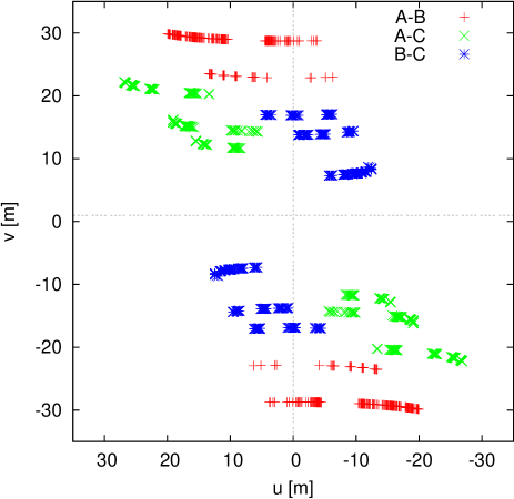
Figure 1: $uv$-plane coverage obtained on $\theta^{1}$Ori C with the four IOTA array configurations used. The relatively strong asymmetry in the $uv$-plane coverage mainly results from the position of $\theta^{1}$Ori C relatively close to the celestrial equator.

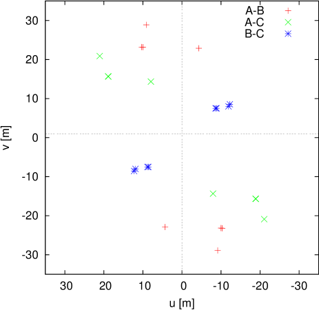
Figure 2: $uv$-plane coverage obtained on $\theta^{1}$Ori D with two IOTA array configurations. Symbols and colors as in Figure 1.

The Infrared Optical Telescope Array (IOTA) is a three-telescope, long-baseline interferometer located at the Fred Lawrence Whipple Observatory on Mount Hopkins, Arizona, operating at visual and near-infrared wavelengths (Traub et al. 2003). Its three 45 cm primary Cassegrain telescopes can be mounted on stations along an L-shaped track, reaching 15 m towards a southeastern and 35 m towards a northeastern direction. After passing a tip-tilt system, which compensates the atmospherically induced motion of the image, and path-compensating delay lines, the three beams are fed into fibers and coupled pairwise onto the IONIC3 integrated optics beam combiner (Berger et al. 2003). The interferograms are recorded by temporal modulation around zero optical path delay (OPD). During data acquisition, a fringe tracker software (Pedretti et al. 2005) continuously compensates potential OPD drifts. This allows us to measure the three interferograms nearly simultaneously within the atmospheric coherence time, preserving the valuable closure phase (CP) information.

For our IOTA observations, we used four different array configurations (see Table 1), obtaining the $uv$-coverage shown in Figure 1. $\theta^{1}$Ori D was observed on two different array configurations, as shown in Figure 2. During each night, we systematically alternated between the target star and calibrators in order to determine the transfer function of the instrument. For more details about the calibrator stars and the number of recorded Michelson interferograms, refer to Table 2.

In order to extract visibilities and CPs from the recorded IOTA interferograms, we used the IDRS data reduction software. Basic principles of the algorithms implemented in this software package were already presented in Kraus et al. (2005), although several details have been refined to obtain optimal results for fainter sources as well, such as those observed in this study.

To estimate the fringe amplitude (visibility squared, $V^{2}$), we compute the continuous wavelet transform (CWT), which decomposes the signal into the OPD-scale domain, providing scale (frequency) resolution while preserving the information about the fringe OPD. The turbulent Earth atmosphere introduces fast-changing OPD variations between the combined telescopes (also known as atmospheric piston), degenerating the recorded interferograms. By measuring the extension of the fringe packet in the CWT along both the scale and the OPD axis, we identify the scans which are most affected by this effect and reject them from further processing. For the remaining scans, we apply a method similar to the procedure presented by Kervella et al. (2004). First, the fringe peak is localized in the CWT. In order to minimize noise contributions, a small window around the fringe peak position is cut out. Then we integrate along the OPD axis, yielding a power spectrum. After recentering the fringe peak position for each scan (to compensate frequency changes induced by atmospheric piston), we average the power spectra for all scans within a dataset. In the resulting averaged power spectrum, we fit and remove the background contributions and integrate over the fringe power to obtain an estimate for $V^{2}$.

Another refinement in our software concerns the CP estimation. We found that the best signal-to-noise ratio (SNR) can be achieved by averaging the bispectra from all scans. The bispectrum is given by the triple product of the Fourier transform of the scans at the three baselines (Hofmann & Weigelt 1993). Then, we use the triple amplitude to select the bispectrum elements with the highest SNR and average the triple phases of these elements in the complex plane to obtain the average closure phase.

3 Aperture synthesis imaging

$\begin{array}[]{ccc}\textnormal{{\bf 1999.7}, BTA, $J$-band}&\textnormal{{\bf 2004.8}, BTA, $V^{\prime}$-band}&\textnormal{{\bf 2005.9}, IOTA, $H$-band}\\[-31.29802pt] \includegraphics[width=207.7052pt]{6965fig3a.ps}&\includegraphics[width=207.7052pt]{6965fig3b.ps}&\includegraphics[width=207.7052pt]{6965fig3c.ps}\\[-59.75078pt] \includegraphics[width=207.7052pt]{6965fig3d.ps}&\includegraphics[width=207.7052pt]{6965fig3e.ps}&\includegraphics[width=207.7052pt]{6965fig3f.ps}\end{array}$

Figure 3: Left, Middle: Bispectrum speckle $J$ and $V^{\prime}$-band images reconstructed from BTA-data. Right: Aperture synthesis image of $\theta^{1}$Ori C reconstructed from our IOTA $H$-band data. Besides the false-color representation in the upper row, we show the images below as contours with the best-fitted positions marked with star symbols (see Table 3). In the image in the lower right corner, the restoring beam for the IOTA aperture synthesis image is shown as an inset. Over the six year interval covered by the images, orbital motion is clearly conceivable (1999/2004/2005: $\rho$=43/24/14 mas; $\Theta$=214°/191°/163°).

Interpreting optical long-baseline interferometric data often requires a priori knowledge about the expected source brightness distribution. This knowledge is used to choose an astrophysically motivated model whose parameters are fitted to the measured interferometric observables (as applied in Sect. 4).

However, the measurement of CPs allows a much more intuitive approach; namely, the direct reconstruction of an aperture synthesis image. Due to the rather small number of telescopes combined in the current generation of optical interferometric arrays, direct image reconstruction is limited to objects with a rather simple source geometry; in particular, multiple systems (for images reconstructed from IOTA data, see Monnier et al. 2004; Kraus et al. 2005).

Using our software based on the Building Block Mapping algorithm (Hofmann & Weigelt 1993), we reconstructed an aperture synthesis image of the $\theta^{1}$Ori C system from the data collected during our IOTA run. Starting from an initial single delta-function, this algorithm builds up the image iteratively by adding components in order to minimize the least-square distance between the measured bispectrum and the bispectrum of the reconstructed image.

The resulting image is shown in Figure 3 and provides a model-independent representation of our data. By combining the data collected during six nights, we make the reasonable assumption that the orbital motion over this interval is negligible.

The clean beam, which we used for convolution to obtain the final image, is rather elliptical (see inset in Figure 3), representing the asymmetries in the $uv$-coverage.

4 Model fitting

4.1 Binary model fitting for $\theta^{1}$Ori C

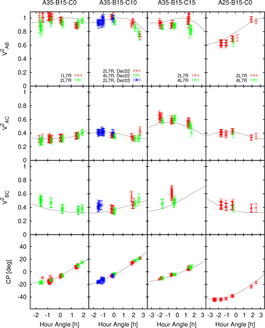
Figure 4: Visibilities and Closure Phases derived from the recorded IOTA interferograms for $\theta^{1}$Ori C as a function of hour angle (points with error bars). The solid line shows the binary model fit, described in more detail in Section 4. The different symbols represent the different detector modes used (see Table 1). The data for each detector mode was calibrated separately, so the scattering of the data groups represents the typical calibration errors.

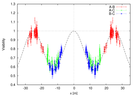
Figure 5: Projection of the sampled Fourier plane along the fitted binary PA of $162.74\degr$ ($x=u\cos\Theta-v\sin\Theta$), clearly revealing the binary signature. The dashed line shows the theoretical cosine visibility profile for a binary star with separation 13.55 mas and intensity ratio 0.28.

Table 3: Relative astrometry and photometry for the $\theta^{1}$Ori C binary system

							(O–C) Orbit #1			(O–C) Orbit #2
Telescope	Date	Filter	Flux ratio	$\Theta^{a}$	$\rho$	Ref.	$\Theta$	$\rho$		$\Theta$	$\rho$
			$F_{\rm C2}/F_{\rm C1}$	[°]	[mas]		[°]	[mas]		[°]	[mas]
BTA 6m/Speckle	1997.784	H	$0.26\pm 0.02$	$226.0\pm 3$	$33\pm 2$	b	+3.0	+0.0		+3.0	+0.5
BTA 6m/Speckle	1998.838	K’	$0.32\pm 0.03$	$222.0\pm 5$	$37\pm 4$	b	+3.8	-2.6		+3.8	-2.5
BTA 6m/Speckle	1999.737	J	$0.31\pm 0.02$	$214.0\pm 2$	$43\pm 1$	c	-0.9	+1.5		-0.9	+1.5
BTA 6m/Speckle	1999.8189	G’	$0.35\pm 0.04$	$213.5\pm 2$	$42\pm 1$	–	-1.1	+0.5		-1.1	+0.5
BTA 6m/Speckle	2000.8734	V’	$0.35\pm 0.03$	$210.0\pm 2$	$40\pm 1$	–	-0.8	-0.8		-0.9	-0.8
BTA 6m/Speckle	2001.184	J	$0.29\pm 0.02$	$208.0\pm 2$	$38\pm 1$	c	-1.6	-2.1		-1.7	-2.1
BTA 6m/Speckle	2003.8	J	$0.30\pm 0.02$	$199.3\pm 2$	$29\pm 2$	–	+3.9	+0.5		+2.8	+0.5
BTA 6m/Speckle	2003.9254	V’	–	$199.0\pm 2$	$29\pm 2$	–	+3.6	+1.3		+3.4	+1.3
BTA 6m/Speckle	2003.928	V’	–	$199.1\pm 2$	$29\pm 2$	–	+3.8	+1.3		+3.6	+1.3
BTA 6m/Speckle	2004.8216	V’	$0.34\pm 0.04$	$190.5\pm 4$	$24\pm 4$	–	+4.2	+2.4		+4.0	+2.4
IOTA	2005.92055	H	$0.28\pm 0.03$	$162.74\pm 2$	$13.55\pm 0.5$	–	-0.5	+0.0		-1.0	+0.0
BTA 6m/Speckle	2006.8	V’, R	–	–	$<15$	–	–	–		–	–

Notes – ^a) Following the convention, we measure the position angle (PA) from north to east.

References – ^b) Weigelt et al. 1999, ^c) Schertl et al. 2003

Although the aperture synthesis image presented in the last section might also be used to extract parameters like binary separation, orientation, and intensity ratio of the components ($I_{\rm C2}/I_{\rm C1}=0.26$, $\rho=14.1$ mas, $\Theta=162$°), more precise values, including error estimates, can be obtained by fitting the measured visibilities and CPs to an analytical binary model.

The applied model is based on equations 7–12 presented in Kraus et al. (2005) and uses the least-square Levenberg-Marquardt method to determine the best-fit binary separation vector and intensity ratio. In order to avoid potential local minima, we vary the initial values for the least-square fit on a grid, searching for the global minimum.

Since the apparent stellar diameter of $\theta^{1}$Ori C is expected to be only $\sim 0.2$ mas at the distance of Orion, for our fits we assume that both stellar components appear practically unresolved to the IOTA baselines. Furthermore, we assume that the relative position of the components did not change significantly over the 6 nights of observation.

Figure 4 shows the measured IOTA visibilities and CPs and the observables corresponding to our best-fit binary model ($\chi^{2}_{V^{2}}/\textnormal{dof}=1.35$, $\chi^{2}_{CP}/\textnormal{dof}=1.48$). The separation $\rho$, PA $\Theta$, and intensity ratio of this binary model are given in Table 3, together with the positions derived from the speckle observations. To illustrate more clearly that the measured IOTA visibilities resemble a binary signature, in Figure 5 we show a projection of the sampled two-dimensional Fourier plane along the binary vector, revealing the cosine modulation corresponding to the Fourier transform of a binary brightness distribution.

For the speckle data (providing a complete Fourier sampling up to the spatial frequency corresponding to the diameter of the telescope primary mirror), we determine the binary parameters by fitting a two-dimensional cosine function directly to the 2-D speckle interferogram power spectrum.

4.2 Resolved structure around $\theta^{1}$Ori D:
Potential detection of a companion

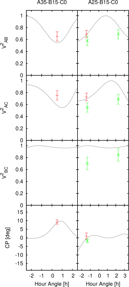
Figure 6: Visibilities and Closure Phases derived from the recorded IOTA interferograms for $\theta^{1}$Ori D (points with error bars). The solid line shows the binary model fit, described in more detail in Section 4.2.

Besides the main target of our observational programme, $\theta^{1}$Ori C, during the two nights with the best seeing conditions, we also recorded four datasets on $\theta^{1}$Ori D. Despite lower flux ($\theta^{1}$Ori D: $H$=5.9, $\theta^{1}$Ori C: $H$=4.6), the quality of the derived visibilities and CPs seems reliable, although slightly larger errors must be assumed. $\theta^{1}$Ori D appears resolved in our measurements with a significant non-zero CPs signal ($\sim 10$°) on the A35-B15-C0 baseline. This CP indicates deviations from point-symmetry, as expected for a binary star. We applied the binary model fit described in Sect. 4.1 and found the binary system with an intensity ratio of 0.14, $\rho=18.4$ mas, and $\Theta=41$° (Figure 6) to be the best-fit model ($\chi^{2}/\textnormal{dof}=1.36$).

However, considering the $uv$-coverage of the existing dataset, this solution is likely not unique, and it can not be ruled out that other geometries, such as for inclined circumstellar disk geometries with pronounced emission from the rim at the dust sublimation radius (see e.g.  Monnier et al. 2006), might also produce the asymmetry required to fit the data.

5 Results

5.1 Preliminary physical orbit of the $\theta^{1}$Ori C binary system

Figure 7: Top: Two best-fit apparent orbits of the $\theta^{1}$Ori C binary system (solid and dashed line). Each position measurement (see Table 3) is connected to its predicted position with an $O$–$C$ line. Besides our orbital solutions (see Table 4), the line of nodes and the predicted positions for the interval 2007.0 to 2008.5 (increments of 0.25 yrs) are shown. North is up and east is to the left. Bottom: Radial velocity variations of both components computed for our orbital solutions using the method presented by Pourbaix (1998). For the mass ratio $M_{\rm C2}/M_{\rm C1}$, we assume 0.47, as obtained from our modeling of the flux ratio presented in Sect. 5.4. When computing the radial velocity curve, the (unknown) system velocity $V_{0}$ represents a free-parameter corresponding to a velocity offset, which we set to $-5$ km s^-1 for this plot. The radial velocity measurements (points with errorbars) were taken from Vitrichenko (2002b).

Table 4: Preliminary orbital solutions, dynamical parallaxes, and system masses for $\theta^{1}$Ori C.

		Orbit #1	Orbit #2
$P$	[yrs]	10.98	10.85
$T$		1996.52	1996.64
$e$		0.909	0.925
$a$	[mas]	41.3	45.0
$i$	[°]	105.2	103.7
$\Omega$	[°]	56.5	56.9
$\omega$	[°]	65.7	68.2
$\chi^{2}/\textnormal{dof}$		1.61	1.59
$\pi_{\rm dyn}$a)	[mas]	$2.304\pm 0.066$	$2.585\pm 0.074$
$d_{\rm dyn}$a)	[pc]	$434\pm 12$	$387\pm 11$
$(M_{\rm C1}+M_{\rm C2})$a)	[$M_{\sun}$]	$47.8\pm 4.2$	$44.8\pm 3.9$

Notes – ^a) The errors on the dynamical parallaxes and corresponding distances were estimated by varying the measured binary flux ratio within the observational uncertainties, the assumed spectral types for the bolometric correction by one sub-class, the extinction by $\pm 0.2$ magnitudes, and by using three different MLRs (by Baize & Romani 1946; Heintz 1978; Demircan & Kahraman 1991). However, the given errors do not reflect the uncertainties on the orbital elements $a$ and $P$. Due to the presence of the multiple orbital solutions, it is currently not possible to quantify these errors reliably.

Table 5: Ephemerides for the $\theta^{1}$Ori C orbital solutions presented in Table 4

Epoch	Orbit #1			Orbit #2
	$\Theta$	$\rho$		$\Theta$	$\rho$
	[°]	[mas]		[°]	[mas]
2007.0	100.9	8.7		101.8	8.7
2007.5	28.6	1.9		-22.4	0.8
2008.0	229.1	21.7		227.9	23.0
2008.5	224.6	30.1		223.8	31.0
2009.0	221.7	35.1		221.1	35.8
2010.0	217.5	40.2		217.0	40.5
2011.0	213.9	41.6		213.4	41.6
2012.0	210.3	40.5		209.8	40.2
2013.0	206.3	37.5		205.8	37.0
2014.0	201.4	33.0		200.8	32.3
2015.0	194.6	27.1		193.7	26.3
2016.0	183.4	20.1		181.7	19.2
2017.0	159.7	12.8		155.1	12.0

Our multi-epoch position measurements of the $\theta^{1}$Ori C system can be used to derive a preliminary dynamical orbit. To find orbital solutions, we used the method described by Docobo (1985). This method generates a class of Keplerian orbits passing through three base points. From this class of possible solutions, those orbits are selected which best agree with the measured positions, where we use the error bars of the individual measurements as weight. In order to avoid over-weighting the orbit points which were sampled with several measurements at similar epochs (two measurements in 1999.7-1999.8 and three measurements in 2003.8-2003.9), we treated each of these clusters as single measurements.

In Table 4 we give the orbital elements corresponding to the two best orbital solutions found. As the $\chi^{2}/\textnormal{dof}$ values of the two presented orbits are practically identical, the existing astrometric data does not allow us to distinguish between these solutions. These orbits and the corresponding O–C vectors are shown in Figure 7 (see Table 3 for a list of the O–C values). As the ephemerids in Table 5 and also the position predictions (dots) in Figure 7 show, future high-accuracy long-baseline interferometric measurements are needed to distinguish between these orbital solutions.

Potentially, additional constraints on the $\theta^{1}$Ori C binary orbit could be provided by radial velocity measurements, such as those published by Vitrichenko (2002b) and in the references therein. However, the complexity of the $\theta^{1}$Ori C spectrum – including the line variability corresponding to the magnetically confined wind-shock region expected towards $\theta^{1}$Ori C – makes both the measurement and the interpretation of radial velocities for $\theta^{1}$Ori C very challenging. Since it is unclear whether these velocities really correspond to the orbital motion of the binary system or perhaps to variations in the stellar wind from $\theta^{1}$Ori C, we did not include these velocity measurements as a tough constraint in the final orbital fit, but show them together with the radial velocities corresponding to our best-fit orbit solutions in Figure 7.

Both orbital solutions suggest that during periastron passage, the physical separation between C1 and C2 decreases to $\sim 1.5$ AU, corresponding to just $\sim 30$ stellar radii. Besides the strong dynamical friction at work during such a close passage, strong wind-wind interaction can also be expected.

It is worth mentioning that besides the presented best-fit orbital solutions, a large number of solutions with longer orbital periods exist, which are also fairly consistent with the astrometric measurements. However, since these orbits have slightly higher $\chi^{2}/\textnormal{dof}$ values than the solutions presented above and also correspond to physically unreasonable masses ($M_{\rm C1}\leavevmode\nobreak\ +\leavevmode\nobreak\ M_{\rm C2}\leavevmode\nobreak\ \lesssim\leavevmode\nobreak\ 20$ or $\gtrsim 130\leavevmode\nobreak\ M_{\sun}$, assuming $d$=440 pc), we rejected these formal solutions.

5.2 Dynamical masses and parallaxes

Kepler’s third law relates the major axis $a$ and the orbital period $P$ with the product of the system mass and the cube of the parallax; i.e. $(M_{\rm C1}+M_{\rm C2})\cdot\pi^{3}=a^{3}/P^{2}$ (where $a$ and $\pi$ are given in mas, $P$ in years, and $M$ in solar masses).

In order to separate the system mass and the parallax in absence of spectroscopic orbital elements, the method by Baize & Romani (1946) can be applied. This method assumes that the component masses follow a mass-luminosity relation (MLR), which, together with a bolometric correction and extinction-corrected magnitudes, allows one to solve for the system mass $M_{\rm C1}+M_{\rm C2}$ and the dynamical parallax $\pi_{\rm dyn}$. When using the MLR by Demircan & Kahraman (1991), the bolometric correction for O5.5 and O9.5 stars by Martins et al. (2005), and the extinction corrected magnitudes given in Table 6, we derive the dynamical masses and parallaxes given in Table 4. When comparing the distances corresponding to the dynamical parallaxes derived for Orbit #1 ($d_{\rm dyn}=\pi^{-1}_{\rm dyn}=434$ pc) and Orbit #2 ($d_{\rm dyn}=387$ pc) with distance estimates from the literature (e.g. $d=440\pm 34$ pc from Jeffries 2007; see also references herein), orbit solution #1 appears much more likely. The dynamical system mass corresponding to Orbit #1 is $47.8\leavevmode\nobreak\ M_{\sun}$, which must be scaled by a factor $(d/d_{\rm dyn})^{3}$ when distances other than $d_{\rm dyn}=434$ pc are assumed.

5.3 The orbital parameters in the context of reported periodicities

Several studies have already reported the detection of periodicity in the amplitude, width, or velocity of spectral lines around $\theta^{1}$Ori C. This makes it interesting to compare whether one of those periods can be attributed to the presence of companion C2:

$P\approx 15.422\pm 0.002$ d:

By far, the best-established periodicity towards $\theta^{1}$Ori C was detected in hydrogen recombination lines and various photospheric and stellar-wind lines (Stahl et al. 1993, 1996; Walborn & Nichols 1994; Oudmaijer et al. 1997). Later, the same period was also found in the X-ray flux (Gagne et al. 1997) and even in modulations in the Stokes parameters (Wade et al. 2006). Although possible associations with a hypothetical low-mass stellar companion were initially discussed (Stahl et al. 1996), this period is, in the context of the magnetic rotator model, most often associated with the stellar rotation period. We can rule out that C2 is associated with this periodicity, as we do not see significant motion of C2 within the seven days covered by the IOTA measurements.

60 d$\leavevmode\nobreak\ <\leavevmode\nobreak\ P\leavevmode\nobreak\ <\leavevmode\nobreak\ 2$ yrs, $P\approx 120$ yrs:

Vitrichenko (2002b) fitted radial velocity variations assuming the presence of two companions and determined possible periods of $729.6/L$ days (with $L$ an integer $<13$) for the first and $\sim 120$ yrs for the second companion. Since our orbital solutions do not match any of these periods, we consider an association of $\theta^{1}$Ori C2 very unlikely.

$\leavevmode\nobreak\ P\leavevmode\nobreak\ \gtrsim\leavevmode\nobreak\ 8$ yrs:

Stahl (1998) reported a steady increase in radial velocity. Donati et al. (2002) confirmed this trend and estimated that this increase might correspond to the orbital motion of a companion with a period between 8 yrs (for a highly eccentric orbit) and 16 yrs (for a circular orbit). With the found period of $\sim 11$ yrs, it is indeed very tempting to associate $\theta^{1}$Ori C2 with this potential spectroscopic companion. However, as noted in Sect. 5.1, the set of available spectroscopic radial velocity measurements seems rather inhomogeneous and fragmentary and might contain observational biases due to the superposed shorter-period spectroscopic line variations, as noted above.

5.4 Nature of the $\theta^{1}$Ori C components

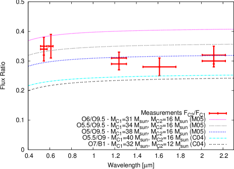
Figure 8: Measured intensity ratio of the $\theta^{1}$Ori C components as a function of wavelength (points with errorbars). For various spectral-type combinations, the curves show the expected intensity ratio, assuming the stars contribute purely photospheric emission (black-body emission with luminosities and effective temperatures as given in the stellar evolution models from Martins et al. (2005, M05) and Claret (2004, C04)).

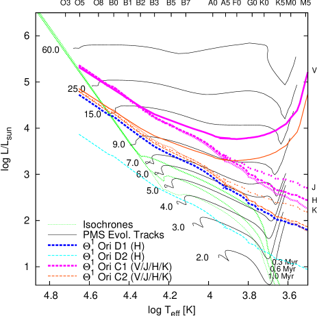
Figure 9: HR-diagram with PMS evolutionary tracks ($Z=0.02$; thin solid lines with the corresponding masses labeled aside). For masses $\leq 7M_{\sun}$ ($\geq 9M_{\sun}$), the tracks from Siess et al. 2000 (Bernasconi & Maeder 1996) were used. The three dotted lines represent the isochrones for 0.3, 0.6, and 1.0 Myr (Bernasconi & Maeder 1996). Using the synthetic colors and bolometric corrections compiled by Kenyon & Hartmann (1995, including data from , , and others) and the O star colors by Martins et al. (2005) and Martins & Plez (2006), we converted the measured photometry for $\theta^{1}$Ori C1, C2, D1, and D2 into the corresponding allowed locations in the HR-diagram (thin red lines).

Table 6: Derived dereddened magnitudes and colors for the $\theta^{1}$Ori C components. For the photometry of the total system, we used data from Hillenbrand et al. (1998, $J$=4.63, $H$=4.48, $K$=4.41) and Hillenbrand (1997, $V$=5.12). An extinction of $A_{V}=1.74$ (Hillenbrand 1997) was assumed (using the reddening law by Mathis 1990 and, similar to Mathis & Wallenhorst 1981, a high $R_{V}=5.0$).

	V	J	H	K	V–J	V–H	V–K	J–H	J–K	H–K
$\theta^{1}$Ori C1	3.70	4.35	4.38	4.49	-0.65	-0.69	-0.80	-0.04	-0.15	-0.11
$\theta^{1}$Ori C2	4.87	5.65	5.81	5.73	-0.78	-0.94	-0.86	-0.15	-0.08	0.07

Most studies which can be found in literature attributed the whole stellar flux of $\theta^{1}$Ori C to a single component and determined a wide range of spectral types including O5.5 (Gagné et al. 2005), O6 (Levato & Abt 1976; Simón-Díaz et al. 2006), O7 (van Altena et al. 1988), to O9 (Trumpler 1931). In order to resolve this uncertainty, it might be of importance to take the presence of $\theta^{1}$Ori C2 into account. Besides the constraints on the dynamical masses derived in Section 5.1, additional information about the spectral types of $\theta^{1}$Ori C1 and C2 can be derived from the flux ratio of the components in the recorded bands.

In contrast to our earlier studies (Weigelt et al. 1999; Schertl et al. 2003), we can now also include the $V$-band flux ratio measurement to constrain the spectral types of the individual components. The $V$-band is of particular interest, as a relative increase of the flux ratio $F_{\rm C2}/F_{\rm C1}$ from the visual to the near-infrared would indicate the presence of circumstellar material, either as near-infrared excess emission or intrinsic extinction towards C2 (assuming similar effective temperatures for both components). Our speckle measurements indicate that $F_{\rm C2}/F_{\rm C1}$ stays rather constant from the visual to the near-infrared. Therefore, in the following we assume that the major contribution of $\theta^{1}$Ori C2 to the measured flux is photospheric.

In Figure 8 we show the measured $F_{\rm C2}/F_{\rm C1}$ as a function of wavelength and compare it to model curves corresponding to various spectral-type combinations for C1 and C2. To compute the model flux ratios, we simulate the stellar photospheric emission as black-body emission $B(T_{\rm eff})$ with effective temperatures $T_{\rm eff}$ and stellar radii $R$, as predicted by stellar evolutionary models (Claret 2004; Martins et al. 2005):

$$\left(\frac{F_{\rm C2}}{F_{\rm C1}}\right)(\lambda)=\frac{B(T_{\rm eff}^{\rm C2})R_{\rm C2}^{2}}{B(T_{\rm eff}^{\rm C1})R_{\rm C1}^{2}}$$ (1)

Under these assumptions, the companion C2 would have to be rather massive ($M_{\rm C2}/M_{\rm C1}=0.45\pm 0.15$) to obtain reasonable agreement with the measured flux ratios (see Figure 8).

Using a value for $A_{V}$ from literature, the flux ratios can also be used to estimate the photometry of the individual components (Table 6). Then, the spectral type of C1 and C2 can be determined by comparing the location of the stars in the HR-diagram with stellar evolution models. For this, we adopt the procedure from Schertl et al. (2003) and convert the derived photometry into locations in the HR-diagram using the colors and bolometric corrections from Kenyon & Hartmann (1995, and references therein) and Martins & Plez (2006). Assuming coevality for both stars, the spectral type of the individual components can be constrained by finding the location where the curves for the various spectral bands and the isochrone intersect. As can be seen in Figure 9, the allowed locations for C1 intersect the Zero-Age Main Sequence (ZAMS) around $T_{\rm eff}=46\,000\pm 4\,000$ K, $\log L/L_{\sun}=5.3\pm 0.2$ (corresponding to O5) and around $T_{\rm eff}=33\,000\pm 2\,000$ K, $\log L/L_{\sun}=4.5\pm 0.1$ (corresponding to O9) for C2.

We conclude that the spectral type combination, which simultaneously provides good agreement to the measured flux ratios, the HR-diagram, and the dynamical masses derived in Sect. 5.1, is given by the following stellar parameters (using the evolutionary models from Martins et al. 2005):
C1: O5.5 ($M=34.0\leavevmode\nobreak\ M_{\sun}$, $T_{\rm eff}=39\,900$ K, $\log L/L_{\sun}=5.41$)
C2: O9.5 ($M=15.5\leavevmode\nobreak\ M_{\sun}$, $T_{\rm eff}=31\,900$ K, $\log L/L_{\sun}=4.68$)

5.5 Nature of the potential $\theta^{1}$Ori D companion

Although the $\theta^{1}$Ori D binary parameters presented in Sect. 4.2 must be considered preliminary, it might be interesting to determine the spectral type of the putative components. We apply the procedure discussed in Sect. 5.4 to determine the photometry of the components from the measured intensity ratio (photometry for the unresolved system from Hillenbrand et al. 1998: $H$=5.84) and derive $H_{D1}$=5.98 and $H_{D2}$=8.12, respectively.

Searching again for the intersection between the allowed locations in the HR-diagram with the isochrones applicable to the ONC (Figure 9), the best agreement for D1 can be found with $T_{\rm eff}=31\,500\pm 4\,000$ K, $\log L/L_{\sun}=4.25\pm 0.1$ (corresponding to O9.5). Accordingly, D2 might be either a B4 or B5 type star which has just reached the ZAMS ($T_{\rm eff}=16\,000\pm 4\,000$ K, $\log L/L_{\sun}=2.6\pm 0.2$) or a pre-main-sequence K0 type star ($T_{\rm eff}=5\,000\pm 1\,000$ K, $\log L/L_{\sun}=1.3\pm 0.2$).

Vitrichenko (2002a) examined radial velocity variations of $\theta^{1}$Ori D and presented preliminary spectroscopic orbital elements for a companion with a 20.2 d period (or twice that period, P=40.5 d). Assuming $20\leavevmode\nobreak\ M_{\sun}$ as the system mass, these periods correspond to a major axis of 0.05 or 0.08 AU ($\sim 0.1$ or $0.2$ mas). Since this is far below the 18 mas suggested by our binary model fit, we do not associate our potential companion with the proposed spectroscopic companion.

The multiplicity rate in a young stellar population such as the Trapezium cluster is an important quantity which might allow us to draw conclusions not only about the dynamical history of the ONC, but also about the mechanisms controlling the star formation process. The detection of a new companion around $\theta^{1}$Ori D further increases the multiplicity rate for high-mass stars in the ONC. For instance, considering the sample of 13 Orion O- and B-type stars studied by Preibisch et al. (1999) now yields 10 visual and 5 spectroscopic detected companions (including one quintuple system, namely $\theta^{1}$Ori B). This corresponds to an average observed companion star frequency (CSF) of 1.15 companions per primary. Despite the fact that this value only represents a strict lower limit due to observational incompleteness, it is already higher than the incompleteness-corrected CSF determined by Duquennoy & Mayor (1991) for a distance-limited sample of solar-type field stars (0.5 companions per primary). Köhler et al. (2006) have reported that the CSF for low- and intermediate-mass stars in the ONC is about a factor of 2.3 lower than the CSF in the Duquennoy & Mayor sample, making the differences in the CSF between the low-, intermediate-, and high-mass star population in the ONC highly significant. Several studies (e.g.  Preibisch et al. 1999; Bally & Zinnecker 2005; Bonnell & Bate 2005) have already interpreted this as evidence that different formation mechanisms (e.g. stellar coalescence vs. accretion) might be at work in different mass regimes.

6 Conclusions

We have presented new bispectrum speckle interferometric and infrared long-baseline interferometric observations of the Orion Trapezium stars $\theta^{1}$Ori C and D. This data was used to reconstruct diffraction-limited NIR and visual speckle images of the $\theta^{1}$Ori C binary system and, to our knowledge, the first model-independent, long-baseline aperture-synthesis image of a young star at infrared wavelengths.

For $\theta^{1}$Ori D, we find some indications that the system was resolved by the IOTA interferometer. Although the non-zero closure phase signal suggests asymmetries in the brightness distribution (maybe indicative of a close companion star), further observations are required to confirm this finding.

From our multi-epoch observations on $\theta^{1}$Ori C (covering the interval 1997.8 to 2005.8), we derived the relative position of the companions using model-fitting techniques, clearly tracing orbital motion. We presented two preliminary orbital solutions, of which one can be favoured due to theoretical arguments. This solution implies a period of 10.98 yrs, a semi-major axis of 41.3 mas, a total system mass of $\sim 48M_{\sun}$, and a distance of 434 pc. Furthermore, we find strong indications that $\theta^{1}$Ori C2 will undergo periastron passage in mid 2007. As the binary separation at periastron is expected to be $\sim 1$ mas, further long-baseline interferometric observations on $\theta^{1}$Ori C are urgently needed to refine the orbital elements, the stellar masses, and orbital parallaxes. Through comparison with stellar evolutionary models and modeling of the measured intensity ratio, we find evidence that the companion $\theta^{1}$Ori C2 is more massive ($M_{\rm C2}/M_{\rm C1}\approx 0.45\pm 0.15$) than previously thought; likely of late O (O9/9.5) or early B-type (B0). The contribution of the companion to the total flux of $\theta^{1}$Ori C and the interaction between both stars might be of special importance for a deeper understanding of this intriguing object. Therefore, we strongly encourage observers to acquire high dispersion spectra of the system in order to trace the expected radial velocity variations and the wind-wind interaction of the system.