GRB060218: A Relativistic Supernova Shock Breakout

Abstract

We show that the prompt and afterglow X-ray emission of GRB060218, as well as its early ($t\lesssim 1$ d) optical-UV emission, can be explained by a model in which a radiation- mediated shock propagates through a compact progenitor star into a dense wind. The prompt thermal X-ray emission is produced in this model as the mildly relativistic shock, $\beta\approx 0.85$ carrying few $\times 10^{49}$ erg, reaches the wind (Thomson) photosphere, where the post-shock thermal radiation is released and the shock becomes collisionless. Adopting this interpretation of the thermal X-ray emission, a subsequent X-ray afterglow is predicted, due to synchrotron emission and inverse-Compton scattering of SN UV photons by electrons accelerated in the collisionless shock. Early optical-UV emission is also predicted, due to the cooling of the outer $\delta M\sim 10^{-3}M_{\odot}$ envelope of the star, which was heated to high temperature during shock passage. The observed X-ray afterglow and the early optical-UV emission are both consistent with those expected in this model. Detailed analysis of the early optical-UV emission may provide detailed constraints on the density distribution near the stellar surface.

1. Introduction

In our previous paper (Campana et al., 2006) the points mentioned in the abstract were outlined only briefly, using order-of-magnitude arguments and with very little explanation, due to space limitations. Here we present a more detailed explanation and analysis of the prompt thermal X-ray emission and X-ray afterglow, as well as a calculation of the early optical-UV emission, and show that some claims made in recent publications (Ghisellini et al., 2006; Fan et al., 2006; Li, 2006), according to which the observations are inconsistent with the massive wind interpretation, are not valid.

GRB060218 was unique mainly in two respects: it showed a strong thermal X-ray emission accompanying the prompt non-thermal emission, and a strong optical-UV emission at early, $t\lesssim 1$ d, time. We show here that these features, as well as the X-ray afterglow, can all be explained by a model in which a radiation mediated shock propagates through a compact progenitor star into a massive wind. We have shown in a separate paper (Wang et al., 2006) that the prompt non-thermal X-ray emission can also be explained by this model.

As detailed below, the prompt thermal X-ray emission can be explained as shock breakout at a radius of $\sim 5\times 10^{12}$ cm, which requires a Thomson optical depth (of the plasma ahead of the shock) of $\tau\approx 1$. Breakout may occur at $\sim 5\times 10^{12}$ cm if this is the stellar progenitor radius. However, since the progenitor is likely to be smaller, we suggested the possibility of it being surrounded by an optically thick wind. Another possibility is a pre-explosion ejection of a small mass, $\sim 10^{-6}M_{\odot}$, shell. Here we shall adopt the wind interpretation, since it allows one to explain also the X-ray afterglow. So far, no other quantitative physical models have been worked out for the thermal X-ray emission, nor for the X-ray afterglow. Soderberg et al. (2006) and Fan et al. (2006) have suggested that the afterglow X-ray emission is due to extended activity of the source, for which there is no model or explanation. Ghisellini et al. (2006) suggest, for explaining the X-ray afterglow, an ansatz consisting of the ad-hoc existence of electrons with some prescribed energy distribution, which is different at different times to account for the observations, without a model for the dynamics of the plasma or for the electron energy distribution.

We note that the radio afterglow of GRB060218 discussed by Soderberg et al. (2006) is difficult to explain within the context of the current model. Indeed, as pointed out by Soderberg et al. (2006) and by Fan et al. (2006), it is difficult to explain the radio afterglow and the X-ray afterglow of GRB060218 as due to emission from a single shock wave. These authors have thus chosen to construct models that account for the radio emission only, attributing the X-ray afterglow to a continued activity of the source of an unexplained nature, and not accounting for the prompt X-ray emission and for the early optical-UV emission. We adopt a different approach, showing that the prompt (thermal and non-thermal) X-ray emission, the early optical-UV emission, and the late X-ray afterglow can all be explained within the context of the same model. We argue that it is the radio afterglow, rather than all the other components, which remains unexplained, and which should be attributed to a different component. Since the radio emission carries only a negligible fraction of the energy, and given the large anisotropy of the explosion, it is not difficult to imagine the existence of such an additional low energy component.

In § 2 we discuss the observations and our model. In § 3 we compare our analysis with those of other authors. Our results and conclusions are discussed in § 4.

2. Observations and Model

2.1. Thermal X-ray Emission: Shock Breakout

Possibly the most distinguishing feature of GRB060218 is the strong thermal X-ray emission accompanying the prompt non-thermal emission. The temperature of the thermal X-ray photons observed up to $3\times 10^{3}$ s is $T\approx 0.17$ keV (Campana et al., 2006). The integrated flux of the black-body X-ray component, $6\times 10^{-6}{\rm erg/cm^{2}}$ (see figure 1), corresponds (using $d=145$ Mpc and after correcting for the flux that falls outside the XRT band) to a thermal X-ray energy of $E_{\rm th}\approx 2\times 10^{49}$ erg. This is only an approximate estimate, and the total thermal energy may be somewhat larger, due to the gap in XRT observations between $3\times 10^{3}$ s and $6\times 10^{3}$ s. We consider here a model where this radiation is due to a “shock breakout”.

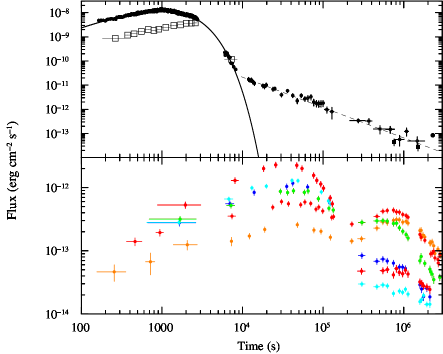
Figure 1.— Upper panel: the X-ray light curve (0.3–10 keV). Open black circles mark Swift-XRT data, filled squares Chandra data (Soderberg et al. 2006) and filled circle XMM-Newton data (de Luca & Marshall 2006). Open squares denote the black body component. A smooth-burst with exponential decay fits the prompt part (solid line). A power law decay with index -1.25 well describes the afterglow tail (dashed line). Count rate-to-flux conversion factors were derived from time-dependent spectral analysis. The X–ray light curve has a long, slow power-law rise followed by an exponential (or steep power-law) decay. At about 10,000 s the light curve breaks to a shallower power-law decay with index $-1.2\pm 0.1$. Lower panel: the UVOT light curve. Filled circles of different colors (on-line version) represent different UVOT filters (from bottom to top between $104-105$ s): $V$ (centered at 544 nm); $B$ (439 nm), $U$ (345 nm), UVW1 (251 nm); UVM1 (217 nm) and UVW2 (188 nm). Specific fluxes have been multiplied by their FWHM widths (75, 98, 88, 70, 51 and 76 nm, respectively).

Supernova (SN) shock waves become radiation-mediated when propagating through the stellar envelope (see Woosley & Weaver, 1986, for review). The energy density behind the shock is dominated by radiation, and the mechanism that converts kinetic energy to thermal energy at the shock transition is Compton scattering. The optical depth of the shock transition layer is $\tau_{s}\simeq c/v_{s}$, where $v_{s}$ is the shock velocity. This thickness is determined by the requirement that the time it takes a fluid element to flow through the transition layer, $\sim\Delta_{s}/v_{s}$, should be comparable to the diffusion time of photons across this layer, $\simeq\tau_{s}\Delta_{s}/c$. As the shock propagates outward, the (Thomson) optical depth of the plasma lying ahead of the shock decreases, and when this optical depth becomes comparable to $\tau_{s}$, Compton scattering can no longer maintain the shock. At this point, radiation escapes ahead of the shock, producing the shock breakout flash (Colgate, 1974; Klein & Chevalier, 1978; Ensman & Burrows, 1992; Matzner & McKee, 1999), and the shock becomes collisional (or collisionless, see Waxman & Loeb, 2001).

Hereafter we use the term ”shock breakout” to denote the event of the transition from radiation to collisional (collisionless) shock mediation, accompanied by the emission of radiation. If the optical depth of the wind surrounding the progenitor star is small, shock breakout will take place as the shock approaches the stellar surface. It is for this reason customary to identify shock breakout with the emergence of the shock from the stellar surface. However, if the optical depth of the wind is large, $>\tau_{s}$, breakout would occur once the shock reaches a radius where the wind optical depth drops to $\tau_{s}$.

As argued in Campana et al. (2006), in order to obtain a breakout flash with energy of $E_{\rm th}\simeq 10^{49}$ erg and temperature $T\approx 0.17$ keV, breakout must occur at a radius of $r\sim 5\times 10^{12}$ cm, and the shock must be mildly relativistic (which implies $\tau_{s}\simeq 1$). Since the progenitor star is presumably smaller than this (e.g. if it is a Wolf-Rayet star), a value of $\tau\simeq 1$ at $r\sim 5\times 10^{12}$ cm may be obtained either by assuming that the progenitor is surrounded by a dense wind, or that an outer shell of the star was ejected to this radius prior to the GRB explosion. The mass of the shell required to obtain $\tau_{s}\simeq 1$ is only $\sim 4\pi r^{2}/\kappa\sim 10^{-6}M_{\odot}$, where $\kappa=0.2{\rm g/cm^{2}}$ is the Thomson opacity for ionized He. For the calculation below we adopt a density profile $\rho\propto r^{-2}$, as would be expected for the wind model. The results obtained for the breakout radius, shock velocity and plasma density at this radius are not sensitive, however, to the details of the density profile shape.

We consider therefore a shock wave of velocity $\beta c$ driven into the wind surrounding the progenitor, whose 4-velocity is $u\equiv\gamma\beta$ where $\gamma=(1-\beta^{2})^{-1/2}$ is the Lorentz factor. Let us first derive the energy and temperature of the post-shock radiation. The post-shock temperature $T_{d}$ is related to the post-shock pressure by $aT_{d}^{4}=3p$, and the observed temperature is given by $\gamma_{d}T_{d}$, where $\gamma_{d}=(1-\beta_{d}^{2})^{-1/2}$ and $\beta_{d}c$ is the post-shock plasma velocity ($\beta_{d}<\beta$). For a strong radiation dominated shock $p=fu^{2}\rho c^{2}$, where $\rho$ is the pre-shock density and $f(u)$ is a factor of order unity. As we show below, the shock is required to be mildly relativistic, $u=$ a few, for which we may approximate $f=0.8$ (for $u\gg 1$, $f=2/3$), and $(u_{d}/u)^{2}\approx 0.6$ ($(u_{d}/u)^{2}=1/2$ for $u\gg 1$). This defines the observed temperature, $T$, to be

$$T\simeq 1u^{3/2}(a^{-1}\rho c^{2})^{1/4}$$ (1)

(for $u\gg 1$, the numerical coefficient is $1/2^{1/4}$ instead of 1). The energy carried by the radiation may be estimated by noting that the energy density of the radiation is given, in the observer frame, by $-p+\gamma_{d}^{2}(aT_{d}^{4}+p)=(4u_{d}^{2}+3)p$, and that the thickness of the shocked plasma shell may be approximated as $d=(\beta-\beta_{d})r$, where $r$ is the shock radius. This yields

$$\frac{E_{\rm th}}{4\pi r^{3}\rho c^{2}}=(\beta-\beta_{d})(4u_{d}^{2}+3)\frac{p}{\rho c^{2}}\simeq 0.5u^{2}$$ (2)

(for $u\gg 1$, the numerical coefficient is $2/3$ instead of 0.5).

For a wind density profile, the optical depth of the wind at radius $r$ is simply $\tau(r)=\kappa\rho(r)r$. Expressing the density in terms of $\tau(r)$ and using eqs. (1) and (2) we find that the shock velocity at breakout is

$$u^{2} = \left(\frac{aT^{4}}{\sqrt{2\pi}c^{3}}\right)^{1/7}\left(\frac{\kappa}{\tau}\right)^{3/14}E_{\rm th}^{1/14}$$ (3)

$$= 2.5\left(\frac{T}{0.17\rm keV}\right)^{4/7}E_{\rm th,49}^{1/14},$$

and that breakout occurs at a radius

$$R_{ph} = \left[\frac{E_{\rm th}^{3}}{(2\pi)^{3}aT^{4}c^{4}}\right]^{1/7}\left(\frac{\kappa}{\tau}\right)^{2/7}$$ (4)

$$= 7.8\times 10^{12}\left(\frac{T}{0.17\rm keV}\right)^{-4/7}E_{\rm th,49}^{3/7}\,{\rm cm},$$

where $E_{\rm th}=10^{49}E_{\rm th,49}$ erg and we have used $\kappa=0.2{\rm g/cm^{2}}$ and $\tau=1$ in the numerical evaluations. Note that the results depends only weakly on the exact values of $\kappa$ and $\tau$.

Eqs. (3) and  (4) imply that the breakout of the shock takes place at a radius $\simeq 7.8\times 10^{12}$ cm, and that the shock is mildly relativistic at breakout, $u^{2}=2.5$ i.e. $\beta=0.85$. These results are in agreement with the order of magnitude estimates given in Campana et al. (2006). Since the shock is found to be mildly relativistic, using $\tau=1$ at shock breakout is justified. In order to produce the shock that is driven into the wind, the explosion is thus required to produce a mildly relativistic shell, $\beta=0.8$, with an energy of a few $\times 10^{49}$ erg. This is remarkably similar to the case of GRB980425/SN1998bw, for which the ejection of a shell of energy $10^{49.7}$ erg and velocity $\beta=0.8$ was inferred from X-ray (Waxman, 2004b) and radio (Kulkarni et al., 1998; Waxman & Loeb, 1999; Chevalier & Li, 1999; Waxman, 2004a) observations.

The wind density at the breakout radius, $\rho=1/\kappa r=10^{-12}{\rm g/cm^{3}}$, is also in agreement with our results in Campana et al. (2006). It is straightforward to verify that the energy density is dominated by radiation, $aT^{4}/nT\sim 10^{9}$. For a wind velocity of $\sim 10^{3}{\rm km/s}$ it corresponds to a mass loss rate of few $\times 10^{-4}M_{\odot}/{\rm yr}$. The relevant mass loss here is that occurring within a day or less of the explosion. The data currently available on wind mass losses suggesting ${\dot{M}}\lesssim\hbox{few}\times 10^{-4}M_{\odot}/{\rm yr}$ refer to much longer timescales, for stars well before any explosion (Meynet & Maeder, 2007). Physically, it is however quite plausible that the mass loss increases considerably as the evolution of the core rapidly approaches the final collapse, accompanied by a rapid increase in the luminosity and the envelope expansion rate.

Note that if both the shell and the wind were spherically symmetric, the characteristic timescale would be $R_{ph}/c=260$ s (for the inferred post shock velocity, $\gamma_{d}\beta_{d}=1.2$, the effects of relativistic beaming are not significant), while the observed timescale of the thermal X-ray emission is $\sim 10^{3}$ s (Campana et al., 2006). However, an anisotropic shell ejection is a natural expectation in a core collapse GRB, since strong rotation is a requisite to make the jet (e.g. MacFadyen & Woosley (1999)). Even “normal” core collapse SN simulations show strong rotation-related anisotropy in the expanding gas (e.g. Burrows, et al. (2007)). Thus, the semi-relativistic outer shell ejected is likely to be anisotropic, either due to an anisotropic explosion, or due to being driven by a jet. This, as well as an anisotropic wind profile caused by rotation (Meynet & Maeder, 2007) should lead to significant departures from sphericity in the shock propagation. Anisotropy is in fact a prediction of this model, which is supported by the detection of linear polarization (Gorosabel et al., 2006). In an anisotropic shock, however, the timescale is no longer the naive spherical $r/c$ value, but is rather given by the sideways pattern expansion timescale, which depends on the angular velocity profile of the anisotropic shell (e.g. at larger angles the shock emerges later due a decreasing velocity profile or due to an increasing wind density away from the symmetry axis, etc.).

2.2. X-ray afterglow: Wind-shell interaction

If the wind shock breakout interpretation is adopted, the subsequent interaction of the ejected relativistic shell with the wind is expected to produce an X-ray afterglow (Waxman, 2004b). The electrons accelerated to high energy in the collisionless shock driven into the wind emit X-ray synchrotron radiation, and may also inverse-Compton scatter optical-UV SN photons to the X-ray band.

As the shock wave driven into the wind expands, it heats an increasing amount of mass to a high temperature and the initial energy of the ejected shell is transferred to the shocked wind. The shell begins to decelerate beyond a radius at which the shocked wind energy becomes comparable to the initial shell energy. This occurs at a time (Waxman, 2004b)

$$t_{dec}=0.06\frac{E_{k,49}}{\beta^{3}(\dot{m}/10)}\,{\rm day}.$$ (5)

Here, $E_{k}=10^{49}E_{k,49}$ erg is the kinetic energy of the shell and

$$\dot{m}\equiv\frac{\dot{M}/v_{w}}{10^{-5}(M_{\odot}/{\rm yr})/10^{3}({\rm km/s})}$$ (6)

For the wind density and shell velocity inferred in § 2.1, $\beta=0.85$ and $\dot{m}\gtrsim 10$, $t_{dec}\lesssim 10^{4}$ s. At $t>t_{dec}$ the energy is carried by shocked wind plasma, and is continuously transferred to a larger mass of newly shocked parts of the wind. Thus, the rate at which energy is transferred to accelerated electrons is $\approx\epsilon_{e}E_{k}/t$, where $\epsilon_{e}$ is the fraction of the post-shock thermal energy carried by electrons. If the electrons cool on a time scale shorter than the expansion time, $\sim t$, this would lead to a bolometric luminosity $L_{B}\approx 10^{43}\epsilon_{e,-1}E_{k,49}(t/{1\rm day})^{-1}\,{\rm erg/cm^{2}/s}$. The fraction of this luminosity emitted as X-rays depends on the electron energy distribution. For electrons accelerated to a power-law distribution in energy, $d\log n_{e}/d\log\gamma_{e}\approx-2$, $\nu L_{\nu}\approx L_{B}/2\log(\gamma_{max}/\gamma_{min})\approx 10^{42}\epsilon_{e,-1}E_{k,49}(t/{1\rm day})^{-1}\,{\rm erg/cm^{2}/s}$, where $\gamma_{max}$ and $\gamma_{min}$ are the maximum and minimum electron Lorentz factor. The more detailed analysis given in Waxman (2004b) of the synchrotron emission of shock accelerated electrons gives (Waxman, 2004b, eqs. (6) and (7))

$$\nu L_{\nu,\rm synch}\approx 3\times 10^{41}\epsilon_{e,-1}E_{k,49}t_{d}^{-1}\,{\rm erg/s}$$ (7)

for

$$\nu>\nu_{c}\approx 3\times 10^{10}\epsilon_{B,-1}^{-3/2}(\dot{m}/10)^{-3/2}t_{d}\,{\rm Hz}.$$ (8)

Here, $t=1t_{d}$ day, $\epsilon_{e}=10^{-1}\epsilon_{e,-1}$ and $\epsilon_{B}=10^{-1}\epsilon_{B,-1}$ are the fractions of the post-shock thermal energy carried by electrons and magnetic field and $\nu_{c}$ is the cooling frequency, the frequency of synchrotron photons emitted by electrons for which the synchrotron cooling time equals $t$ (higher energy electrons cool faster and emit higher energy photons). Eq. (7) implies an X-ray luminosity in Swift’s XRT band, 0.3–10 keV, of

$$L_{X,\rm synch}\approx 10^{42}\epsilon_{e,-1}E_{k,49}t_{d}^{-1}\,{\rm erg/s}.$$ (9)

Let us consider next the inverse-Compton scattering of SN optical-UV photons by the shock-heated electrons. The inverse-Compton luminosity emitted by electrons with Lorentz factor $\gamma_{e}$ is given by $L_{IC}\approx\gamma_{e}^{2}\tau(\gamma_{e})L_{SN}$, where $\tau(\gamma_{e})$ is the Thomson optical depth of these electrons and $L_{SN}$ is the SN luminosity. The lowest energy IC photons are produced by the lowest energy, thermal, electrons, $(h\nu)_{IC,T}\approx(4\gamma_{T}^{2}/3)2$ eV, where $\gamma_{T}$ is the Lorentz factor of the lowest energy electrons. $\gamma_{T}$ is determined from the post-shock thermal energy density, $[2/(\Gamma^{2}-1)]\rho v_{s}^{2}\approx\rho v_{s}^{2}$ where $v_{s}$ is the shock velocity and $\rho=\dot{M}/4\pi r^{2}v_{w}$ ($\Gamma\approx 5/3$ is the adiabatic index), through $\Lambda n_{e}\gamma_{T}m_{e}c^{2}=\epsilon_{e}\rho v_{s}^{2}$. Here, $\Lambda$ is a dimensionless constant, the value of which depends on the exact form of the electron energy distribution. For a power-law distribution, $d\log n_{e}/d\log\gamma_{e}\approx-2$, $\Lambda\approx\log(\gamma_{max}/\gamma_{min})$. The shock velocity may be inferred from the shock radius, which is given by (Waxman, 2004b, eq. 2)

$$R_{s} = 0.73\left(\frac{E_{k}}{\dot{M}/4\pi v_{w}}t^{2}\right)^{1/3}$$ (10)

$$= 1.8\times 10^{15}\left(\frac{E_{k,49}}{\dot{m}/10}\right)^{1/3}t_{d}^{2/3}\,{\rm cm}.$$

Using $v_{s}=(2/3)R_{s}/t$ we find

$$\gamma_{T}\approx 80\epsilon_{e,-1}\Lambda^{-1}\left(\frac{E_{k,49}}{\dot{m}/10}\right)^{2/3}t_{d}^{-2/3},$$ (11)

and

$$(h\nu)_{IC,T}\approx 15\epsilon_{e,-1}^{2}\Lambda^{-2}\left(\frac{E_{k,49}}{\dot{m}/10}\right)^{4/3}t_{d}^{-4/3}\,{\rm keV}.$$ (12)

Thus, on a time scale of a days IC scattering by the lowest energy (thermal) electrons is expected to contribute to the X-ray flux. It is important to note here that the electrons producing the X-ray synchrotron flux, eq. (9), are of much higher energy, $\gamma_{e}\gg\gamma_{T}$, and lie at the high energy part of the accelerated electron energy distribution.

The Thomson optical depth of the thermal electrons is approximately given by $\kappa M(r)/4\pi r^{2}=\kappa\rho r$, where $M(r)$ is the wind mass accumulated up to $r$. Assuming that the thermal electrons do not lose all their energy by IC scattering on a time scale shorter than the expansion time $t$, the IC luminosity produced by the thermal electrons is

$$L_{IC,T} \approx \kappa\rho r\gamma_{T}^{2}L_{SN}$$ (13)

$$\approx 9\times 10^{42}\frac{\epsilon_{e,-1}^{2}}{\Lambda^{2}}{E_{k,49}}\frac{L_{SN}}{10^{42.5}{\rm erg/s}}t_{d}^{-2/3}\,{\rm erg/s}.$$

The IC luminosity given by eq. (13) may exceed, depending on the values of $\Lambda$ and $\epsilon_{e}$, the luminosity given by eq. (9). $L_{IC,T}>L_{X,\rm synch}$ is not, of course, a valid result, since $L_{X,\rm synch}$ given in eq. (9) is the luminosity obtained assuming that the electrons lose to radiation all the energy they gained from the shock. The IC luminosity is thus limited by $L_{X,\rm synch}$, and $L_{IC,T}>L_{X,\rm synch}$ simply implies that the thermal electrons lose all their energy to IC scattering on a short time scale.

Let us compare the predicted X-ray afterglow with the observed one. The observed X-ray afterglow, following the prompt emission which ends at $\sim 10^{4}$ s, is well approximated by (see figure 1) $f_{X}=10^{-12}t_{d}^{-1.2\pm 0.1}{\rm erg/cm^{2}/s}$, which corresponds to $L_{X}=2\times 10^{42}t_{d}^{-1.2\pm 0.1}{\rm erg/s}$. This is in excellent agreement with the predictions of eqs. (9) and  (13) for $E_{k}=$ few $\times 10^{49}$ erg. The fact that the energy of the shock driven into the wind inferred from the X-ray afterglow, $E_{k}$, is comparable to that of the thermal X-rays, $E_{\rm th}$, supports our model, in which both are due to the same shock driven into the wind.

At early time, $t<1$ day, the emission is expected to be dominated by the synchrotron component, and for the power-law energy distribution of electrons, $d\log n_{e}/d\log\gamma_{e}\approx-2$, the X-ray spectrum is expected to follow $\nu L_{\nu}\propto\nu^{0}$. On a time scale of a few days, the emission is expected to be dominated by IC scattering of thermal SN photons by thermal shock electrons. At this stage, the X-ray spectrum may become steeper, reflecting the energy distribution of the lowest energy electrons heated by the shock. These results are consistent with the $\nu L_{\nu}\propto\nu^{0}$ X-ray spectrum measured at $t\sim 1$ day, and with the indication, based on an XMM-Newton observation, that at a later time, $t\sim 3$ day, the spectrum is steeper, $\nu L_{\nu}\propto\nu^{-1.3\pm 0.6}$ (de Luca & Marshall, 2006).

The following point should be made here. As the shock speed $\dot{R_{s}}$ decreases with time, shells ejected with velocities lower than that of the fast, $\beta\simeq 0.8$, shell may ”catch up” with the shock ($R_{s}/ct=0.6t_{d}^{-1/3}$ for $E_{k,49}=1$ and $\dot{m}=10$). This may lead to increase with time of the shock kinetic energy $E_{k}$, and thus to a modification of the X-ray light curve. The fact that the X-ray luminosity decreases roughly as $1/t$ up to $\sim 10$ d implies that the energy in shells ejected with $\beta\gtrsim 0.3$ is not much larger than that of the fast shell, i.e. not much larger than $10^{49}$ erg.

2.3. Early optical-UV emission: Envelope cooling

As the SN shock propagates through the stellar envelope, it heats it to $\sim 1$ keV. As the envelope expands, the photosphere propagates into the envelope, and we see deeper shells with lower temperatures. We derive here a simple analytic model for the photospheric radius and temperature, based on which we can derive approximately the flux and temperature of the escaping radiation. We assume that the density of the stellar envelope near the stellar surface is given by

$$\rho_{0}(r)=\rho_{1/2}\delta^{n},$$ (14)

where $\delta\equiv(1-r/R_{*})$ ($R_{*}$ is the stellar radius), and that the the plasma ahead of the photosphere is highly ionized He, so that $\kappa=0.17\,{\rm cm^{2}/g}$. The velocity of the shock as it propagates through the envelope is approximately given by (Matzner & McKee, 1999; Tan, Matzner & McKee, 2001)

$$v_{s} = 0.8\left(\frac{E_{ej}}{M_{ej}}\right)^{1/2}\left(\frac{M_{ej}}{\rho r^{3}}\right)^{0.2}$$ (15)

$$\xrightarrow[r\rightarrow R_{*}]{} 0.8\left(\frac{E_{ej}}{M_{ej}}\right)^{1/2}\left(\frac{M_{ej}}{\rho_{1/2}R_{*}^{3}}\right)^{0.2}\delta^{-0.2n},$$

where $M_{ej}$ is the mass of the ejected envelope, and $E_{ej}$ is the energy deposited in the envelope. Since the shock is radiation dominated, the energy density behind the shock is given by $u_{\rm rad,0}/3=(6/7)\rho_{0}v_{s}^{2}$,

$$aT_{0}^{4}(\delta)=u_{\rm rad,0}(\delta)=\frac{18}{7}\rho_{0}(\delta)v_{s}(\delta)^{2}.$$ (16)

After the shock breaks through the envelope, the envelope begins to expand and cool. It is useful do label the shells with Lagrangian coordinates, defining $\delta_{m}(\delta)M_{ej}$ as the (time independent) mass that lies ahead of a shell originally located at $r=(1-\delta)R_{*}$. Matzner & McKee (1999) show that the final velocity (after acceleration due to the adiabatic expansion) of each shocked shell, $v_{f}$, is related to the shock velocity approximately by $v_{f}(\delta_{m})=2v_{s}[\delta(\delta_{m})]$. After significant expansion, $v_{f}t\gg R_{*}$, the radius of each shell is given by $r(\delta_{m},t)=v_{f}(\delta_{m})t$. Given $r(\delta_{m},t)$ it is straightforward to derive the time dependent shell density. The shell’s (time dependent) temperature is then determined by $T/T_{0}=(\rho/\rho_{0})^{4/3}$, which holds for adiabatic expansion. After some tedious algebra we find that, for $v_{f}t\gg R_{*}$, the photosphere is located at

$$\delta_{m,\rm ph}(t)=3.8\times 10^{-3}f_{\rho}^{-0.07}\frac{E_{ej,51}^{0.8}}{(M_{ej}/M_{\odot})^{1.6}}t_{d}^{1.6}.$$ (17)

Here, $E_{ej}=10^{51}E_{ej,51}$ erg and $f_{\rho}\equiv\rho_{1/2}/\bar{\rho_{0}}$ is the ratio between $\rho_{1/2}$ and the average envelope density $\bar{\rho_{0}}$. Although $f_{\rho}$ depends on the structure of the progenitor star far from the surface, where eq. (14) no longer holds, the results are very insensitive to its value. Using eqs. (15) we find that the radius of the photosphere is

$$r_{\rm ph}(t)=3.2\times 10^{14}f_{\rho}^{-0.04}\frac{E_{ej,51}^{0.4}}{(M_{ej}/M_{\odot})^{0.3}}t_{d}^{0.8}\,{\rm cm},$$ (18)

and using eq. (16) we find that the temperature of the photosphere is

$$T_{\rm ph}(t)=2.2f_{\rho}^{-0.02}\frac{E_{ej,51}^{0.02}}{(M_{ej}/M_{\odot})^{0.03}}R_{*,12}^{1/4}t_{d}^{-0.5}\,{\rm eV}.$$ (19)

Here, $R_{*}=10^{12}R_{*,12}$ cm.

Campana et al. (2006) find $R\approx 3\times 10^{14}$ cm and $T\approx 3$ eV at $t=10^{5}$ s. This is clearly consistent with the cooling envelope interpretation. We note that at $t=10^{5}$ s the emission originates from a shell of mass $\simeq 10^{-3}M_{\odot}$, in excellent agreement with our rough estimate in (Campana et al., 2006). At the time $t\ll 10^{5}$ s optical photons are in the Rayleigh-Jeans tail, and the flux is approximately given by $f_{\nu}\approx 2\pi(\nu/c)^{2}T_{\rm ph}(r_{\rm ph}/D)^{2}$, where $D$ is the distance to GRB060218. Using eqs. (18) and (19) we find

$$\nu f_{\nu}\approx 1.3\times 10^{-13}f_{\rho}^{-0.1}\frac{E_{ej,51}^{0.8}}{(M_{ej}/M_{\odot})^{0.6}}R_{*,12}^{1/4}$$

$$\times\left(\frac{\nu}{5\times 10^{14}{\rm Hz}}\right)^{3}t_{4}^{1.1}\,{\rm erg/cm^{2}/s},$$ (20)

where $t=10^{4}t_{4}$ s. This is consistent with the optical flux observed at early time, see figure 1 (note that our derivation holds only for $r_{\rm ph}\gg R_{*}$, i.e. for $t>10^{3}$ s).

A more detailed study of the optical-UV early light could provide interesting constraints on the size and density distribution near the surface of the progenitor star. Such a detailed analysis would require taking into account effects neglected here (e.g., photon diffusion, which may be important on $>1$ day time scale, anisotropy, etc.) and is beyond the scope of the current manuscript.

Note that we have neglected the effects of photon diffusion in the above derivation. We do not expect diffusion to play an important role, due to the following argument. The size of a region around $r(\delta_{m},t)$ over which diffusion has a significant effect is $\Delta(\delta_{m},t)=\sqrt{ct/3\kappa\rho(\delta_{m},t)}$. Thus, the value of $\delta_{m}$ up to which diffusion affects the radiation field significantly, $\delta_{D}$, is determined by $\Delta(\delta_{m}=\delta_{D},t)/r(\delta_{m}=\delta_{D},t)=1$, which gives

$$\frac{r(\delta_{m}=\delta_{D},t)}{r_{\rm ph.}}=1.2f_{\rho}^{-0.005}\frac{E_{ej,51}^{0.05}}{(M_{ej}/M_{\odot})^{0.03}}t_{d}^{-0.03}.$$ (21)

This implies that photon diffusion is not expected to significantly modify the predicted light curve (Applying, e.g., the approximate self-similar diffusion wave solutions of Chevalier, 1992, to our density and velocity profiles yields a luminosity that differs by $<25\%$ from that derived neglecting diffusion).

2.4. Radio emission

For the massive wind discussed in our model, the synchrotron self-absorption optical depth is very large at radio frequencies. The characteristic frequency of synchrotron photons emitted by the lowest energy, $\gamma_{e}\sim\gamma_{T}$, electrons is $\nu_{m}\approx\gamma_{T}^{2}eB/2\pi m_{e}c$, where the magnetic field is given by $B^{2}/8\pi=\epsilon_{B}\rho v_{s}^{2}$. Using eqs. (10) and (11) we have

$$\nu_{m}\approx 5\times 10^{11}\Lambda^{-2}\epsilon_{B,-1}^{1/2}\epsilon_{e,-1}^{2}E_{k,49}^{4/3}(\dot{m}/10)^{-5/6}t_{d}^{-7/3}\,{\rm Hz}.$$ (22)

On a timescale of a few days we expect therefore the radio frequency, $\nu\sim 10$ GHz, to be in the range $\nu_{m}\lesssim\nu<\nu_{c}$ (see eq.(8)), i.e. we expect the Lorentz factor of electrons dominating the emission and absorption of radio waves to be in the range $\gamma_{T}\lesssim\gamma_{\nu}<\gamma_{c}$ (where $\gamma_{c}$ is the Lorentz factor of electrons with cooling time comparable to the expansion time). In this case, the synchrotron self-absorption optical depth is given by $\tau_{\nu}=[e^{3}B/2\gamma_{\nu}(m_{e}c\nu)^{2}]n_{e}(\gamma_{\nu})\Delta$, where $n_{e}(\gamma_{\nu})$ is the number density of electrons with Lorentz factor $\gamma_{\nu}$ and $\Delta$ is the thickness of the shocked wind shell. For a power-law distribution, $dn_{e}/d\gamma_{e}\propto\gamma_{e}^{-2}$, we have $n_{e}(\gamma_{\nu})\approx n_{e}\gamma_{T}/\gamma_{\nu}$, and using $n_{e}\Delta=\rho r/2m_{p}$ for the electron column density we have

$$\tau_{\nu}\approx 10^{7}\frac{\epsilon_{B,-1}\epsilon_{e,-1}}{\Lambda}E_{k,49}^{1/3}(\dot{m}/10)^{5/3}\left(\frac{\nu}{10\,{\rm GHz}}\right)^{-3}t_{d}^{-10/3}.$$ (23)

This large optical depth leads to a strong suppression of the radio synchrotron flux, compared to the X-ray synchrotron flux given in eq. (7),

$$\frac{(\nu L_{\nu})_{\rm radio}}{(\nu L_{\nu})_{X}}\approx 10^{-4} \frac{\Lambda}{\epsilon_{B,-1}^{1/4}\epsilon_{e,-1}}E_{k,49}^{-1/3}(\dot{m}/10)^{-11/12}$$ (24)

$$\times \left(\frac{\nu}{10\,{\rm GHz}}\right)^{7/2}(t_{d}/10)^{17/6}.$$

The flux ratio measured at few to 20 days is $(\nu L_{\nu})_{\rm radio}/(\nu L_{\nu})_{X}\approx 10^{-2.5}$ (Soderberg et al., 2006). Thus, as noted in the introduction, the observed radio flux is higher than predicted by this model, and should be explained as a different component (see also §3.3).

3. Comparison with other authors

3.1. Ghisellini et al. 2006

Ghisellini et al. (2006) argue that the shock breakout interpretation is not valid, since the optical-UV emission at few $\times 10^{3}$ s is higher than the extrapolation to low frequencies of the Planck spectrum which fits the thermal X-ray emission at the same time. As we have pointed out in (Campana et al., 2006), and as explained in detail in § 2, the thermal X-ray emission and the early optical-UV emission originate from different regions. The thermal X-rays originate from a (compressed) wind shell of mass $\sim 10^{-6}M_{\odot}$, while the optical-UV emission originates from the outer shells of the (expanding) star. At $\sim 10^{4}$ s the optical-UV radiation is emitted from a shell at a ”depth” of $\sim 10^{-4}M_{\odot}$ from the stellar edge. The optical-UV and the thermal X-rays need not correspond to the same Planck spectrum. As we have explained in (Campana et al., 2006), and in more detail in § 2, if the explosion had been isotropic, the thermal X-ray emission should have disappeared altogether on a time scale of few hundred seconds, at which time Ghisellini et al. (2006) compare the X-ray and UV emission. The fact that the thermal X-ray emission is observed over a few thousand seconds can be accounted for by assuming an anisotropic explosion. This assumption, made explicitly both in (Campana et al., 2006) and here, is ignored by Ghisellini et al. (2006), whose criticism is framed in the context of a spherical model, which we never assumed.

Concerning their own model, in their preferred explanation for the properties of this burst Ghisellini et al. (2006), unlike in our model, do not include any dynamics in their scenario, and adopt different ad-hoc parameters (e.g. for the electron distribution) at different times to account for the observations.

3.2. Li 2006

Li (2006) argues that in order to explain the “temperature and the total energy of the blackbody component observed in GRB 060218 by the shock breakout, the progenitor WR star has to have an unrealistically large core radius … larger than $100R_{\odot}$”. The results of Li (2006) are in fact consistent with our analysis. The “core radius”, $R_{c}$, adopted by this author refers not to the hydrostatic core radius of the star, but rather to the radius at which the optical depth equals 20. In non-LTE modeling of the winds of WR-stars, $R_{c}$ is located within the wind, typically near the sonic point. In fact, in some cases the wind velocity is already supersonic at $R_{c}$ (e.g. Hamann & Koesterke 1998). $R_{c}$ is much larger than the hydrostatic core radius $R_{hc}$ obtained in evolutionary calculations (e.g. Schaerer & Maeder 1992). As shown by Nugis & Lamers (2002), $R_{c}/R_{hc}$ varies with the spectral type of WR stars, increasing from about 2 for early types to about 20 for late types (see table 5 of Nugis & Lamers 2002).

Since Li (2006) considers in his calculations models where the ratio between the wind photospheric radius $R_{ph}$ and $R_{c}$ is $1<R_{ph}/R_{c}<3$ (using his notation, for $b$=5 the choice of $\epsilon=10^{-5}$ to $10^{-2}$ corresponds to $1<R_{ph}/R_{c}<3$, see his fig. 3), his statement that $R_{c}\sim 100R_{\odot}$ is required implies that a wind with a photospheric radius of $7\times 10^{12}$ cm to $2\times 10^{13}$ cm is needed to account for the thermal X-ray emission of GRB 060218 as shock breakout. This is consistent with our eq. (4).

It is important to emphasize that the relevant radius is not $R_{c}$, but rather the wind photospheric radius, $R_{ph}$, where $\tau=1$. It is the photospheric radius which needs to be large in order to allow sufficiently large shock breakout energy. $R_{ph}$ is larger than $R_{c}$ by a factor of 2–10, depending on the model adopted for the wind velocity profile. Nugis & Lamers 2002 present late type models with $R_{c}/R_{\odot}>30$, and a large fraction of the stars analyzed in Hamann & Koesterke (1998) have $R_{c}/R_{\odot}>25$ (see their table 2). $R_{ph}$ larger than $100R_{\odot}$ may therefore be obtained for stars with large mass loss rates.

It should be emphasized that even if the wind photospheric radius required for GRB 060218 had turned out to be larger by a factor of a few than the largest $R_{ph}$ of known WR stars, this would not have been a strong argument against the wind interpretation of GRB 060218, since GRB progenitors may well be more extreme than normal WR stars. Clearly, not all WR stars end their lives as GRBs. Moreover, it should be remembered that practically nothing is known about the mass loss on a day time scale prior to the explosion, which determines the wind density at the relevant radii.

3.3. Fan et al. 2006

Fan et al. (2006) raised different criticisms in different versions of their paper. In the first version, astro-ph/0604016v1, they argued that the presence of a massive wind would result in strong optical emission at early time, which is inconsistent with observations. While this claim was retracted in subsequent versions of their manuscript, it may be worthwhile to clarify this issue here. The synchrotron emission given in eq. (7) holds for frequencies above the cooling frequency, $\nu>\nu_{c}$. Since the cooling frequency is low for a massive wind, see equation (8), we expect in this model a similar X-ray and optical-UV luminosity, $\nu f_{\nu}\approx 3\times 10^{-13}(t/{1\rm day})^{-1}\,{\rm erg/cm^{2}/s}$ (corresponding to a flux of $F_{UV}\approx 1\times 10^{-13}(t/{1\rm day})^{-1}\,{\rm erg/cm^{2}/s}$ in the $0.2\mu$ band of Swift’s UVOT). This predicted flux exceeds the observed flux at $t<10^{4}$ s, hence the statement of Fan et al. (2006). However, as pointed out in § 2.2, eq.  (7) holds only for times $t>t_{dec}\sim 10^{4}$ s (and the luminosity is lower at earlier times). Moreover, at $t<10^{4}$ s the large X-ray luminosity, $L_{X}\sim 10^{46}{\rm erg/s}$, would suppress the synchrotron emission of the shock accelerated electrons. As explained in § 2.2, the cooling time of shock accelerated electrons due to synchrotron emission is short compared to the shock expansion time. At early times, $t<10^{4}$ s, the ratio of the magnetic energy density, $\epsilon_{B}E/r^{3}$, to the X-ray energy density, $L_{X}/4\pi r^{2}c$, is $4\pi\epsilon_{B}Ec/L_{X}r\sim 10^{-3.5}\epsilon_{B,-1}E_{k,49}(r/10^{15}{\rm cm})$, which implies that the IC cooling time is much shorter than the synchrotron cooling time, suppressing the synchrotron emission in the optical band.

Second, Fan et al. (2006) argue (see also Soderberg et al., 2006) that radio observations rule out the existence of a massive wind. As mentioned in the introduction, indeed the radio and the X-ray afterglow are difficult to explain in the framework of a single shock. However, the radio observations alone cannot be used to rule out the existence of a massive wind, since radio observations do not allow one to determine the explosion parameters. This is illustrated by the fact that estimates for the kinetic energy based on modeling the radio data alone range from $\sim 10^{48}$ erg to $\sim 10^{50}$ erg, and that the ambient medium density estimates range from $\sim 10^{0}{\rm cm}^{-3}$ to $\sim 10^{2}{\rm cm}^{-3}$ (Fan et al., 2006; Soderberg et al., 2006).

Finally, Fan et al. (2006) argue that in the presence of a massive wind, the radio flux would be higher than observed. As explained in § 2.4, our problem is quite the opposite: our model flux would be too low to account for the observed radio emission. Soderberg et al. (2006) and Fan et al. (2006) have chosen to construct models of GRB060218 which concentrate on accounting for the radio emission, while attributing the X-ray afterglow to a continued activity of the source of an unexplained nature, and de-emphasizing the importance of prompt X-ray emission and the early optical-UV emission. However, the radio emission represents a negligible fraction of the total energy. Here, and in Campana et al. (2006), we have adopted a different approach, which is that the prompt (thermal and non-thermal) X-ray emission, the early optical-UV emission, and the late X-ray afterglow can all be explained within the context of the same model, which is based on the energetics of the early phases of the explosion. We argue that it is the radio afterglow, rather than all the other components, which plays a lesser role, and which may be attributed to a different component. Given the very low energy of the radio emission and the the large anisotropy expected in the explosion, such an additional low energy radio component is imaginable, whose role is unlikely to be important in determining the characteristics of the early high energy emission.

4. Discussion

We have discussed a comprehensive model of the early X-ray and optical/UV behavior of the GRB060218/SN2006aj system, which provides the quantitative justification for the interpretation outlined in Campana et al. (2006), as well as a number of additional points. The most exciting features of this event were that it showed a strong thermal X-ray component as well as a strong optical/UV component in its early phases, at $t\lesssim 1$ day, transitioning later to a more conventional X-ray and optical afterglow, and a radio afterglow. We have shown that the early X-ray/O/UV behavior can be understood in terms of a mildly relativistic radiation-mediated shock which breaks out of a (Thomson) optically thick wind produced by the progenitor star, leading to the observed thermal X-rays (see § 2.1). The early optical/UV behavior arises as the shocked stellar envelope expands to larger radii (§ 2.3), and the X-ray afterglow arises from synchrotron and inverse-Compton emission of electrons accelerated by the propagation of the shock further into the wind (§ 2.2). A detailed analysis of the optical-UV emission may therefore provide stringent constraints on the progenitor star.

The thermal X-ray emission requires a mildly relativistic shock, $\beta\approx 0.8$, carrying $\gtrsim 10^{49}$ erg, driven into a massive wind characterized by a mass loss rate of a few $\times 10^{-4}M_{\odot}/{\rm yr}$ for a wind velocity of $10^{3}{\rm km/s}$. The later X-ray afterglow is consistent with emission due to the propagation of this shock into the wind beyond the breakout radius, where the shock becomes collisionless. This situation is very similar to that of GRB980425/SN1998bw, for which the X-ray and radio afterglow are interpreted as emission from a shock driven into a (much less massive) wind by the ejection of a shell of energy $10^{49.7}$ erg and velocity $\beta=0.8$ (Waxman, 2004b, and references therein).

The early optical-UV emission is consistent with the expansion of the outer part, $\delta M\sim 10^{-3}M_{\odot}$, of the stellar envelope, which was heated to a high temperature by the radiation dominated shock as it accelerates in its propagation towards the stellar edge. It is important to note, however, that the acceleration of the shock near the stellar surface is not sufficient to account for the large energy, $\gtrsim 10^{49}$ erg, deposited in the mildly relativistic, $\beta\approx 0.8$, component, which is required to have a mass of $\sim 10^{-5}M_{\odot}$. For the parameters inferred from the SN2006aj light curve, $E_{ej}\simeq 2\times 10^{51}$ erg and $M_{ej}\simeq 2M_{\odot}$ (Mazzali et al., 2006), the energy predicted to by carried by $\beta\geq 0.8$ is less than $10^{45}$ erg (see fig. 6 of Tan, Matzner & McKee, 2001). This suggests that the mildly relativistic component is driven not (only) by the spherical SN shock propagating through the envelope, but possibly by a more relativistic component of the the explosion, e.g. a relativistic jet propagating through the star.

An important factor in our interpretation of the early X-ray emission is the anisotropy of this shock, which leads to a characteristic timescale of the thermal X-ray emission controlled by the sideways pattern expansion speed, rather than by a simple radial line of sight velocity. A significant anisotropy of the mildly relativistic shock component is expected for various reasons, e.g. as a result of being driven by a jet, or due to propagation through an anisotropic envelope and into an anisotropic wind caused by fast progenitor rotation, etc. The simplest explanation for the prompt gamma-ray behavior may be that it is due to a relativistic jet, which can contribute to the anisotropy of the mildly relativistic shock propagating through the stellar envelope and the mildly relativistic ejected shell. In this case, the contribution of the relativistic jet to the late ($t\gtrsim 1$ day) X-ray and optical afterglow is not the dominant effect (c.f. Liang et al., 2006). However, a possible explanation of the prompt non-thermal emission, both in GRB980425 and GRB060218, may be that it is due to repeated IC scattering at breakout, as suggested in Wang et al. (2006) (c.f. Dai et al., 2006). In this case there may be no highly relativistic jet- it may either be mildly relativistic to begin with, or it may have been relativistic but it was choked, only its mildly relativistic bow shock emerging from the star.

If our interpretation is correct, the importance of the early thermal X-ray component is that it represents the first detection ever of the breakout of a supernova shock from the effective photosphere of the progenitor star. Since this is a GRB-related supernova, a strong stellar wind can be expected, which results in the breakout photospheric radius being in the wind, rather than in the outer atmosphere of the star. This provides a potentially valuable tool for investigating the physical conditions, mass loss and composition of the long GRB progenitors in the last few days and hours of their evolution prior to their core collapse.

References

- Burrows, et al. (2007) Burrows, A.; Livne, E.; Dessart, L.; Ott, C. D.; Murphy, J., 2007, ApJ 655, 416
- Campana et al. (2006) Campana, S., et al. 2006, Nature, 442, 1008
- Chevalier (1992) Chevalier, R. A. 1992, ApJ, 394, 599
- Chevalier & Li (1999) Chevalier, R. A. & Li, Z.-Y. 1999, ApJ, 520, L29
- Colgate (1974) Colgate, S. A. 1974, ApJ, 187, 333
- Dai et al. (2006) Dai, Z.G., Zhang, B., Liang, E.W.,2006, astro-ph/0604510
- de Luca & Marshall (2006) de Luca, A., & Marshall, F. 2006, GRB Coordinates Network, 4853, 1
- Ensman & Burrows (1992) Ensman, L., & Burrows, A. 1992, ApJ, 393, 742
- Fan et al. (2006) Fan, Y.-Z., Piran, T., & Xu, D. 2006, JCAP, 9, 13
- Ghisellini et al. (2006) Ghisellini, G., Ghirlanda, G., & Tavecchio, F. 2007, MNRAS, 375, L36
- Gorosabel et al. (2006) Gorosabel, J., et al. 2006, A&A, 459, L33
- Hamann & Koesterke (1998) Hamann, W.R & Koesterke, L. 1998, A&A 333, 251.
- Klein & Chevalier (1978) Klein, R. I., & Chevalier, R. A. 1978, ApJ, 223, L109
- Kulkarni et al. (1998) Kulkarni, S. R. et al. 1998, Nature, 395, 663.
- Li (2006) Li, L.-X. 2007, MNRAS, 375, 240
- Liang et al. (2006) Liang, E., Zhang, B., Zhang, B-B, Dai, Z.G., 2006, astro-ph/0606565
- MacFadyen & Woosley (1999) MacFadyen, A.L. & Woosley, S.E., 1999, ApJ 524, 262
- Matzner & McKee (1999) Matzner, C. D. & McKee, C. F. 1999, ApJ, 510, 379
- Mazzali et al. (2006) Mazzali, P. A., et al. 2006, Nature, 442, 1018
- Meynet & Maeder (2007) Meynet, G. & Maeder, A., 2007, astro-ph/0701494
- Nugis & Lamers (2002) Nugis, T. & Lamers, H.J.G. 2002, A&A 389, 162
- Schaerer & Maeder (1992) Schaerer, D. & Maeder, A. 1992, A&A 263, 129.
- Soderberg et al. (2006) Soderberg, A. M., et al. 2006, Nature, 442, 1014
- Tan, Matzner & McKee (2001) Tan, J. C. Matzner, C. D. & McKee, C. F. 2001, ApJ, 551, 946
- Wang et al. (2006) Wang, X.-Y., Li, Z., Waxman, E., & Meszaros, P. 2006, arXiv:astro-ph/0608033
- Waxman (2004a) Waxman, E. 2004a, ApJ, 602, 886.
- Waxman (2004b) Waxman, E. 2004b, ApJ, 605, L97
- Waxman & Loeb (1999) Waxman, E. & Loeb, A. 1999, ApJ, 515, 721
- Waxman & Loeb (2001) Waxman, E., & Loeb, A. 2001, Physical Review Letters, 87, 071101
- Woosley & Weaver (1986) Woosley, S. E., & Weaver, T. A. 1986, ARA&A, 24, 205