Importance of Compton scattering for radiation spectra of isolated neutron stars with weak magnetic fields

Abstract

Aims. Emergent model spectra of neutron star atmospheres are widely used to fit the observed soft X-ray spectra of different types of isolated neutron stars. We investigate the effect of Compton scattering on the emergent spectra of hot ($T_{\rm eff}\geq 10^{6}$ K) isolated neutron stars with weak magnetic fields.

Methods. In order to compute model atmospheres in hydrostatic and radiative equilibrium we solve the radiation transfer equation with the Kompaneets operator. We calculate a set of models with effective temperatures in the range 1 - 5 $\cdot 10^{6}$ K, with two values of surface gravity ($\log\leavevmode\nobreak\ g$ = 13.9 and 14.3) and different chemical compositions.

Results. Radiation spectra computed with Compton scattering are softer than those computed without Compton scattering at high energies ($E>$ 5 keV) for light elements (H or He) model atmospheres. The Compton effect is more significant in H model atmospheres and models with low surface gravity. The emergent spectra of the hottest ($T_{\rm eff}>3\cdot 10^{6}$ K) model atmospheres can be described by diluted blackbody spectra with hardness factors $\sim$ 1.6 - 1.9. Compton scattering is less important in models with solar abundance of heavy elements.

1 Introduction

Relatively young neutron stars (NSs) with ages $\leq 10^{6}$ yr are hot enough ($T_{\rm eff}\sim 10^{6}$ K) and can be observed as soft X-ray sources. Indeed, the thermal radiation of the isolated NSs was discovered by the X-ray observatories Einstein and EXOSAT (Cheng & Helfand, 1983; Brinkmann & Ögelman, 1987; Cordova et al., 1989). At the present time, the thermal radiation of a few tens of isolated NSs of different kinds, from anomalous X-ray pulsars to millisecond pulsars, are detected. The thermal spectra of these objects can be described by blackbody spectra with (color) temperatures from 40 to 700 eV (see, for example, Mereghetti et al. 2002).

The nature of isolated NS surface layers is not known exactly. Under some conditions (depending on surface temperature, magnetic field strength, and chemical composition), a surface can be solid, liquid, or have a plasma envelope (Lai & Salpeter, 1997; Lai, 2001). In the last case, the envelope can be considered as an NS atmosphere, and the structure and emergent spectrum of this atmosphere can be computed by using stellar model atmosphere methods (e.g.  Mihalas, 1978). Such modeling has been performed by many scientific groups, beginning with Romani (1987), for an isolated NS model atmospheres without a magnetic field (Zavlin et al., 1996; Rajagopal & Romani, 1996; Werner & Deetjen, 2000; Gänsicke et al., 2002; Pons et al., 2002), as well as for models with strong ($B>10^{12}$ G) magnetic fields (Shibanov et al., 1992; Rajagopal et al., 1996; Özel, 2001; Ho & Lai, 2001, 2003, 2004). These model spectra were used to fit the observed isolated NS X-ray spectra (see review by Pavlov et al. 2002).

One of the important results of these works is as follows. Emergent model spectra of light elements (hydrogen and helium) NS atmospheres with low magnetic field are significantly harder than the blackbody spectra of the temperature $T_{\rm eff}$. These elements are fully ionized in atmospheres with $T_{\rm eff}\geq 10^{6}$ K. Therefore, the true opacity in these atmospheres (mainly due to free-free transitions) decreases with photon energy as $E^{-3}$. At high energies electron scattering is larger than the true opacity and photons emitted deep in the atmosphere (where $T>T_{\rm eff}$) escape after a few scatterings on electrons. In the all of previous works, the model spectra of isolated NS were calculated with coherent (Thomson) electron scattering taken into consideration. As a result, hard photons, which are emitted in the deep hot layers of the atmosphere, escape without changing their energy. But if we take Compton scattering into account, the hard photons will lose energy at each scattering event. Therefore, such Compton down-scattering can affect emergent spectra of light elements model atmospheres of isolated NS.

It is well known that the Compton down-scattering determines the shape of emergent model spectra of hotter NS atmospheres with $T_{\rm eff}\sim 2\cdot 10^{7}$ K and close to the Eddington limit (London et al., 1986; Lapidus et al., 1986; Ebisuzaki, 1987; Zavlin & Shibanov, 1991; Pavlov et al., 1991). These model spectra describe the observed X-ray spectra of X-ray bursting NS in low-mass X-ray binaries (LMXBs), and they are close to diluted blackbody spectra with a hardness factor $f_{c}\sim$ 1.5 - 1.9 (London et al., 1986; Lapidus et al., 1986; Ebisuzaki, 1987; Zavlin & Shibanov, 1991; Pavlov et al., 1991). But these model atmospheres with Compton scattering taken into account are not calculated for relatively cool atmospheres with $T_{\rm eff}<10^{7}$ K. Therefore, at present, the effect of Compton scattering on the emergent spectra of isolated NS model atmospheres with $T_{\rm eff}<5\cdot 10^{6}$ K is not well known. It is necessary to point out, that the diluted blackbody spectrum has the same spectral energy distribution as the black body spectrum with a given temperature $T_{\rm c}$, but it has a lower flux. As a result, the bolometric flux of the diluted blackbody spectrum is lower than the bolometric flux of the blackbody spectrum with temperature $T_{\rm c}$. The bolometric flux of the diluted blackbody spectrum corresponds to the effective temperature $T_{\rm eff}<T_{\rm c}$. The hardness factor is determined as the ratio of these temperatures: $f_{\rm c}=T_{\rm c}/T_{\rm eff}$.

In this paper, we compute model atmospheres of NSs with Compton scattering taken into consideration and investigate the Compton effect on the emergent model spectra of these atmospheres. We consider the importance of Compton scattering qualitatively in §2. Our methods of calculation are outlined in §3, while results and conclusions are briefly discussed in §§4 and 5.

2 Importance of Compton scattering

First of all, we consider the Compton scattering effect on emergent model spectra of isolated NS atmospheres qualitatively. It is well known that in the non-relativistic approximation ($h\nu,kT_{\rm e}<<m_{\rm e}c^{2}$) the relative photon energy lost due to a scattering event on a cool electron is

$$\frac{\Delta E}{E}\approx\frac{h\nu}{m_{\rm e}c^{2}}.$$ (1)

Each scattering event changes the relative photon energy by this value. It is clear that the Compton scattering effect can be significant, if the final photon energy change is comparable to the initial photon energy. Therefore, we can define the Comptonization parameter $Z_{\rm Comp}$ (see also Suleimanov et al. 2006):

$$Z_{\rm Comp}=\frac{h\nu}{m_{\rm e}c^{2}}\max((\tau_{\rm e}^{*})^{2},\tau_{\rm e}^{*}),$$ (2)

where $\max((\tau_{\rm e}^{*})^{2},\tau_{\rm e}^{*})$ is the number of scattering events that the photon undergoes before escaping, and $\tau_{\rm e}^{*}$ is the Thomson optical depth, corresponding to the depth where escaping photons of a given frequency are emitted. We can expect that Compton effects on emergent spectra of NS model atmospheres are significant if the Comptonization parameter approaches unity (Rybicki & Lightman, 1979). Because of this we compute $Z_{\rm Comp}$ at different photon energies (see Fig. 1) for hot NS model atmospheres with different chemical compositions. These models were computed by using the method described in the next section, with Thomson electron scattering. It is seen from Fig. 1 that the Comptonization parameter is larger (0.1 - 1) at high photon energies ($E>4-5$ keV) for H and He model atmospheres. Therefore, we can expect a significant effect of Compton scattering on the emergent spectra of these models. On the other hand, $Z_{\rm Comp}$ is small for the model with solar chemical composition of heavy elements. The Compton scattering effect on the emergent spectrum of this model has to be weak.

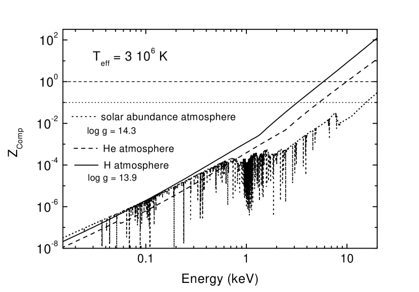
Figure 1: Comptonization parameter $Z_{\rm Comp}$ vs. photon energy for neutron star model atmospheres with different chemical compositions.

This qualitative analysis shows that Compton scattering can be significant for light element model atmospheres of isolated NS and we investigated this quantitatively in more detail.

3 Method of calculations

We computed model atmospheres of hot, isolated NSs subject to the constraints of hydrostatic and radiative equilibrium assuming planar geometry using standard methods (e.g.  Mihalas, 1978).

The model atmosphere structure for an NS with effective temperature $T_{\rm eff}$, surface gravity $g$, and given chemical composition is described by a set of differential equations. The first is the hydrostatic equilibrium equation

$$\frac{dP_{\rm g}}{dm}=g-4\pi\int_{0}^{\infty}H_{\nu}\,\frac{k_{\nu}+\sigma_{\nu}}{c}\,d\nu,$$ (3)

where

$$g=\frac{GM_{\rm NS}}{R^{2}_{\rm NS}\sqrt{1-R_{\rm S}/R_{\rm NS}}},$$ (4)

and when $R_{\rm S}=2GM_{\rm NS}/c^{2}$ is the Schwarzschild radius of the NS, $k_{\nu}$ opacity per unit mass due to free-free, bound-free, and bound-bound transitions, $\sigma_{\rm e}$ the electron (Thomson) opacity, $H_{\nu}$ Eddington flux, $P_{\rm g}$ a gas pressure, and the column density $m$ is determined as

$$dm=-\rho\,dz\,.$$ (5)

The variable $\rho$ denotes the gas density and $z$ is the vertical distance.

The second is the radiation transfer equation with Compton scattering taken into account using the Kompaneets operator (Kompaneets, 1957; Zavlin & Shibanov, 1991; Grebenev & Sunyaev, 2002):

$$\frac{\partial^{2}f_{\nu}J_{\nu}}{\partial\tau_{\nu}^{2}}=\frac{k_{\nu}}{k_{\nu}+\sigma_{\rm e}}\left(J_{\nu}-B_{\nu}\right)-\frac{\sigma_{\rm e}}{k_{\nu}+\sigma_{\rm e}}\frac{kT}{m_{\rm e}c^{2}}\times$$ (6)

$$x\frac{\partial}{\partial x}\left(x\frac{\partial J_{\nu}}{\partial x}-3J_{\nu}+\frac{T_{\rm eff}}{T}xJ_{\nu}\left(1+\frac{CJ_{\nu}}{x^{3}}\right)\right),$$

where $x=h\nu/kT_{\rm eff}$ is the dimensionless frequency, $f_{\nu}(\tau_{\nu})$ the variable Eddington factor, $J_{\nu}$ the mean intensity of radiation, $B_{\nu}$ the black body (Planck) intensity, $T$ the local electron temperature, and $C=c^{2}h^{2}\leavevmode\nobreak\ /\leavevmode\nobreak\ 2(kT_{\rm eff})^{3}$. The optical depth $\tau_{\nu}$ is defined as

$$d\tau_{\nu}=(k_{\nu}+\sigma_{\rm e})\,dm.$$ (7)

These equations have to be completed both by the energy balance equation

$$\int_{0}^{\infty}k_{\nu}\left(J_{\nu}-B_{\nu}\right)d\nu-\sigma_{\rm e}\frac{kT}{m_{\rm e}c^{2}}\times$$ (8)

$$\left(4\int_{0}^{\infty}J_{\nu}\,d\nu-\frac{T_{\rm eff}}{T}\int_{0}^{\infty}xJ_{\nu}(1+\frac{CJ_{\nu}}{x^{3}})\,d\nu\right)=0,$$

the ideal gas law

$$P_{\rm g}=N_{\rm tot}kT,$$ (9)

where $N_{\rm tot}$ is the number density of all particles, and also by the particle and charge conservation equations. We assume local thermodynamical equilibrium (LTE) in our calculations, so the number densities of all ionization and excitation states of all elements were calculated using Boltzmann and Saha equations. We take the pressure ionization effects into account on atomic populations using the occupation probability formalism (Hummer & Mihalas, 1988) as described by Hubeny et al. (1994).

For solving the above equations and computing the model atmosphere, we used a version of the computer code ATLAS (Kurucz, 1970, 1993), modified to deal with high temperatures. In particular, we take free-free and bound-free transitions into consideration for all ions of the 15 most abundant chemical elements, and about 25 000 spectral lines of these ions are also included; see Ibragimov et al. (2003) and Swartz et al. (2002) for further details. This code was also modified to account for Compton scattering (Suleimanov & Poutanen 2006; Suleimanov et al. 2006).

The scheme of calculations is as follows. First of all, the input parameters of the model atmosphere are defined: the effective temperature $T_{\rm eff}$, surface gravity $g$, and the chemical composition. Then a starting model using a grey temperature distribution is calculated. The calculations are performed with a set of 98 depth points $m_{\rm i}$ distributed logarithmically in equal steps from $m\approx 10^{-7}$ g cm^-2 to $m_{\rm max}$. The appropriate value of $m_{\rm max}$ is found from the condition $\sqrt{\tau_{\nu,\rm b-f,f-f}(m_{\rm max})\tau_{\nu}(m_{\rm max})}>$ 1 at all frequencies. Here $\tau_{\nu,\rm b-f,f-f}$ is the optical depth computed with only the true opacity (bound-free and free-free transitions, without scattering) taken into consideration. Satisfying this equation is necessary for the inner boundary condition of the radiation transfer.

For the starting model, all number densities and opacities at all depth points and all frequencies are calculated. We use 300 logarithmically equidistant frequency points in our computations. The radiation transfer equation (6) is non-linear and is solved iteratively by the Feautrier method (Mihalas, 1978, ; see also Zavlin & Shibanov 1991; Pavlov et al. 1991; Grebenev & Sunyaev 2002). We use the last term of Eq. (6) in the form $xJ_{\nu}^{i}(1+CJ_{\nu}^{i-1}/x^{3})$, where $J_{\nu}^{i-1}$ is the mean intensity from the previous iteration. During the first iteration we take $J_{\nu}^{i-1}=0$. Between iterations we calculate the variable Eddington factors $f_{\nu}$ and $h_{\nu}$, using the formal solution of the radiation transfer equation in three angles at each frequency. In the considered models 4-5 iterations are sufficient for achieving convergence.

We used the usual condition at the outer boundary

$$\frac{\partial J_{\nu}}{\partial\tau_{\nu}}=h_{\nu}J_{\nu},$$ (10)

where $h_{\nu}$ is the surface variable Eddington factor. The inner boundary condition is

$$\frac{\partial J_{\nu}}{\partial\tau_{\nu}}=\frac{\partial B_{\nu}}{\partial\tau_{\nu}}.$$ (11)

The outer boundary condition is found from the lack of incoming radiation at the NS surface, and the inner boundary condition is obtained from the diffusion approximation $J_{\nu}\approx B_{\nu}$ and $H_{\nu}\approx 1/3\times\partial B_{\nu}/\partial\tau_{\nu}$.

The boundary conditions along the frequency axis are

$$J_{\nu}=B_{\nu}$$ (12)

at the lower frequency boundary ($\nu_{\rm min}=10^{14}$ Hz, $h\nu_{min}$ $\ll kT_{\rm eff}$), and

$$x\frac{\partial J_{\nu}}{\partial x}-3J_{\nu}+\frac{T_{\rm eff}}{T}xJ_{\nu}\left(1+\frac{CJ_{\nu}}{x^{3}}\right)=0$$ (13)

at the upper frequency boundary ($\nu_{\rm max}\approx 10^{19}$ Hz, $h\nu_{\rm max}\gg kT_{\rm eff}$). Condition (12) means that at the lowest energies the true opacity dominates over scattering $k_{\nu}\gg\sigma_{\rm e}$, and therefore $J_{\nu}\approx B_{\nu}$. Condition (13) means that there is no photon flux along the frequency axis at the highest energy.

The solution of the radiative transfer equation (6) was checked for the energy balance equation (8), together with the surface flux condition

$$4\pi\int_{0}^{\infty}H_{\nu}(m=0)d\nu=\sigma T_{\rm eff}^{4}=4\pi H_{0}.$$ (14)

The relative flux error

$$\varepsilon_{H}(m)=1-\frac{H_{0}}{\int_{0}^{\infty}H_{\nu}(m)d\nu},$$ (15)

and the energy balance error as functions of depth

$$\varepsilon_{\Lambda}(m)=\int_{0}^{\infty}k_{\nu}\left(J_{\nu}-B_{\nu}\right)d\nu-\sigma_{\rm e}\frac{kT}{m_{\rm e}c^{2}}\times$$ (16)

$$\leavevmode\nobreak\ \leavevmode\nobreak\ \leavevmode\nobreak\ \leavevmode\nobreak\ \leavevmode\nobreak\ \leavevmode\nobreak\ \leavevmode\nobreak\ \leavevmode\nobreak\ \leavevmode\nobreak\ \leavevmode\nobreak\ \leavevmode\nobreak\ \leavevmode\nobreak\ \leavevmode\nobreak\ \leavevmode\nobreak\ \left(4\int_{0}^{\infty}J_{\nu}\,d\nu-\frac{T_{\rm eff}}{T}\int_{0}^{\infty}xJ_{\nu}(1+\frac{CJ_{\nu}}{x^{3}})\,d\nu\right)$$

were calculated, where $H_{\nu}(m)$ is radiation flux at any given depth $m$. This quantity is found from the first moment of the radiation transfer equation:

$$\frac{\partial f_{\nu}J_{\nu}}{\partial\tau_{\nu}}=H_{\nu}.$$ (17)

Temperature corrections were then evaluated using three different procedures. The first is the integral $\Lambda$-iteration method, modified for Compton scattering, based on the energy balance equation (8). In this method the temperature correction for a particular depth is found from

$$\Delta T_{\Lambda}=\frac{-\varepsilon_{\Lambda}(m)}{\int_{0}^{\infty}\left[(\Lambda_{\nu\leavevmode\nobreak\ diag}-1)/(1-\alpha_{\nu}\Lambda_{\nu\leavevmode\nobreak\ diag})\right]k_{\nu}(dB_{\nu}/dT)\,d\nu}.$$ (18)

Here $\alpha_{\nu}=\sigma_{\rm e}/(k_{\nu}+\sigma_{\rm e})$, and $\Lambda_{\nu\leavevmode\nobreak\ diag}$ is the diagonal matrix element of the $\Lambda$ operator (see details in Kurucz 1970). This procedure is used in the upper atmospheric layers. The second procedure is the Avrett-Krook flux correction, which uses the relative flux error $\varepsilon_{H}(m)$ and is performed in the deep layers. And the third one is the surface correction, which is based on the emergent flux error. See Kurucz (1970) for a detailed description of the methods.

The iteration procedure is repeated until the relative flux error is smaller than 1%, and the relative flux derivative error is smaller than 0.01%. As a result of these calculations, we obtain a self-consistent isolated NS model atmosphere, together with the emergent spectrum of radiation.

Our method of calculation was tested on a model for X-ray bursting NS atmospheres (Pavlov et al., 1991; Madej et al., 2004). We found that our models are in good agreement with these calculations.

4 Results

We use this method to calculate a set of hydrogen and helium isolated NS model atmospheres with effective temperatures 1, 2, 3, 5 $\cdot 10^{6}$ K and surface gravities $\log\leavevmode\nobreak\ g$ = 13.9 and 14.3 was calculated. Models with Compton scattering and Thomson scattering were computed for comparison. Part of the results are presented in Figs. 2 - 4.

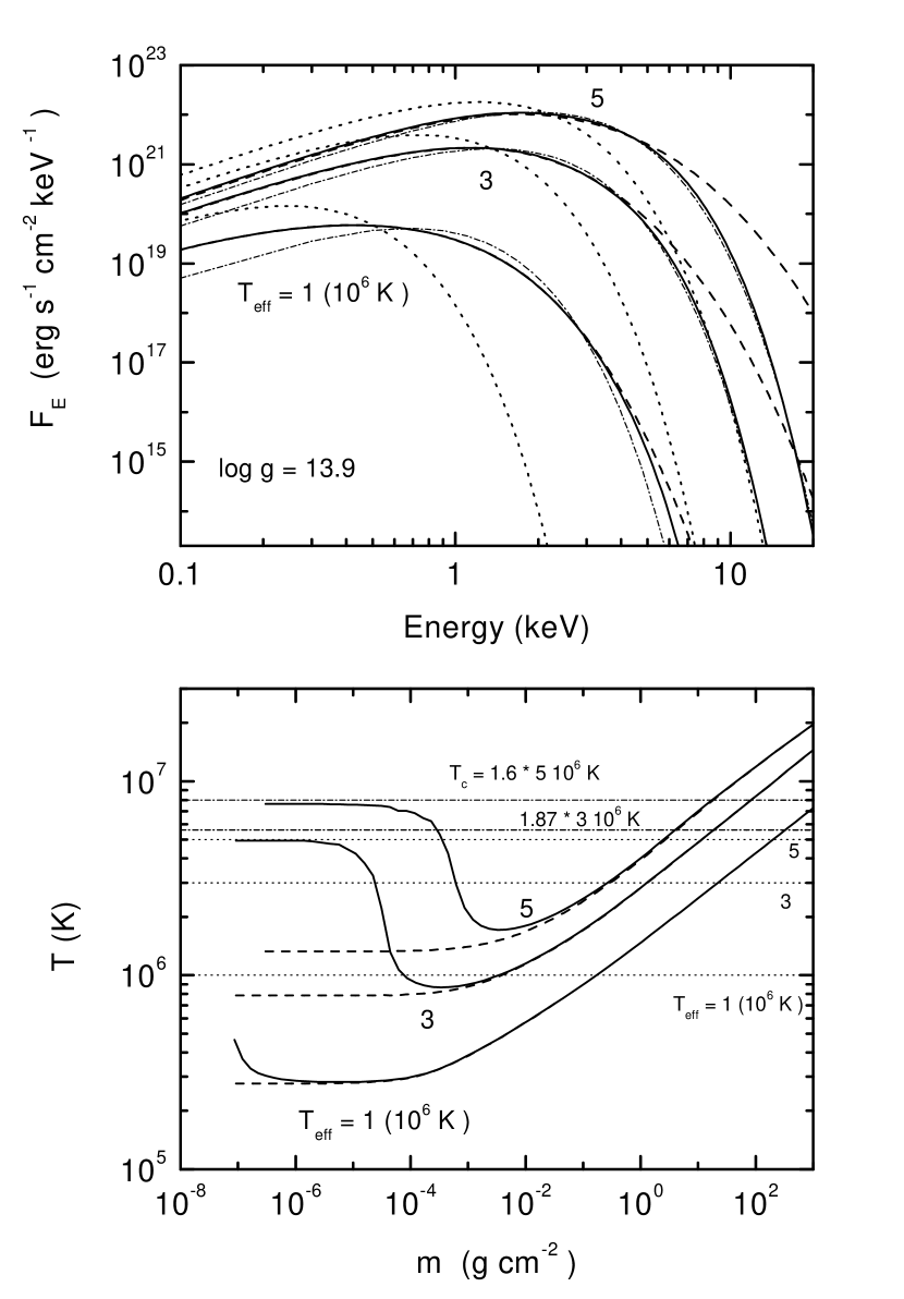
Figure 2: Top panel: Emergent (unredshifted) spectra of pure hydrogen, low gravity ($\log g$=13.9) NS model atmospheres. Solid curves - with Compton effect; dashed curves - without Compton effect; dotted curves - blackbody spectra; thin dash-dotted curves - diluted blackbody spectra with hardness factors 2.79, 1.87, and 1.6 for models with $T_{\rm eff}$ = 1,3 and 5$\cdot 10^{6}$ K. Bottom panel: Temperature structures of the corresponding model atmospheres. Effective and color temperatures are shown by dotted and dash-dotted lines, respectively.

The Compton effect is significant for the spectra of hot ($T_{\rm eff}\geq 3\cdot 10^{6}$ K) hydrogen model atmospheres at high energies (Fig. 2). The hard emergent photons lose energy and heat the upper layers of the atmospheres due to interactions with electrons. As a result, the high-energy tails of the emergent spectra become similar to Wien spectra. The temperature also increases in the upper layers of the model atmospheres and chromosphere-like structures appear. Temperatures of these structures are close to the color temperatures of the Wien tails of the emergent spectra. Moreover, the overall emergent model spectra of high temperature atmospheres in a first approximation can be presented as diluted blackbody spectra with color temperatures that are close to Wien tail color temperatures

$$F_{\rm E}=\frac{\pi}{f_{\rm c}^{4}}B_{\rm E}(T_{\rm c}),\leavevmode\nobreak\ \leavevmode\nobreak\ \leavevmode\nobreak\ \leavevmode\nobreak\ \leavevmode\nobreak\ \leavevmode\nobreak\ T_{\rm c}=f_{\rm c}T_{\rm eff},$$ (19)

where $f_{\rm c}$ is hardness factor and $F_{\rm E}$ is connected to $H_{\nu}$ as follows:

$$F_{\rm E}=4\pi H_{\nu}\leavevmode\nobreak\ \frac{d\nu}{dE},\leavevmode\nobreak\ \leavevmode\nobreak\ \leavevmode\nobreak\ \leavevmode\nobreak\ \leavevmode\nobreak\ \frac{d\nu}{dE}=\frac{1.6022\cdot 10^{-9}{\rm erg}/{\rm keV}}{h}.$$

These results are similar to those obtained for model atmospheres and emergent spectra of X-ray bursting NS in LMXBs (London et al., 1986; Lapidus et al., 1986; Ebisuzaki, 1987; Madej, 1991; Pavlov et al., 1991; Madej et al., 2004).

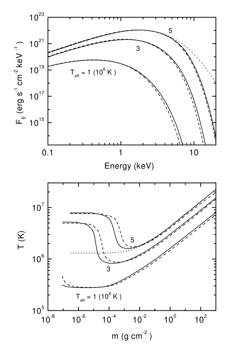
Figure 3: Top panel: Emergent (unredshifted) spectra of pure hydrogen NS model atmospheres with different surface gravities (solid curves - high gravity ($\log g$ = 14.3) models; dashed curves - low gravity models ($\log g$ = 13.9)). For comparison the model spectra without Compton effect are shown for the hottest high gravity model (dotted curve). Bottom panel: Temperature structures of the corresponding model atmospheres.

Table 1: The hardness factors $f_{c}$ for hydrogen and helium NS model atmospheres with different $\log g$ computed for models with Compton (C) and Thomson (T) scattering. The values in the brackets show the deviations $\varepsilon$ of the model spectra from diluted blackbody spectra with color temperature $T_{\rm c}=f_{c}T_{\rm eff}$ (see Eq. 20).

	Hydrogen models				Helium models
$T_{\rm eff}$	$\log\leavevmode\nobreak\ g$ = 13.9		$\log\leavevmode\nobreak\ g$ = 14.3		$\log\leavevmode\nobreak\ g$ = 13.9		$\log\leavevmode\nobreak\ g$ = 14.3
	C	T	C	T	C	T	C	T
$1\cdot 10^{6}$ K	2.79	2.69	2.86	2.81	2.83	2.81	2.83	2.82
	(0.30)	(0.32)	(0.32)	(0.33)	(0.35)	(0.35)	(0.37)	(0.36)
$2\cdot 10^{6}$ K	2.20	2.16	2.37	2.28	…	…	…	…
	(0.10)	(0.20)	(0.14)	(0.20)
$3\cdot 10^{6}$ K	1.87	1.91	1.97	1.99	2.05	2.04	2.15	2.12
	(0.05)	(0.15)	(0.07)	(0.14)	(0.09)	(0.13)	(0.11)	(0.14)
$5\cdot 10^{6}$ K	1.60	1.64	1.64	1.67	1.67	1.69	1.72	1.73
	(0.03)	(0.08)	(0.03)	(0.07)	(0.04)	(0.06)	(0.04)	(0.06)

The Compton scattering effect on the emergent model spectra of high gravity atmospheres is less significant (Fig. 3). The reason is a relatively small contribution of electron scattering to the total opacity in high gravity atmospheres compared to low gravity ones. The mass density in the high gravity models is higher, and the opacity coefficient (in cm²/g) is independent of the density for electron scattering and proportional to the density for free-free transitions. In the presented models, H and He are practically fully ionized. Therefore, free-free transitions dominate the true opacity.

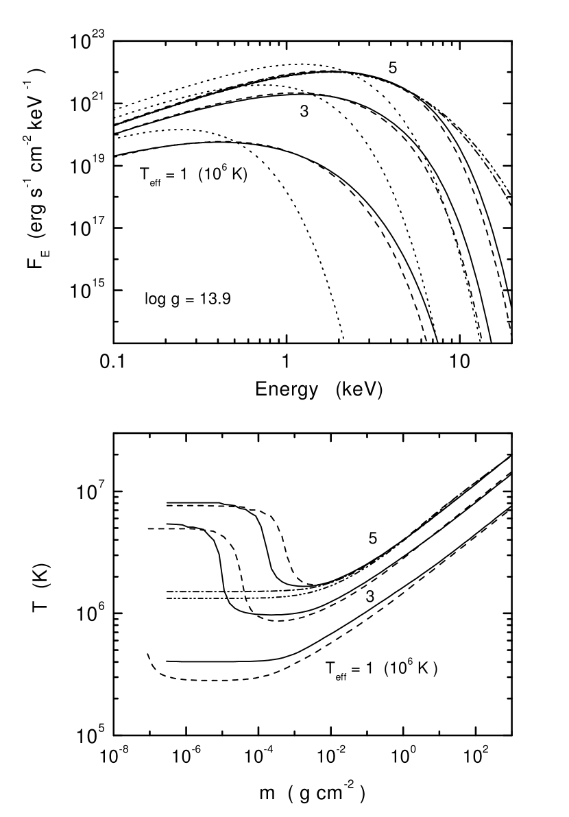
Figure 4: Top panel: Emergent (unredshifted) model spectra of pure helium, low gravity ($\log g$ = 13.9) NS model atmospheres. For comparison the model spectra of pure hydrogen atmospheres are shown by dashed curves. Model spectra of the hottest atmospheres without Compton effect are shown by dash-dotted and dash-dot-dotted curves. Bottom panel: Temperature structures of the corresponding model atmospheres.

The Compton scattering effect on helium model atmospheres is also less significant than on hydrogen model atmospheres with the same $T_{\rm eff}$ and $\log\leavevmode\nobreak\ g$ (Fig. 4). The reason is the same as in the case of high gravity models. The ratio of electron scattering to a true opacity is smaller in the helium models. It is interesting to notice that, in the case of Thomson scattering, the emergent model spectra of helium atmospheres are softer than those of the hydrogen atmospheres. But in models where Compton scattering is taken into consideration, the spectra of helium atmospheres are harder than the spectra of hydrogen models.

We fitted the calculated emergent spectra of this set of models by the diluted blackbody spectra in energy range 0.2 - 10 keV. We computed the value

$$\varepsilon=\frac{1}{N}\leavevmode\nobreak\ \Sigma_{j=1}^{N}\leavevmode\nobreak\ \left(1-\frac{B_{\rm E,\,j}(f_{c}T_{\rm eff})}{F_{\rm E,\,j}}\right)^{2}$$ (20)

as a measure for the deviation of the model spectrum $F_{\rm E}$ from the diluted blackbody spectrum $B_{\rm E}$. Here $N$ is the number of energy points E, j between 0.2 and 10 keV. Corresponding hardness factors are presented in the Table 1 together with $\varepsilon$. Spectra of the hot models with Compton scattering are better approximated by a diluted black body, especially for hydrogen models. But the hardness factors are changing only slightly. Data from Table 1 can be used for interpretating of observed isolated NS X-ray spectra. The hardness factor can be found from these data if the observed color temperature $T_{c}^{\infty}$ and gravitational redshift $z$ of the NS are known. As soon as $f_{\rm c}$ is determined, the apparent NS radius $R_{\infty}$ can be found from the observed flux $f_{\rm E}$ with the relation:

$$f_{\rm E}=\frac{\pi}{f_{\rm c}^{4}}B_{\rm E}(T_{\rm c}^{\infty})\frac{R_{\infty}^{2}}{d^{2}},$$ (21)

where $d$ is distance to the NS.

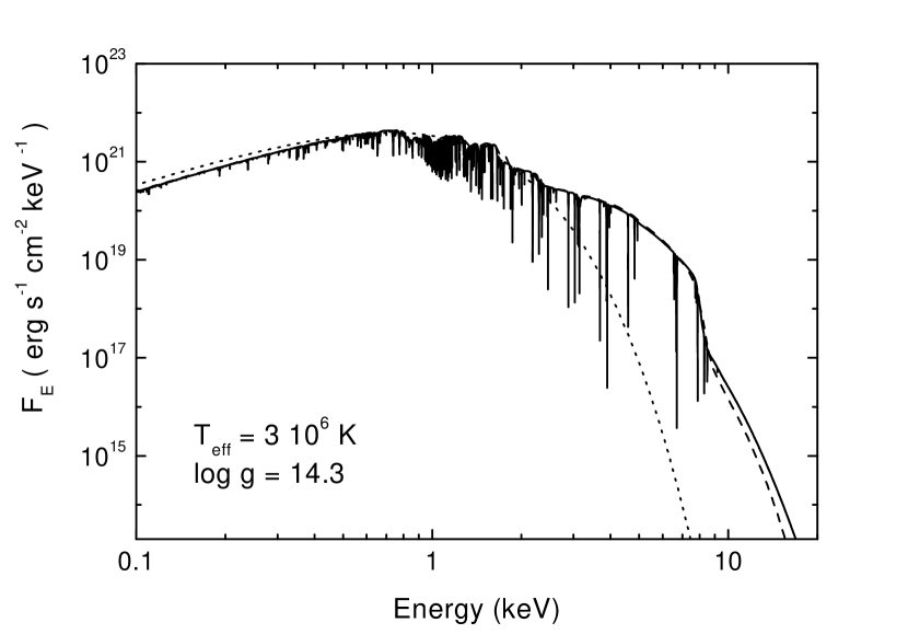
Figure 5: Emergent (unredshifted) model spectra of high gravity ($\log g$ = 14.3) NS atmospheres with the solar abundance of 15 most abundant heavy elements with (dashed curve) and without (solid curve) Compton scattering. The dotted curve is the corresponding blackbody spectrum.

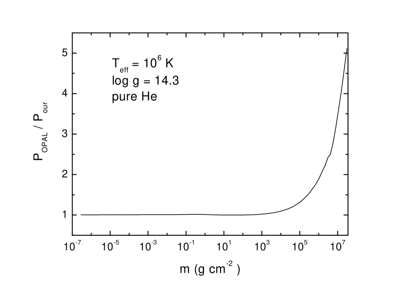
Figure 6: Ratio of the gas pressure obtained by interpolation from OPAL EOS tables (see text) to the gas pressure from our calculations for the pure He model with $T_{\rm eff}$ = 10⁶ K and $\log g$ = 14.3.

We also computed one isolated NS model atmosphere with solar chemical abundance and $T_{\rm eff}=3\cdot 10^{6}$ K and $\log\leavevmode\nobreak\ g$=14.3 (see Fig. 5). The model was calculated with Thomson and Compton scattering and we found that the Compton effect on the emergent spectrum is very small.

In our calculations we ignored deviations from the ideal gas EOS (9) other than the ionization by pressure. We checked this approximation as follows. We found gas pressures from the temperatures and densities at all depth points for a pure helium atmosphere with $T_{\rm eff}$ = 10⁶ K and $\log g$ = 14.3 by interpolation from the OPAL EOS tables. We compared the obtained gas pressures with the values calculated in our model. The ratio of these two gas pressures are shown in Fig. 6. We find that the OPAL EOS gas pressure is equal to the gas pressure in our model with an accuracy of about 1 % up to column density $\sim$ 10³ g cm^-2. At larger depths the OPAL EOS gas pressure is significantly larger due to partial electron degeneracy. All of the emergent photons are emitted at column densities lower than 10³ g cm^-2 (for example, photons with energy 10 keV are emitted at column density $\sim$ 20 g cm^-2). The distinction between the OPAL EOS and (9) must be smaller for models with larger $T_{\rm eff}$ and for pure hydrogen models. Therefore, the EOS deviation from (9) at the deepest atmospheric layers cannot change the emergent model spectra that we calculated here.

5 Conclusions

We have presented the results of calculations for the hot model atmospheres of isolated NSs with low magnetic fields and different chemical compositions. The Compton effect is taken into account. We investigated the importance of Compton scattering for the emergent spectra of these models. The main conclusions follow.

Emergent model spectra of hydrogen and helium NS atmospheres with $T_{\rm eff}\geq 1\cdot 10^{6}$ K are changed by the Compton effect at high energies ($E>5$ keV), and spectra of the hottest ($T_{\rm eff}\geq 3\cdot 10^{6}$ K) model atmospheres can be described by diluted blackbody spectra with hardness factors $\sim$ 1.6 - 1.9. At the same time, however, the spectral energy distribution (SED) of these models are not significantly changed at the maximum of the SED (at energies 1-3 keV), and effects on the color temperatures are not strong.

The Compton effect is the most significant for hydrogen model atmospheres and in low gravity models. Emergent model spectra of NS atmospheres with solar metal abundances are affected by Compton effects only very slightly.