Integral Field Spectroscopy of the Quadruply Lensed Quasar 1RXS J1131-1231: New Light on Lens Substructures

Abstract

We have observed the quadruply lensed quasar 1RXS J1131-1231 with the integral field spectrograph mode of the Kyoto Tridimensional Spectrograph II mounted on the Subaru telescope. Its field of view has covered simultaneously the three brighter lensed images A, B, and C, which are known to exhibit anomalous flux ratios in their continuum emission. We have found that the [OIII] line flux ratios among these lensed images are consistent with those predicted by smooth-lens models. The absence of both microlensing and millilensing effects on this [OIII] narrow line region sets important limits on the mass of any substructures along the line of sight, which is expressed as $M_{\rm E}<10^{5}M_{\odot}$ for the mass inside an Einstein radius. In contrast, the H$\beta$ line emission, which originates from the broad line region, shows an anomaly in the flux ratio between images B and C, i.e., a factor two smaller C$/$B ratio than predicted by smooth-lens models. The ratio of A$/$B in the H$\beta$ line is well reproduced. We show that the anomalous C$/$B ratio for the H$\beta$ line is caused most likely by micro/milli-lensing of image C. This is because other effects, such as the differential dust extinction and/or arrival time difference between images B and C, or the simultaneous lensing of another pair of images A and B, are all unlikely. In addition, we have found that the broad H$\beta$ line of image A shows a slight asymmetry in its profile compared with those in the other images, which suggests the presence of a small microlensing effect on this line emitting region of image A.

1 INTRODUCTION

Gravitational lensing is an important probe for the mass distribution of lensing galaxies as well as for the internal structure of lensed sources (e.g., Kochanek et al., 2006). Quadruply lensed quasars are particularly useful in this regard since the positions and flux ratios of the lensed images provide strong constraints on lens models, and provide far more observational information than doubly imaged systems. For instance, recently revealed quads with “anomalous flux ratios”, namely flux ratios which are unexplained in smooth-lens models, suggest the presence of numerous substructures in the lensing galaxy (e.g., Mao & Schneider, 1998; Metcalf & Madau, 2001; Chiba, 2002; Dalal & Kochanek, 2002; Schechter & Wambsganss, 2002; Keeton, 2003). Whether or not these substructures correspond to cold dark matter (CDM) subhalos (milli-lensing), stellar populations (micro-lensing), or differential reddening by dust, remains an issue, and depends on the lens system (e.g., Chiba et al., 2005). It is of particular interest to assess whether there is a high level of substructures or subhalos in galaxy-sized halos, as predicted in CDM models (Klypin et al., 1999; Moore et al., 1999).

A technique to distinguish the origin of anomalous flux ratios was proposed by Moustakas & Metcalf (2003), utilizing spectroscopic information of lensed quasars. If we take into account a finite (i.e., not point-like) source size of a quasar heart, which consists of a small continuum emitting region (CR) with typical size $R_{\rm S}$ of $\sim 10^{-4}$ pc, broad line region (BLR) with $R_{\rm S}\sim 1$ pc, and narrow line region (NLR) with $R_{\rm S}\gtrsim 100$ pc, then the lensing magnification will be functions of these source sizes and the mass of any substructure inside its Einstein angle, $M_{\rm E}$ (i.e., either CDM subhalos with a mass $M_{\rm E}\sim 10^{7-9}M_{\odot}$ or stars with $M_{\rm E}\sim 1M_{\odot}$). If CDM subhalos are responsible for anomalous flux ratios, then they can magnify both the CR and BLR because their Einstein radii (projected onto the distance of the quasar), $r_{\rm E}\sim 0.01(M_{\rm E}/M_{\odot})^{1/2}h^{-1/2}$ pc (where $h=H_{0}/100$ km s^-1 Mpc^-1), are larger than the sizes of the CR and BLR. The NLR may be magnified as well, depending on the upper mass of the CDM subhalos. On the other hand, stars would be unable to magnify emission lines from either the BLR or NLR, while still magnifying the CR. As a consequence, depending on the nature of substructure, the fluxes of emission lines in each of the lensed images that show anomalous (continuum) flux ratios can be either magnified or unchanged.

The observations of multiply lensed objects with an integral field spectrograph (IFS) is useful in this study, since it provides simultaneous information among quasar images both spatially and spectrally (e.g., Metcalf et al., 2004; Wayth et al., 2005). The IFS is more superior to conventional slit spectroscopic techniques in the following aspects: (1) Slit spectroscopic observations would require separate observations for each pair of components. This not only requires more observing time but also introduces significant errors and uncertainties for relative flux measurements since exposures for each pair are carried out in different observational conditions. (2) IFS allows us to optimize the relative flux measurements after the observations, in terms of determining the size and center positions of the apertures used for photometry.

In this paper, we report on our spectroscopic mapping of the quadruply imaged quasar, 1RXS J1131$-$1231, which shows anomalous flux ratios, using the IFS mode of Kyoto tridimensional spectrograph II (Kyoto 3DII: Sugai et al., 2000, 2002, 2004) mounted on the Subaru 8.2-m telescope. This lens system is nearly unique among known gravitationally lensed systems in that it brings together rare properties, including the quadruplicity, a bright optical Einstein ring, a small redshift, and high amplification (Sluse et al., 2003, hereafter S03). S03 measured redshifts of 0.658 and 0.295 respectively for the quasar and the lensing galaxy. The lens shows three roughly co-linear highly magnified images, A, B, and, C. This configuration emerges if the quasar is close to and inside a cusp point of the astroid caustic for an elliptical lens (see also Figure 7 shown in §4). In such a lens system associated with a cusp singularity, there exists a universal relation between the image fluxes, $(F_{B}+F_{C})/F_{A}=1$ (e.g., Mao & Schneider, 1998), whereas the observed flux ratios violate these rules significantly [$(F_{B}+F_{C})/F_{A}\simeq 2.1$ in the $V$ band and $2.2$ in the $R$ band (S03)]. The flux ratios appear to be changing with time, as a result of microlensing effects on some of the images. Time delay effects between the images do not play a role in the flux ratio anomaly because simple smooth-lens models predict only a day or a fraction of a day for the time delays between images A, B, and C (Sluse et al., 2006; Claeskens et al., 2006). Several different lens models with smooth mass distribution have been constructed to attempt to reproduce the image positions, flux ratios, and time delays of this lens system. But it appears that one requires a high-order lens structure in addition to a simple ellipsoidal lens, in the form of an octupole component or an unidentified satellite (Claeskens et al., 2006; Morgan et al., 2006, hereafter M06).

Armed with the IFS mode of Kyoto 3DII, we measured the emission-line fluxes of both the BLR H$\beta$ and the NLR [OIII]$\lambda\lambda$4959,5007 for images A, B, and C simultaneously. The measurements of the line fluxes are more reliable than those of the continuum because there are no contributions from the lensing galaxy, the redshift of which differs from the quasar’s. The H$\beta$ and [OIII] lines are very close in wavelength, so that the effect of differential reddening between them is almost totally negligible. The unique fine sampling of $\sim 0^{\prime\prime}.1$, together with the simple shape of the point spread function and Subaru’s excellent image quality, provides the most suitable method for measuring the relative line fluxes.

This paper is organized as follows. §2 describes the observations and method for data reduction. Spectra of images A, B, and C and flux ratios between each image pair are shown in §3. §4 is devoted to discussion and conclusions.

2 OBSERVATIONS AND REDUCTION

We observed 1RXS J1131-1231 on 2005 February 8 with the IFS mode of the visitor instrument Kyoto 3DII, mounted on the Subaru. We used the atmospheric dispersion corrector installed at the Subaru Cassegrain focus (Iye et al., 2004). This enabled us to obtain the atmospheric-dispersion-free data cube without having to apply a correction during the data reduction (e.g., Sugai et al., 2005). The IFS mode uses an array of $37\times 37$ lenslets, enabling us to obtain spectra of $\sim 10^{3}$ spatial elements. The spectral range from $7300\AA$ to $9150\AA$ was observed in each of two one-hour exposures. With the spatial sampling of $0^{\prime\prime}.096$ lenslet^-1 (Sugai et al., 2004), the field of view of $\sim 3^{\prime\prime}$ covered the three brighter quasar images. The target was located at the same position of the lenslet array during the two exposures. Since the positional difference derived from the reconstructed data cubes was small, within a few tenths of a lenslet (i.e., a few $\times 0^{\prime\prime}.01$), we combined them without any offset between them. The spatial resolution was stable during the observations, and was determined to be $0^{\prime\prime}.5$-$0^{\prime\prime}.6$ from a strong “point”-like H$\beta$ emission-line distribution in the quasar image A (see § 3).

We used halogen lamp spectral frames for the flat fielding. These frames were obtained immediately before and after each of the target frames, with the same optical setting as the target frames. Since our calibration optics exactly simulates the telescope optics, i.e, since it provides the same micropupil images as the telescope does, it properly corrects differences in the lenslet-to-lenslet response (and efficiency). The uniformity of a flat-fielded reconstructed image is $1.5\%$ (1 $\sigma$). The wavelength calibration was carried out using He and Ne lamps, whose spectra were also taken immediately before and after each of the target frames. We measured that the calibration lamp line positions changed only by 0.1 pixel ($\sim 0.3\AA$) along the spectral direction during the whole sequence of observations. This corresponds to a systematic uncertainty in the wavelength calibration. Moreover, the technique of micropupil spectroscopy (Sugai et al., 2006) provides us with an accuracy in the relative wavelength calibration of $\sim 0.2\AA$, which has been determined within each of the calibration lamp frames. The full width at half maximum of the instrumental line profile was measured as $7\AA$, which corresponds to 260 km s^-1. In order to improve signal-to-noise ratios in target spectra, we smoothed them in wavelength by convolution with a gaussian profile so that the resultant velocity resolution was 390 km s^-1. The sky subtraction was carried out using simultaneous sky spectra. This is particularly important for longer wavelengths, where the sky emission lines are strong. For an accurate sky subtraction the Kyoto 3DII has two separate fields of view: one for the target and the other smaller one for sky, which is located $33^{\prime\prime}$ away from the target (Sugai et al., 2006). The averaged sky spectrum was subtracted from each target lenslet spectrum (see § 3).

The IFS data of the spectroscopic standard star HD93521 were used for the instrument response curve correction as well as for absolute flux density calibration. The extinction curve at Mauna Kea (CFHT Observatory Manual, http://www.cfht.hawaii.edu/Instruments/ ObservatoryManual/) was used to correct for the effects of airmass in both the target object and standard star spectra. The airmasses were 1.38 and 1.22 for the target frames and 1.23 for the standard star frames. The atmospheric conditions were checked using a guide star count log and were determined to have been non-photometric. We roughly estimate the uncertainty of absolute flux density calibration to be about $\pm 20\%$.

3 SPECTRA OF QUASAR IMAGES A, B, AND C

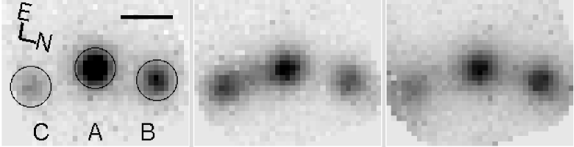
Figure 1: Images extracted from our IFS data. (left) Continuum-subtracted H$\beta$(+FeII$\lambda$4924) line image. The spectra have been integrated for the observed wavelength region from $7947\AA$ to $8162\AA$. The continuum level has been determined in wavelength regions from $7878\AA$ to $7947\AA$ and from $8399\AA$ to $8469\AA$. The length of a bar to the upper right is $1^{\prime\prime}$. The apertures used for obtaining spectra for quasar images, such as spectra in Figure 2, are shown with circles. North is at $102^{\circ}$ clockwise from the top. (middle) Continuum(+FeII$\lambda$5018)-subtracted [OIII]$\lambda$5007 line image. The spectra have been integrated for the observed wavelength region from $8247\AA$ to $8300\AA$. The “continuum” level has been determined in wavelength regions from $8221\AA$ to $8247\AA$ and from $8300\AA$ to $8343\AA$. (right) Line-free continuum image. The spectra have been integrated for the observed wavelength regions from $7878\AA$ to $7947\AA$ and from $8399\AA$ to $8469\AA$.

Figure 1 shows line images and a line-free continuum image that have been obtained from the IFS data. We find an extended component of the [OIII] emission connecting quasar images A and C. Such an extended component is not seen between quasar images A and B. The spatial distribution of the line-free continuum emission is similar to that of the H$\beta$ emission rather than the [OIII] emission. Despite the severe contamination from the host galaxy (§ 3.1), the continuum is much fainter in image C than in image B. Figure 2 (upper) shows the spectra of quasar images A, B, and C that have each been extracted with an 8-lenslet, i.e. a circular aperture with a diameter $0^{\prime\prime}.77$. An aperture of this size includes $\sim 60$ % of the total flux of a point source. The aperture centers have been determined from the H$\beta$ image shown in Figure 1. The relative positions of these centers are consistent, to within several milliarcseconds, with peak positions obtained by M06 using the Hubble Space Telescope. As an example, the lower panel in Figure 2 shows the spectrum of image A both with and without sky subtraction in order to demonstrate the effectiveness of the sky subtraction as described in § 2.

3.1 Comparison Between A and B

If all the emission from the quasar is magnified in the same manner within each quasar image, we should be able to completely subtract the spectrum of one quasar image with the spectrum of another quasar image by scaling the latter with an appropriate factor. If this is not the case, e.g. when the NLR line is magnified only by a macrolens while the BLR line is further magnified by a milli/micro-lens, it should be impossible to subtract these two lines completely with a single multiplicative factor. Using such spectral fittings, we derive the flux ratios in the BLR and in the NLR below. We do not attempt to derive the flux ratios in the continuum, which is severely contaminated by the quasar host galaxy.

Figure 3 (upper) shows a comparison between quasar images A & B. The spectrum of image A has been fit, using the least squares method, in the [OIII] and the line-free continuum emission wavelength regions according to the following equation: $f_{A}(\lambda)=b_{0}\times f_{B}(\lambda)-b_{1}\times(\lambda/8000\AA)^{b_{2}}$, where $f_{A}(\lambda)$ and $f_{B}(\lambda)$ are the flux densities of images A and B, respectively. The fitting parameter $b_{0}$ determines the scaling factor, while $b_{1}$ and $b_{2}$ are used to remove the smooth continuum. The spectrum has been fit with $b_{0}=1.63$. Similarly, we have fit the spectrum of image A in the broad H$\beta$ and the continuum wavelength regions (Figure 3 (lower)). The broad H$\beta$ in image A seems to have only slightly weaker emission in the bluer wing, compared with that in the scaled image B. The best fit $b_{0}$ is 1.74. We therefore conclude that the flux ratios A$/$B in the [OIII] and broad H$\beta$ emission lines are $1.63^{+0.04}_{-0.02}$ and $1.74^{+0.07}_{-0.12}$ respectively, where the uncertainties are derived as discussed in § 3.3. In order to compare these values with the ratio predicted by macrolens models, we have constructed a smooth-lens model with a singular isothermal ellipsoid plus an external shear (Kassiola & Kovner, 1993; Kormann et al., 1994), based on the quasar image positions obtained by M06. A slight offset of the halo center with respect to the lensing galaxy center has been allowed. This model predicts an A$/$B ratio of 1.66. The smooth-lens models constructed by S03 and by Blackburne et al. (2006, hereafter BPR06), with a singular isothermal sphere plus an external shear, also predicts a similar ratio of 1.75 - 1.70. We conclude therefore that the measured ratios are close to those predicted by smooth-lens models. The required offset for the spectral fitting, i.e. non-zero $b_{1}$, is likely caused primarily by contamination from the quasar host galaxy continuum. The contamination from the lensing galaxy is small since it is located outside of our field of view: $\sim 2^{\prime\prime}.1$ (e.g., M06, ) down from image A in Figure 1. Figure 1 (right) suggests that the contribution of the lensing galaxy is less than $6\times 10^{-18}$ erg cm^-2 s^-1 $\AA^{-1}$ and actually much smaller since we do not detect any signature of it even at positions that are closer to its center.

3.2 Comparison Between B and C

We have compared the spectra of images B and C using the same method as in § 3.1. When we scale the spectra according to the [OIII] line emission (Figure 4 (upper)), we find differences in the H$\beta$. The H$\beta$ profile also differs in these two spectra. Figure 4 (lower) shows the same comparison but with the C spectrum scaled according to the broad H$\beta$ emission. We find differences in the [OIII] lines and in the narrow line (NL) H$\beta$. The redshift of the NL H$\beta$ matches that of the [OIII] line ($z_{heliocentric}=0.6542\pm 0.0001(1\sigma)$, where the uncertainty includes the accuracy of [OIII] line peak determination as well as the wavelength calibration uncertainties). The “NL-subtracted” spectrum in Figure 4 (upper) suggests that the broad line (BL) H$\beta$ is more symmetric than the original BL$+$NL H$\beta$, and is redshifted with respect to the NL H$\beta$ ($z_{heliocentric}=0.6581\pm 0.0001$ for BL H$\beta$). We have measured an asymmetry parameter, $A$, of the H$\beta$ emission for both the original and residual spectrum of image B: $A=(HWHM_{Red}-HWHM_{Blue})/FWHM$, where $HWHM_{Red}$ and $HWHM_{Blue}$ represent the half-widths at half-maximum flux density of the red and blue wings of the profile respectively (Wills et al., 1993). Our measurements have shown that A=0.32 and A=0.08 respectively, for the original BL$+$NL H$\beta$ and the residual BL H$\beta$. The difference in the H$\beta$ profile between images B and C is caused by different fractions of NL contribution. The above comparisons lead us to conclude that the flux ratio between images B and C largely depends on where the lines originate: the BLR or the NLR. The flux ratio C$/$B in the [OIII] line is $1.19^{+0.03}_{-0.12}$, whereas it is $0.46^{+0.02}_{-0.03}$ in the BL H$\beta$ line. As before, uncertainties are derived as in § 3.3. Compared to predictions of the smooth-lens models, this is larger only by a factor of $\sim 1.2$ in [OIII] but is smaller by a factor of $\sim 2.1$ in the BL H$\beta$. Table 1 summarizes the flux ratios obtained between the quasar images A, B, and C, together with the ratios expected from the smooth-lens models.

In order to derive the H$\beta$ and [OIII] flux ratios between quasar images, we have used the simple scaling and fitting methods above, without using any template for the FeII line emission. This is because we have found that the observed FeII line ratios differ slightly from the well-established I Zw 1 template (Véron-Cetty et al., 2004) and that the FeII is better subtracted by the scaling between quasar images themselves.

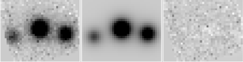
Figure 5: (left) Continuum-subtracted H$\beta$(+FeII$\lambda$4924) line image. The same as that in Figure 1. (middle) Model image with three point sources that have flux ratios shown in Table 1 and have the common Moffat function profile. (right) The residual image ((left)-(middle)). These images are shown in the same grayscale.

Figure 5 demonstrates in another way the suitability of our scaling method. The H$\beta$ residual image has been created by subtracting three point sources with the H$\beta$ flux ratios derived above, from the H$\beta$ image shown in Figure 1. The residuals have an rms of only $3\%$ of the peak value of quasar image A.

3.3 Uncertainty Estimates

The uncertainties of the measured flux ratios in Table 1 have been estimated as follows. First we have tried another spectrum fitting procedure that differs from the procedure used in Figures 3 and 4. In this new fitting procedure, we fit the line emission after removing the continuum emission from each image spectrum, rather than fitting the line and continuum emission simultaneously. This altered the flux ratios slightly, by 0.00–0.05. Secondly we have estimated the mutual flux contamination between images due to point-like components, by using the model of three point sources shown in Figure 5. In the $0^{\prime\prime}.77$ aperture the contamination in broad H$\beta$ for images A, B, and C are 1 %, 3 %, and 5 % respectively. The effects on the A$/$B and C$/$B ratios are $-2\ \%$ and $+2\ \%$. In the same aperture the mutual contaminations between the “point-like” [OIII] components (see § 4) are estimated as 2 %, 3 %, and 2 % respectively. The effects on the A$/$B and C$/$B ratios are $-1\%$. Thirdly we have derived the flux ratios with the simultaneous (line $+$ continuum) fitting procedure, but using successively smaller apertures, down to the size of a 4-lenslet ($0^{\prime\prime}.38$ diameter). While the C$/$B ratio in [OIII] decreases by up to 0.07 as the aperture size is reduced, the other ratios vary by no more than $\pm 0.02$. These differences should in practice include various effects: mutual contamination, contributions from the spatially extended components, readout and photon noise, and flat fielding uncertainties. Lastly we have considered the uncertainty of the A$/$B ratio in the broad H$\beta$ emission due to the slight difference in its wing profile between images A and B (§ 3.1). When, during the fitting, we reduce the weighting of each blue wing data point by half, the A$/$B ratio is 1.76. When we reduce the weighting of each red wing data point by half, on the other hand, the A$/$B ratio is 1.69. We have taken all the above into consideration when determining the uncertainties of the measured flux ratios in Table 1. The effects of uncertainties of the aperture center positions are negligible because the positional uncertainties are smaller than one tenth of a lenslet.

4 DISCUSSION AND CONCLUSIONS

Anomalous flux ratios in lensed images can be induced by substructure in a host lens. As a reference for investigating such substructure lensing, we estimate the angular size of the radius of a line-emitting region, $\theta_{\rm S}$, and of an Einstein radius for a lens substructure, $\theta_{\rm E}$, based on the set of cosmological parameters $\Omega=0.3$, $\Lambda=0.7$, and $h=0.7$. A source image with radius $R_{\rm S}$ at the redshift 0.658 of the quasar has an angular size of $\theta_{\rm S}\simeq 1.4\times 10^{-4}(R_{\rm S}/1{\rm pc})$ arcsec. For comparison, a lens having a mass $M_{\rm E}$ inside an Einstein angle yields $\theta_{\rm E}\simeq 6.7\times 10^{-7}(M_{\rm E}/0.1M_{\odot})^{1/2}$ arcsec for the lens redshift of 0.295. Thus, a dimensionless ratio $\xi\equiv\theta_{\rm S}/\theta_{\rm E}$ showing the degree of a lensing effect (BPR06) is given as $\xi\simeq 200(R_{\rm S}/1{\rm pc})(M_{\rm E}/0.1M_{\odot})^{-1/2}$. Wyithe et al. (2002) showed, based on detailed lensing simulations, that $\theta_{\rm E}$ must be at least an order of magnitude smaller than $\theta_{\rm S}$ for no magnification. This leads us to require that $\xi\gtrsim 10$ if there is no additional magnification of an image by a lens substructure. Otherwise an image should be subject to flux anomaly.

As presented in Table 1, the flux ratios for the [OIII] line emission, which originates from the NLR with $R_{\rm S}\gtrsim 100$ pc, are basically in agreement with those of a standard smooth lens consisting of an elliptical lens and an external shear. Also, the [OIII] flux ratios appear to be inconsistent with M06’s lens model, which posits a massive satellite with $\sim 5\times 10^{10}M_{\odot}$ near image A in order to reproduce their time delay measurements. Such a massive lens perturber would affect the [OIII] flux significantly. The basic agreement of the [OIII] flux ratios with the smooth-lens model predictions suggests not only the validity of the smooth-lens models but also the absence of millilensing effects. A star with subsolar mass is unable to magnify the NLR because $\xi\sim 2\times 10^{4}$ for $R_{\rm S}=100$ pc and $M_{\rm E}=0.1$ $M_{\odot}$. A more massive substructure such as a CDM subhalo, even if it exists near the light path to the NLR, is tightly constrained to have $M_{\rm E}<10^{5}$ $M_{\odot}$.

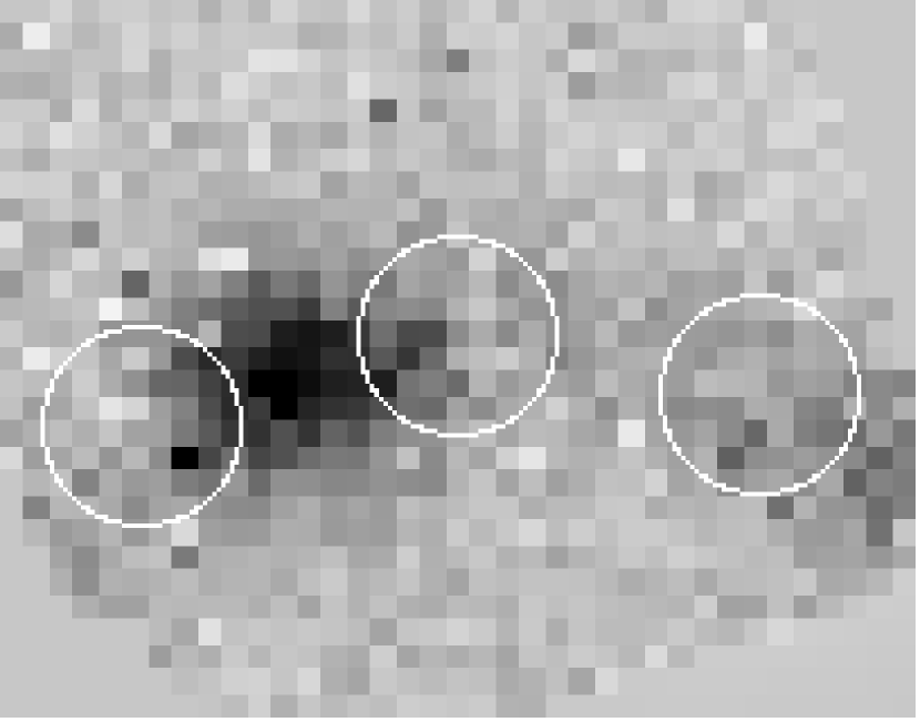
Figure 6: Three-point-source-model subtracted [OIII]$\lambda$5007 line image, where the three point sources have flux ratios shown in Table 1 and have the common Moffat function profile as determined from the broad H$\beta$ point source. The apertures shown with circles are the same as those in Figure 1.

It is worth noting that the observed flux ratio C$/$B in the [OIII] line emission slightly differs from the model predictions at about the 20 % level, while the flux ratio A$/$B is well reproduced. This slight inconsistency with a smooth-lens model might be caused by a substructure with an extended instead of point-like mass distribution being located at one of the lensed images. Inoue & Chiba (2005) showed that for a substructure with a singular isothermal density distribution, the flux ratio can be changed by about 20 % from a smooth-lens prediction even if $\xi\gtrsim 10$, provided the substructure is just centered at the source image. Alternatively, and perhaps more likely, is the effect of an asymmetric structure or light distribution intrinsic to the NLR (e.g., Schmitt et al., 2003). In contrast, a smooth-lens model assumes a uniform and circularly-symmetric NLR as a source image. In fact, this effect can partially be seen as an extension of the [OIII] emission between images A and C as well as a slight extension of image B in the direction opposite to images A and C (Figure 1). This indicates that we have spatially resolved the NLR itself. Figure 6 emphasizes these extensions in the subtraction of three “point” source models from the [OIII] line image. The total [OIII] flux of the extended emission between images A and C is about a half of that of the point-like component of image A at our resolution. The fractional contributions from the extended emission components are 16 % – 20 % even in the $0^{\prime\prime}.77$ apertures of the quasar images. This causes the slight aperture dependence of [OIII] flux ratios between images (particularly the C$/$B ratio) as described in § 3.3. We have found, based on the lens modeling, that asymmetric configurations of lensed images can be caused by asymmetric structure in the NLR in the north-south direction, i.e. if the north side of the NLR is more luminous or more spatially extended than the south side. An example of such models is shown in Figure 7. This asymmetry in the lensed images of the NLR would be attributed to a slight difference between the measured flux ratios inside a finite aperture and the smooth-lens predictions based on a uniform and circularly-symmetric source.

In contrast to the [OIII] line emission, the broad-line H$\beta$ emission, which originates from the BLR, shows a significant difference to the model for the flux ratio C$/$B , i.e. C$/$B$=0.46$ compared with the predicted ratio of $0.91\sim 1.00$, while the flux ratio A$/$B is well reproduced by a smooth lens. This anomaly for the flux ratio C$/$B in the H$\beta$ line emission is caused neither by effects of (i) dust extinction nor (ii) time delay on lensed images, as argued below. (i) There are no effects of dust extinction on the H$\beta$ line emission, because they are not seen in the [OIII]$\lambda\lambda$ 4959,5007 lines, whose wavelengths are close to that of H$\beta$. (ii) The time delay between lensed images B and C is a small fraction of a day as estimated by our smooth-lens model as well as by S03 and BPR06. This is too short for the BLR to change its line flux by a factor of two, because reverberation mapping (e.g., Peterson, 1993) indicates the sizes of BLRs in AGNs to be 10^1-2 light days. For these reasons, the most likely explanation for the anomalous flux ratio C$/$B in the H$\beta$ line emission is micro/milli-lensing of image C. Microlensing of image C would be of particular importance, because of the finite probability of de-amplification even though it is located at a minimum in the arrival time surface (Schechter & Wambsganss 2002, see also Keeton 2003 for the case of millilensing). We also note that simultaneous amplification of both images A and B by similar amounts is another possibility, but it appears to be unlikely because of the lack of such time variation in their continuum emission (M06).

In addition to micro/milli-lensing of image C, microlensing of image A has occurred such that its CR is microlensed, while its BLR is only partially affected. M06 have shown that the brightness of image A in optical bands has been increasing over recent years, probably because of recovery from a de-amplified stage due to microlensing. Image A was once fainter than image B (S03). Using Table 1 of M06, we have found that the $R$-band flux ratios at the time of our observations (HJD$=$2453411) read A$/$B$\simeq 1.2$ and C$/$B$\simeq 0.5$, implying that the CR for image A is microlensed. As shown in § 3.1, an asymmetric profile of the H$\beta$ line for image A, i.e., weaker blue wing than red wing, may also indicate the presence of microlensing for the BLR as well but only in part; such an asymmetric profile can be caused by the microlensing of the part of the BLR that is rotating away from us. Thus, the Einstein radius of a substructure (most probably a star) near image A must be small compared with the size of the BLR. In contrast, a substructure located near image C would have to be more massive than that near image A, because it would have to affect the emission from both the CR and BLR of image C, since the flux ratios C$/$B in both regions ($\sim 0.5$) are almost the same.

The likely radius of the BLR, $R_{\rm BLR}$, is estimated as about $0.01$ - $0.05$ pc, using the relation between $R_{\rm BLR}$ and the intrinsic luminosity of H$\beta$, $L({\rm H}\beta)$, obtained by Kaspi et al. (2005). For $L({\rm H}\beta)$, we estimate $L({\rm H}\beta)\sim(1.8$-$4.3)\times 10^{42}$ erg s^-1 as derived from the observed H$\beta$ flux (which is corrected for the limited aperture size and includes the uncertainty of the absolute flux calibration) after taking into account (i) the dust extinction in the lensing galaxy and (ii) the lensing magnification predicted by lens models, as detailed below. (i) Our estimate of dust extinction in the lensing galaxy, which is an elliptical as deduced from the presence of typical absorption lines (S03), is based on work by Elíasdóttir et al. (2006). They derived, using their sample of mostly early-type lenses, that the mean differential extinction for the most extinguished image pair for each lens is $A_{V}\sim 0.56$ mag ($R_{V}\sim 2.8$). We thus adopt $A_{V}\sim 0$ - $0.56$ mag as a possible range of the absolute extinction, which corresponds to $A_{{\rm 0.62}\mu{\rm m}}\sim 0$ - $0.48$ mag in the rest frame of the lensing galaxy. (ii) For the lensing magnification, we adopt the predictions of smooth-lens models, yielding 12.4 (this work) to 14.7 (Sluse et al., 2003) for the magnification factor of image B. Apparently, $L({\rm H}\beta)$ estimated in this manner is subject to some systematics and the derived $R_{\rm BLR}$ also includes uncertainties associated with an intrinsic scatter in the $R_{\rm BLR}$ vs. $L({\rm H}\beta)$ relation (Kaspi et al., 2005). Nonetheless, the range of the estimated $R_{\rm BLR}$ of 1RXS J1131-1231, $0.01$ - $0.05$ pc, seems to be comparable to that of a luminous Seyfert 1 rather than the typical size in luminous quasars ($\sim 0.1$ pc taken from Fig. 2 of Kaspi et al. 2005). This is actually consistent with the work by S03 who, based on the estimation of its unlensed absolute magnitude, suggested that the source object in the 1RXS J1131-1231 system is a Seyfert 1.

Based on our estimate of $R_{\rm BLR}=0.01$ - $0.05$ pc, the condition $\xi\lesssim 10$ for the substructure lensing of image C’s H$\beta$ line emission requires $M_{\rm E}\gtrsim 0.1$ $M_{\odot}$ for the mass of a substructure near image C. On the other hand, for a substructure near image A, $M_{\rm E}$ must be as small as 0.01 - 0.1 $M_{\odot}$. If the mass were larger, the H$\beta$ flux of image A would significantly differ from the smooth-lens predictions, which is not the case (see Table 1).

In summary, we have observed the quadruply lensed quasar 1RXS J1131-1231 with the IFS mode of the Kyoto 3DII. The simultaneous observation of the three brighter quasar images at high spatial resolution has enabled us to measure accurate flux ratios between them in the H$\beta$ and [OIII] lines, and to clarify the cause of anomalous flux ratios also seen in the continuum emission. We have found that the flux ratios in the NLR [OIII] line can be explained by smooth-lens models, with only a slight deviation from the model predictions. The deviation is likely caused by asymmetric structure in the NLR. The absence of microlensing and/or millilensing effects on the [OIII] line emission sets a tight limit of $M_{\rm E}<10^{5}M_{\odot}$ along the light path to the NLR. The BLR H$\beta$ shows a C$/$B line flux ratio that is smaller than the smooth-lens model predictions. This is most likely caused by the micro/milli-lensing of image C. The slight difference of the broad H$\beta$ line profile in image A compared with those in the other images suggests the presence of a small microlensing effect on image A. Our results demonstrate that the IFS observations of gravitational lens systems are useful for understanding the mass distribution of lensing galaxies and the internal structure of lensed sources.

Table 1: Relative flux ratios among quasar images A, B, and C.

Line	A	B	C
[OIII]	$1.63^{+0.04}_{-0.02}$	1.00	$1.19^{+0.03}_{-0.12}$
H$\beta$ (broad)	$1.74^{+0.07}_{-0.12}$	1.00	$0.46^{+0.02}_{-0.03}$
SIEx$+$	1.66	1.00	0.91
SISx	1.75	1.00	1.00
SISx	1.70	1.00	0.96

Figure 2: (upper) Spectra of quasar images A(solid line), B(dashed line), and C(dot-dashed line) that have been extracted with an 8-lenslet ($0^{\prime\prime}.77$) pure circular aperture each. The apertures are shown in Figure 1. The spectra, as well as those in Figures 3 and 4, have not been corrected in flux density due to the finite aperture. The shorter wavelength part of image C is not shown, because image C was located close to an edge of the lenslet array and its shorter wavelength part was outside of the CCD frame when the micropupil images corresponding to image C were dispersed by a grism. We have carefully removed such a wavelength region so that the image C spectrum shown does not suffer from such flux losses due to the grism dispersion. Similarly, the longer wavelength part of image B is not shown. (lower) Spectrum of image A is shown for both cases with and without sky subtraction.

Figure 3: (upper) The spectrum of image A (thin solid line) has been fit with the following equation: $f_{A}(\lambda)=b_{0}\times f_{B}(\lambda)-b_{1}\times(\lambda/8000\AA)^{b_{2}}$, where $f_{A}(\lambda)$ and $f_{B}(\lambda)$ are the flux densities of images A and B, respectively, and $b_{0}$, $b_{1}$, and $b_{2}$ are the fitting parameters. The wavelength regions used for the fitting, $7880$-$7920\AA$, $8160$-$8340\AA$, and $8415$-$8455\AA$, are shown with shadows. These correspond to the [OIII] and the line-free continuum emission wavelength regions. The dashed line is the best fit ($b_{0}=1.63$, $b_{1}=1.69\times 10^{-17}$, and $b_{2}=1.9$), while the thick solid line shows the residuals, $f_{A}(\lambda)-$(best fit). The value of $b_{2}$ is rather meaningless since the wavelength ranges used for the fitting are too narrow to give its accurate value. This causes apparent residuals in the FeII regions, which are the outsides of the fitting wavelength regions. (lower) The same as the above, except the wavelength regions used for the fitting and the resultant fitting parameters. The wavelength regions are $7880$-$8011\AA$, $8071$-$8160\AA$, and $8415$-$8455\AA$, which correspond to the broad H$\beta$ and the line-free continuum emission wavelength regions. The best fit parameters are $b_{0}=1.74$, $b_{1}=2.26\times 10^{-17}$, and $b_{2}=-1.6$.

Figure 4: (upper) The spectrum of image B (dashed line) has been fit with the following equation: $f_{B}(\lambda)=c_{0}\times f_{C}(\lambda)-c_{1}\times(\lambda/8000\AA)^{c_{2}}$, where $f_{B}(\lambda)$ and $f_{C}(\lambda)$ are the flux densities of images B and C, respectively, and $c_{0}$, $c_{1}$, and $c_{2}$ are the fitting parameters. The wavelength regions used for the fitting, $7880$-$7920\AA$, $8160$-$8340\AA$, and $8415$-$8455\AA$, are shown with shadows. These correspond to the [OIII] and the line-free continuum emission wavelength regions. The dot-dashed line is the best fit ($c_{0}=0.84$, $c_{1}=-1.57\times 10^{-17}$, and $c_{2}=4.2$), while the thick solid line shows the residuals, $f_{B}(\lambda)-$(best fit). The value of $c_{2}$ is rather meaningless. (lower) The same as the above, except the wavelength regions used for the fitting and the resultant fitting parameters. The wavelength regions are $7880$-$8011\AA$, $8071$-$8160\AA$, and $8415$-$8455\AA$, which correspond to the broad H$\beta$ and the line-free continuum emission wavelength regions. The best fit parameters are $c_{0}=2.15$, $c_{1}=1.79\times 10^{-17}$, and $c_{2}=-4.7$. The thick solid line shows the residuals, (best fit) $-f_{B}(\lambda)$.

Figure 7: The lens configuration of 1RXS J1131-1231. Open circles show the observed positions of the images, whereas crosses show the best-fit positions of the images in our lens model. Solid astroid and dotted ellipse denote the caustics and critical curve, respectively. The center of the source position is indicated with a solid circle. In the inset, the region of the source position is enlarged, where a surrounding upper semicircle having a radius of 90 pc corresponds to an asymmetric structure of the NLR in the north-south direction. This extended, asymmetric source image produces asymmetric arc-like features (solid curves) near images A, B, and C.

References

- Blackburne et al. (2006) Blackburne, J. A., Pooley, D., & Rappaport, S. 2006, ApJ, 640, 569 (BPR06)
- Chiba (2002) Chiba, M. 2002, ApJ, 565, 17
- Chiba et al. (2005) Chiba, M., Minezaki, T., Kashikawa, N., Kataza, H., & Inoue, K. T. 2005, ApJ, 627, 53
- Claeskens et al. (2006) Claeskens, J.-F., Sluse, D., Riaud, P., & Surdej, J. 2006, A&A, 451, 865
- Dalal & Kochanek (2002) Dalal, N. & Kochanek, C. S. 2002, ApJ, 572, 25
- Elíasdóttir et al. (2006) Elíasdóttir, A., Hjorth, J., Toft, S., Burud, I., & Paraficz, D. 2006, ApJS, 166, 443
- Inoue & Chiba (2005) Inoue, K. T. & Chiba, M. 2005, ApJ, 634, 77
- Iye et al. (2004) Iye, M. et al. 2004, PASJ, 56, 381
- Kaspi et al. (2005) Kaspi, S., Maoz, D., Netzer, H., Peterson, B. M., Vestergaard, M., & Jannuzi, B. T. 2005, ApJ, 629, 61
- Kassiola & Kovner (1993) Kassiola, A. & Kovner, I. 1993, ApJ, 417, 450
- Keeton (2003) Keeton, C. R. 2003, ApJ, 584, 664
- Klypin et al. (1999) Klypin, A., Kravtsov, A. V., Valenzuela, O., & Prada, F. 1999, ApJ, 522, 82
- Kochanek et al. (2006) Kochanek, C., Schneider, P., & Wambsganss, J. 2006, in Gravitational Lensing: Strong, Weak & Micro, ed. G. Meylan, P. Jetzer, & P. North, Proceedings of the 33rd Saas-Fee Advanced Course (Heidelberg: Springer-Verlag)
- Kormann et al. (1994) Kormann, R., Schneider, P., & Bartelmann, M. 1994, A&A, 284, 285
- Mao & Schneider (1998) Mao, S. & Schneider, P. 1998, MNRAS, 295, 587
- Metcalf & Madau (2001) Metcalf, R. B. & Madau, P. 2001, ApJ, 563, 9
- Metcalf et al. (2004) Metcalf, R. B., Moustakas, L. A., Bunker, A. J., & Parry, I. R. 2004, ApJ, 607, 43
- Moore et al. (1999) Moore, B., Ghigna, S., Governato, F., Lake, G., Quinn, T., Stadel, J., & Tozzi, P. 1999, ApJ, 524, L19
- Morgan et al. (2006) Morgan, N. D., Kochanek, C. S., Falco, E. E., & Dai, X. 2006, astro-ph/0605321 (M06)
- Moustakas & Metcalf (2003) Moustakas, L. A. & Metcalf, R. B. 2003, MNRAS, 339, 607
- Peterson (1993) Peterson, B. M. 1993, PASP, 105, 247
- Schechter & Wambsganss (2002) Schechter, P. L. & Wambsganss, J. 2002, ApJ, 580, 685
- Schmitt et al. (2003) Schmitt, H. R., Donley, J. L., Antonucci, R. R. J., Hutchings, J. B., & Kinney, A. L. 2003, ApJS, 148, 327
- Sluse et al. (2006) Sluse, D., Claeskens, J.-F., Altieri, B., Cabanac, R. A., Garcet, O., Hutsemékers, D., Jean, C., Smette, A., & Surdej, J. 2006, A&A, 449, 539
- Sluse et al. (2003) Sluse, D. et al. 2003, A&A, 406, L43 (S03)
- Sugai et al. (2006) Sugai, H., Kawai, A., Hattori, T., Ozaki, S., Kosugi, G., Shimono, A., & Okita, Y. 2006, New Astronomy Reviews, 50, 358
- Sugai et al. (2002) Sugai, H., Ozaki, S., Hattori, T., & Kawai, A. 2002, in Astron. Soc. Pacif. Conf. Ser., Vol. 282, Galaxies: The Third Dimension, ed. M. Rosado, L. Binette, & L. Arias (San Francisco: Astronomical Society of the Pacific), 433
- Sugai et al. (2000) Sugai, H. et al. 2000, Proc. SPIE, 4008, 558
- Sugai et al. (2004) —. 2004, Proc. SPIE, 5492, 651
- Sugai et al. (2005) —. 2005, ApJ, 629, 131
- Véron-Cetty et al. (2004) Véron-Cetty, M.-P., Joly, M., & Véron, P. 2004, A&A, 417, 515
- Wayth et al. (2005) Wayth, R. B., O’Dowd, M., & Webster, R. L. 2005, MNRAS, 359, 561
- Wills et al. (1993) Wills, B. J., Brotherton, M. S., Fang, D., Steidel, C. C., & Sargent, W. L. W. 1993, ApJ, 415, 563
- Wyithe et al. (2002) Wyithe, J. S. B., Agol, E., & Fluke, C. J. 2002, MNRAS, 331, 1041