Contamination by Surface Effects of Time-distance Helioseismic Inversions for Sound Speed Beneath Sunspots

Abstract

Using Doppler velocity data from the SOI/MDI instrument onboard the SoHO spacecraft, we do time-distance helioseismic inversions for sound-speed perturbations beneath 16 sunspots observed in high-resolution mode. We clearly detect ring-like regions of enhanced sound speed beneath most sunspot penumbrae, extending from near the surface to depths of about $3.5$ Mm. Due to their location and dependence on frequency bands of p-modes used, we believe these rings to be artifacts produced by a surface signal probably associated with the sunspot magnetic field.

1 INTRODUCTION

Time-distance helioseismology (Duvall et al. 1993) has a track record of significant findings in solar physics: from the subsurface structure and flow fields of sunspots (e.g. Duvall et al. 1996; Kosovichev et al. 2000; Zhao et al. 2001) to the mapping of large-scale subsurface flows (Haber et al. 2002), and even to the in-progress far side imaging (Zhao, private communication). These results are based on the assumption that the acoustic wave travel times are only marginally affected by the presence of magnetic fields. Recent work in sunspot seismology, based largely on helioseismic holography techniques, however, point to a dominant influence of surface magnetic field on two related phenomena: the so-called showerglass effect (Lindsey & Braun 2005), and the effect of an inclined magnetic field (e.g. Cally et al. 2003; Schunker et al. 2005; and Schunker & Cally 2006). A clear understanding of the origin of these surface effects is still lacking, and recent results point to contributions from several distinct sources: while Schunker et al. (2005), and associated modelling work (Schunker & Cally 2006), emphasize the importance of wave propagation in inclined magnetic field to the azimuthally varying local control correlation phases (Braun & Lindsey 2000) over penumbral regions, Rajaguru et al. (2007) show that such wave propagation effects could manifest through altered height ranges of spectral line formation that affects Doppler shift measurements within sunspots. While such surface effects have been confirmed present in time-distance measurements too (Zhao & Kosovichev 2006), these latter authors conclude that they do not change appreciably the previously obtained deeper extending two-region (cold-hot) structure of sound-speed perturbations below a sunspot and thus stress the presence of real subphotospheric structures. Here we analyze 16 active regions of different sizes and magnetic field fluxes: we compute travel-time perturbation maps for 11 travel distances and invert them for 3-dimensional sound-speed perturbations beneath each active region. We show the presence of ring-like structures of significant positive sound speed changes, down to a depth of about $3.5$ Mm, that seem likely to be artifacts due to our ignoring the surface magnetic effects in the inversion procedures. We perform experiments to check the origin of these surface effects: the amplitude effect [interaction of phase-speed filter with localised reduced amplitudes of oscillations within sunspots, Rajaguru et al. (2006)] is shown not to account for it, the location and frequency dependence of the ring-like sound speed excesses are found to be related to similar dependences of travel times observed recently by Braun & Birch (2006), and the ring-like structures are shown to be present only on the outgoing travel-time maps.

In section 2 we describe the methodology applied here to obtain travel-time maps and to invert for the sound-speed perturbation. In section 3 we present our results. We conclude in section 4.

2 TIME-DISTANCE ANALYSIS

2.1 Datasets

We use high-resolution dopplergrams derived from filtergrams of circular polarization component of Ni i ($\lambda$=6768 Å) observed by the Solar Oscillations Investigation/Michelson Doppler Imager (SOI/MDI) onboard SoHO (Solar and Heliospheric Observatory) (Scherrer et al. 1995). These dopplergrams are mapped using a Postel projection and are tracked at the Snodgrass differential rotation rate corresponding to central latitude of the MDI hi-res field of view (mapping and tracking are done using the “fastrack” program in the Stanford MDI/SOI pipeline software). Dopplergrams that are contiguous in time are stacked together to produce 3D datacubes $\phi(\mathbf{r},t)$ of the line-of-sight (l.o.s) Doppler velocity at the solar surface, where $\mathbf{r}=(x,y)$ is the horizontal vector, and $t$ is the time coordinate. The dimensions of these datacubes are $256\times 256\times 512$ nodes, with a spatial resolution $dx=dy=0.826$ Mm, and a temporal resolution $dt=1$ minute. The same procedure is applied to produce datacubes of the l.o.s magnetic field $\mathbf{B}(\mathbf{r},t)$, and of the continuum intensity $I_{0}(\mathbf{r},t)$. The continuum intensity is the intensity in the solar continuum as measured by MDI at the tuning position number zero, corresponding to two symmetrical measurements 150 mÅ  away from the Ni i line center. The Doppler velocity datacubes are detrended by a linear fit of the long-term temporal trend. When a dopplergram has no data or is corrupted, we replace it by the average of its neighbors.

We have selected datacubes containing sunspots of various sizes and magnetic field strengths. Unfortunately, due to a saturation effect in the MDI magnetogram measurements in large sunspots, the absolute value of magnetic field strength in the umbrae of such spots is smaller than the actual values present in them. This phenomenon was explained by Liu, Norton, & Scherrer (2007) as being due to a limitation in the onboard processing of dopplergrams and magnetograms. It limits our access to very large sunspots.

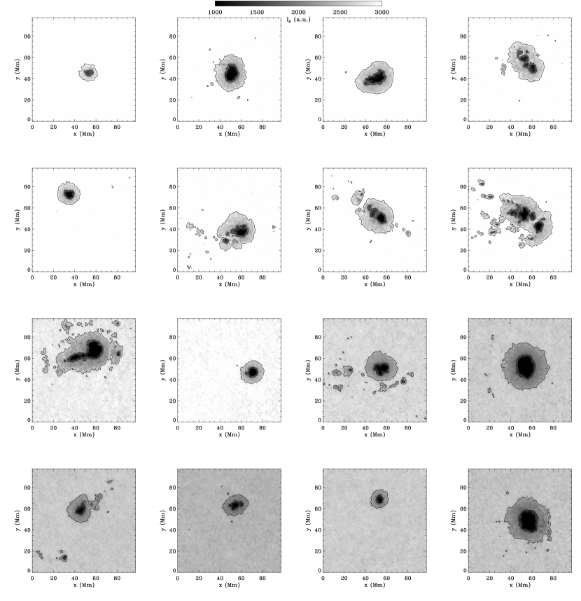
Figure 1: MDI continuum intensity of the 16 solar active regions studied in this paper, in the order listed in Table 1 (from the upper left to the lower right panel). The boundaries of the umbra and penumbra are overplotted: they correspond to $57\%$ and $85\%$ of the continuum intensity, respectively. The greyscale is the same for every panel.

For the purpose of this paper, a sunspot is defined as a group of contiguous pixels with a l.o.s magnetic field strength larger than 150 Gauss and that exhibits both an umbra and penumbra. The area of a spot is only the number of pixels within this spot multiplied by the area of a pixel $dx\times dy=0.682$ Mm². The l.o.s magnetic field flux is the value of $\mathbf{B}(\mathbf{r},0)$ at each pixel muliplied by the area of a pixel. Table 1 summarizes the properties of the active regions studied in this paper, while Figure 1 shows maps of their continuum intensity $I_{0}$.

2.2 Travel-Time Estimation

The time-distance formalism was introduced by Duvall et al. (1993). It is based on computation of cross-covariances between the solar oscillation signals at two locations on the solar surface (a source at $\mathbf{r_{1}}$ and a receiver at $\mathbf{r_{2}}$). Due to the stochastic excitation of acoustic waves by the solar convection zone and due to the oscillation signal at any location being a superposition of a large number of waves of different travel distances (i.e., of different horizontal phase velocities $v_{ph}=\omega/k$, where $k$ is the horizontal wavenumber and $\omega$ is the temporal angular frequency), the cross-covariances are very noisy and need to be phase-speed filtered and averaged (Duvall et al. 1997). The Doppler velocity data cube $\phi(\mathbf{r},t)$ is phase-speed filtered in the Fourier domain, using a Gaussian filter $F(k,\omega;\Delta)$ for each travel distance $\Delta$. The standard scheme of averaging is to average the point-to-point cross-covariances over an annulus of radius $\Delta=|\mathbf{r_{2}}-\mathbf{r_{1}}|$ centered on the source. Such point-to-annulus cross-covariances are computed for several distances $\Delta$ (55 in this paper), and then averaged by groups of 5 distances to further increase their signal-to-noise ratio. A detailed explanation of all these steps in the analysis process can be found in, e.g., Couvidat, Birch, & Kosovichev (2006), along with a table of distances $\Delta$ and phase-speed filter characteristics used (see Table 1 of previous reference).

The point-to-annulus cross-covariances are fitted by two Gabor wavelets (Kosovichev & Duvall 1997): one for the positive times, one for the negative times. We use the ingoing (i) and outgoing (o) phase travel times $\tau_{\mathrm{i/o}}(\mathbf{r},\Delta)$ returned by the fits. The average of these two travel times, $\tau_{\mathrm{mean}}(\mathbf{r},\Delta)$, is, in first approximation, sensitive only to the sound-speed $c(\mathbf{r},z)$ in the region of the Sun traversed by the wavepacket (where $z$ is the vertical coordinate). Using a solar model as a reference we can relate the mean travel-time perturbations $\delta\tau_{\mathrm{mean}}(\mathbf{r},\Delta)$ to the sound-speed perturbations $\delta c(\mathbf{r},z)$ through an integral relation:

$$\mathrm{\delta}\mathrm{\tau_{\mathrm{mean}}}(\mathbf{r},\mathrm{\Delta})=\int\!\!\!\!\int_{S}d\mathbf{r^{\prime}}\int_{-d}^{0}dz\,K(\mathbf{r}-\mathbf{r^{\prime}},z;\mathrm{\Delta})\,\frac{\mathrm{\delta}c^{2}}{c^{2}}(\mathbf{r^{\prime}},z)$$ (1)

where $S$ is the area of the region, and $d$ is its depth. The sensitivity kernel for the relative squared sound-speed perturbations is given by $K$. Here we use Born-approximation kernels kindly provided by A. C. Birch (Birch, Kosovichev, & Duvall 2004). These kernels take into account the finite wavelength effects of the wavefield. Equation 1 is only approximate because effects on the mean travel times other than the sound-speed perturbation are completely ignored. For instance, Bruggen & Spruit (2000) describe the impact of changes in the upper boundary condition in sunspots due to the Wilson depression; Woodard (1997) and Gizon & Birch (2002) demonstrate that increased wave damping in sunpots can introduce shifts in travel times; finally, the significant magnetic field effects, already mentioned in Introduction, also contribute to $\delta\tau_{\mathrm{mean}}(\mathbf{r},\Delta)$.

2.3 Inversion of Travel-Time Maps

Based on Equation 1 the mean travel-time perturbation maps (11 of them per datacube) are inverted for sound-speed perturbation using a regularized least-squares scheme based on a modified Multi-Channel Deconvolution algorithm (MCD; see Couvidat et al. 2005 for details on the modified algorithm, and Jacobsen et al. 1999 for the basic algorithm). The modified algorithm includes both horizontal and vertical regularizations. We use the weighted norm of, and that of the first derivatives of, the solution $\mathrm{\delta}c^{2}/c^{2}(\mathbf{r},z)$ for vertical and horizontal regularization, respectively. Following Couvidat et al. (2005) the covariance matrix of the noise in the travel-time maps is included in the inversion procedure, and is obtained by 40 realizations of noise travel-time maps based on the noise model by Gizon & Birch (2004). Both the horizontal and vertical regularization parameters are constant for the inversion of travel-time maps of all our datasets. These parameters are chosen empirically. We invert for 13 layers in depth, with the center of the deepest layer located $28.5$ Mm below the solar surface.

3 RESULTS AND DISCUSSION

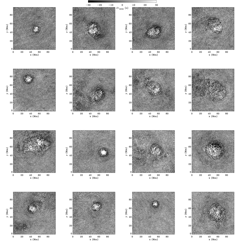
Figure 2: Mean travel-time perturbation maps $\delta\tau_{\mathrm{mean}}(\mathbf{r},\Delta)$ for the distance $\Delta=11.6$ Mm and for the 16 sunspots studied. The greyscale is the same for every panel and was truncated to emphasize the dark rings. The boundaries of the umbra and penumbra, as defined on Figure 1, are overplotted.

Figure 2 shows the mean travel-time perturbation maps for a travel distance $\Delta=11.6$ Mm over the 16 active regions. The main feature visible on most maps is a central white disk of increased travel times. Surrounding this disk, a dark ring corresponding to a decreased mean travel time is clearly present. Umbra and penumbra boundaries overplotted on Figure 2 show that this dark ring is mostly located within the penumbral region of the spot. Such dark rings actually appear in travel-time maps for 2 of the 11 distances $\Delta$ studied here: $\Delta=8.7$ Mm and $\Delta=11.6$ Mm. An azimuthal average of $\delta\tau_{\mathrm{mean}}(\mathbf{r},\Delta)$ around the sunspot center for 5 circular sunspots shows the average amplitude of the rings and their extent (see Figure 3). The rings do not seem to be present at $\Delta=6.2$ Mm; some spots exhibit them but most do not.

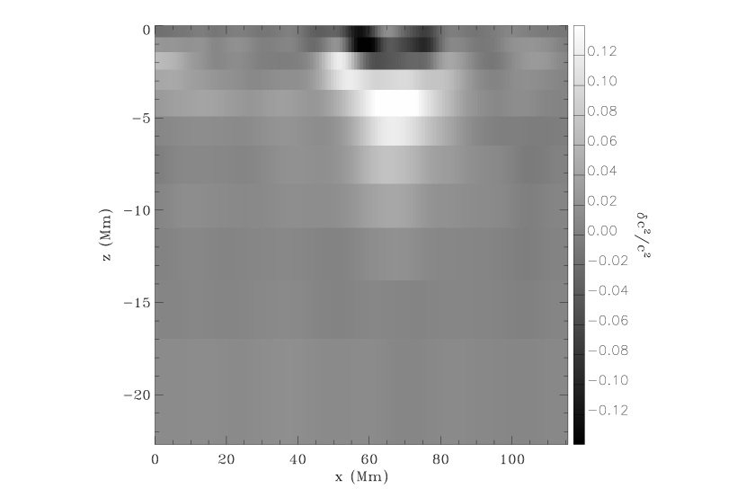
Figure 4: Vertical cut in the inverted sound-speed perturbation for the active region NOAA 8397.

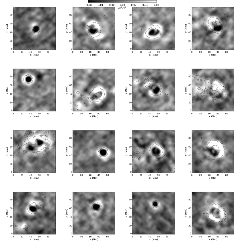
Figure 5: Inversion results $\delta c^{2}/c^{2}$: we show a horizontal cut at a depth of $z=-2.38$ to $z=-1.42$ Mm. The greyscale is the same for every panel and was truncated to emphasize the bright rings. The boundaries of the umbra and penumbra, as defined on Figure 1, are overplotted.

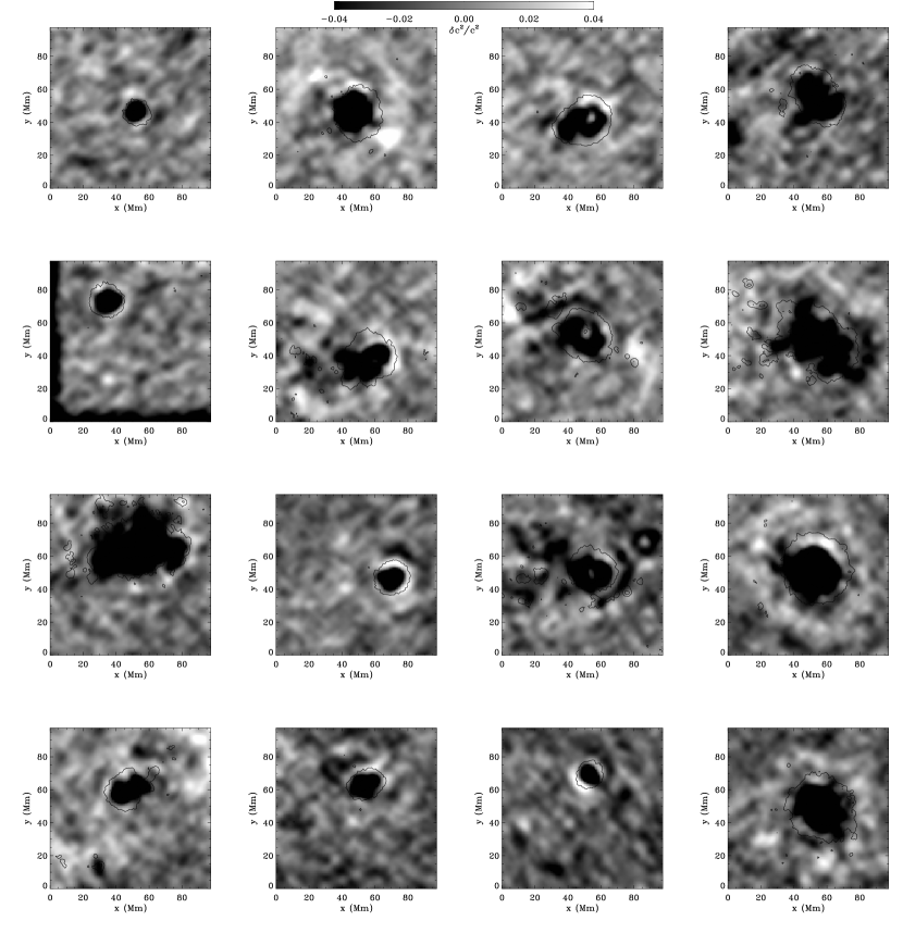
Figure 6: Inversion results $\delta c^{2}/c^{2}$: we show a horizontal cut at a depth of $z=-1.42$ to $z=-0.62$ Mm. The greyscale is the same for every panel and was truncated to emphasize the bright rings. The boundaries of the umbra and penumbra, as defined on Figure 1, are overplotted.

When travel-time maps are inverted for sound-speed perturbations, they produce the well known two-region structure below the active region: first the sound speed decreases just below the photosphere and then increases at a depth of about 3-4 Mm, depending on the sunspot size and magnetic flux. These two regions can be seen in Figure 4: this is a vertical cut in the inversion result for the active region NOAA 8397. The dark ring surrounding the corresponding sunspot on the travel-time maps of Figure 2 appears on Figure 4 as two bright arms extending from the region of increased sound-speed toward the surface. These arms are especially well visible at a depth of about $2$ Mm. Their amplitude decreases when we get closer to the solar surface. The rings/arms are not visible anymore at the surface, in agreement with the travel-time map at $\Delta=6.2$ Mm. Such ring-like/arm-like structures are present on most sunspots. Figure 5 shows horizontal cuts in the inversion results for the layer $z=-2.38$ to $z=-1.42$ Mm, while Figure 6 shows similar cuts for the layer $z=-1.42$ to $z=-0.62$ Mm.

An azimuthal average of the sound-speed perturbation for 5 circular sunspots as a function of the radial distance to the spot center is plotted on Figure 7, for the layers $z=-2.38$ to $z=-1.42$ Mm (upper panel) and $z=-1.42$ to $z=-0.62$ Mm (lower panel). At the layer $z=-2.38$ to $z=-1.42$ Mm, the averaged amplitude of the increased sound-speed region is always above the noise level on the inverted results, with a maximum value of about $\delta c^{2}/c^{2}=6\%$, corresponding to a sound-speed increase of about $0.45$ km s^-1. Neglecting the magnetic field influence, any change in the first adiabatic exponent, and any change in the mean molecular weight, we have $\delta c^{2}/c^{2}=\delta T/T$. Therefore, a $6\%$ increase in $\delta c^{2}/c^{2}$, translates into an upper limit for the temperature increase at $z=-1.9$ Mm of about $1100$ K. For the layer $z=-1.42$ to $z=-0.62$ Mm, the maximum value of the sound-speed perturbation for the 5 sunspots of Figure 7 is about $\delta c^{2}/c^{2}=2\%$ after azimuthal averaging, corresponding to an upper limit for the temperature increase of $295$ K.

It is worth mentioning that these ring-like/arm-like structures have already been detected in the past: for instance, Figure 4 of Hughes, Rajaguru, & Thompson (2005) clearly shows a ring on the inverted sound-speed perturbation map at $z=-2.3$ to $z=-1.7$ Mm. Their inversion was performed using ray-path approximation kernels, and the algorithm was LSQR and not the MCD used here. Another example is Figure 8 of Couvidat et al. (2004) which shows a clear ring structure around the sunspot NOAA 8243, after inversion with Fresnel-zone sensitivity kernels. The significance of these rings had been dismissed at that time.

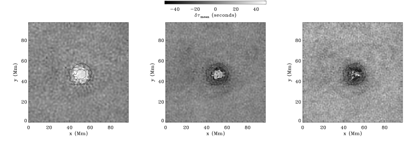
Figure 9: Travel-time maps $\delta\tau_{\mathrm{mean}}(\mathbf{r},\Delta)$ for the distance $\Delta=11.6$ Mm and the active Region NOAA 9493. Left panel: with a frequency filter centered on 3 mHz; central panel: filter centered on 4 mHz; right panel: filter centered on $4.5$ mHz. The greyscale is the same for all three panels.

To understand the nature of these rings —artifacts or real physical features— we perform several analyses. First, a recent study by Rajaguru et al. (2006) shows that the interaction of phase-speed filtering in time-distance analysis and the spatially localized p-mode amplitude reduction in sunspots introduces travel-time artifacts that are significant for short travel distances. To make sure that the rings we observe on the travel-time maps are not due to this p-mode amplitude effect, we applied the power correction suggested in their paper to a couple of sunspots: the dark ring is still present after correction, even though with a different size and a different amplitude. Figure 8 shows the impact of this correction: there might be a dependence on the sunpsot size; the dark ring being more affected by the power correction for small spots. Second, Braun & Birch (2006) observed frequency variations of solar p-mode travel times, using acoustic holography. They believe these variations are, at least partly, produced by surface effects due to magnetic fields. To test whether or not the dark rings have this frequency dependence, we followed Braun & Birch (2006) and computed some travel-time maps at $\Delta=11.6$ Mm with the same phase-speed filter but different temporal frequency filters: on top of the phase-speed filter $F(k,\omega;\Delta)$ we add a Gaussian $\nu=\omega/(2\pi)$ filter with a FWHM of $\delta\nu=1$ mHz and centered on different frequencies ($\nu=$3, 4, and $4.5$ mHz). The resulting travel-time maps for NOAA 9493 are shown in Figure 9: the size and amplitude of the ring clearly depend on the $\nu$ filter used. At low frequencies ($\nu$ filter centered on 3 mHz) the ring is almost non-existent, but as the frequency content of the wave-packets shifts to higher frequencies the ring broadens and its amplitude increases. At $4.5$ mHz, the ring extends inside the umbra and, maybe, even beyond the penumbra. Therefore, the near absence of rings on travel-time maps for $\Delta=6.2$ Mm might be partly due to the phase-speed filter we use at this distance: this filter selects wavepackets with a maximum power at about $\nu=3.5$ mHz. However, for $\Delta=11.6$ Mm, the selected wavepackets have a maximum power at about $4.25$ mHz. It should be noticed that with our frequency and broad phase-speed filters, selecting a specific frequency band also means selecting a slightly different average phase speed: both effects are entangled. Therefore what we consider to be a dependence on frequency might partly be a dependence on phase speed. Figure 9 also shows that the travel times in the umbra of the sunspot depend on frequency, albeit to a lesser extent than in the penumbra. Therefore, the rings might be the manifestation of a phenomenon affecting the entire spot, and directed from the periphery (the penumbra) to the center (the umbra) when the wave-packet frequency selected for the time-distance analysis is increased. Nevertheless, we do believe that the qualitative sound-speed inversion result below the umbra (two-region structure) holds, because the mean travel-time perturbation in the vicinity of the spot center is still consistently positive with the frequency filters applied for $\Delta=11.6$ Mm. However, this analysis undoubtedly confirms that the layers below a spot umbra have a lateral extent and an inverted $\delta c^{2}/c^{2}$ amplitude that depend on the wave-packet frequency. The problem seems less acute for deeper layers: the travel-time maps for larger distances $\Delta$ also vary with the frequency but no structure similar to the rings is ever present. Even though we suggest that the qualitative result of the sound-speed inversion below a sunspot is valid, any attempt to quantitatively assess the corresponding sound-speed perturbation amplitude and the lateral extent of the decreased sound-speed region are inextricably connected to the frequency band selected. Third, with the phase-speed filters (no frequency filter), we notice a strong asymmetry between ingoing and outgoing travel-time maps: the rings seem to be present only on the outgoing travel times (see Figure 10). This asymmetry might be an additional sign of an interaction of the wavefield with surface magnetic field (as suggested in, e.g, Lindsey & Braun 2005), but such a feature can also be explained by a flow (as first suggested by Duvall et al. 1996). Figure 10 shows that the ring appears both as partly due to a sound-speed perturbation (because it is visible on the mean travel-time maps), and as partly due to a flow if we accept the interpretation of Duvall et al. (1996) (because it is visible on the difference travel-time maps). The sign of $\delta\tau_{\mathrm{o}}-\delta\tau_{\mathrm{i}}$ at $\Delta=11.6$ Mm points to an inflow below the spot umbra, and an outflow in the penumbral ring. Such a reversal in the flow direction seems physically implausible. Finally, Figure 11 shows a loose dependence of the maximum sound-speed perturbation in these rings at a depth of $z=-2.38$ to $z=-1.42$ Mm as a function of the total magnetic flux of the sunspot: the larger the magnetic flux or the sunspot size (Table 1 shows a linear relation between these two parameters), the larger is $\delta c^{2}/c^{2}$ in the arms/rings. This last observation is inconclusive though because the subsurface structure of the spot might also depend on the total flux: it does not help in discriminating between the ring-as-artifact and the ring-as-real-structure hypotheses.

Considering that the rings are located mainly below the sunspot penumbra in the inversion results and inside the penumbra on the travel-time maps, that there is a strong asymmetry between ingoing and outgoing travel-time maps (with rings present only on the outgoing travel times), and that the ring size and amplitude have a very clear frequency dependence, it seems hard to believe that the sound-speed increase they imply is the signature of a real solar feature located in depth. Indeed it seems more likely that these rings are spurious features produced by frequency dependent surface effects somewhat related to the strong magnetic field of the sunspots, which are not accounted for in the inversion procedure.

4 CONCLUSION

We clearly detect rings of negative mean travel-time perturbations on the travel-time maps of most sunspots for travel distances between $\Delta=8.7$ and $\Delta=11.6$ Mm. These rings produce significant arm-like/ring-like structures on the inversion results, mimicking regions of increased sound speed. However due to the locations of these structures (immediately below the sunspot penumbrae), and their sensitivity to the filtering applied to the Doppler velocity datacubes, it is likely that they are artifacts produced by the interaction of the wavefield and surface magnetic fields. These significant structures were not mentioned in the paper by Zhao & Kosovichev (2006). Even though we agree with their conclusion that the effect of the surface magnetic field probably does not change the qualitative inversion result of the basic sunspot structure (the two-region structure), we show that these inversion results for the first 3-4 Mm below the solar surface appear to be significantly contaminated by surface effects probably of magnetic origin. Indeed, the rings could be the most visible manifestation of a general phenomenon that also affects the amplitude and the lateral extent of the sound-speed perturbation in the shallower subsurface layers.

Table 1: Characteristics of the Sunspots Studied, for a Threshold of 150 G

NOAA	Date	Area	Flux	Class	lat.	long.	Index
8073	08.17.1997	229.25	129897	$\alpha$	14.5	282.0	40553
8243	06.18.1998	694.59	455180	$\beta$	18.3	214.5	47871
8397	12.04.1998	745.76	492968	$\beta$	16.5	140.6	51932
8402	12.05.1998	298.17	187218	$\beta$	17.0	122.5	51958
8402	12.07.1998	788.06	436916	$\beta$	16.8	121.8	51983
8602	06.29.1999	867.21	543457	$\beta$	19.1	298.7	56893
8742	10.30.1999	796.93	527631	$\beta$	7.0	121.0	59829
8760	11.10.1999	1677.79	1019900	$\beta$	13.0	330.0	60102
9236	11.24.2000	1849.05	1062150	$\beta$	18.5	359.0	69216
9493	06.12.2001	311.13	202267	$\beta$	5.8	235.2	74032
0061	08.09.2002	576.55	363652	$\beta-\delta$	8.5	45.2	84183
0330	04.09.2003	1288.19	819593	$\beta-\gamma$	6.2	82.2	90015
0387	06.23.2003	617.49	335377	$\beta-\gamma$	17.0	166.5	91806
0615	05.21.2004	404.61	216729	$\alpha$	15.6	93.7	99812
0689	10.27.2004	206.06	114991	$\alpha$	9.7	155.0	103621
0898	07.03.2006	1194.03	699494	$\beta$	-5.5	329.0	118363

Figure 3: Azimuthal average of $\delta\tau_{\mathrm{mean}}(\mathbf{r},\Delta)$ for $\Delta=6.2$ Mm (upper panel), $\Delta=8.7$ Mm (second panel from the top), and $\Delta=11.6$ Mm (third panel) and for 5 sunspots: NOAA 9493 (solid line), 8073 (short-dashed line), 0615 (dot-dashed line), 8402 (dot-dot-dot-dashed line), and 0689 (long-dashed line). The lower panel shows an azimuthal average of the normalized continuum intensity.

Figure 7: Azimuthal averages of the inverted sound-speed perturbation at a depth of $z=-2.38$ to $z=-1.42$ Mm (upper panel) and $z=-1.42$ to $z=-0.62$ Mm (lower panel), as a function of the radial distance to the spot center, for 5 sunspots: ARs 9493 (solid line), 8073 (short-dashed line), 0615 (dot-dashed line), 8402 (dot-dot-dot-dashed line), and 0689 (long-dashed line).

Figure 8: Upper panel: azimuthal average of $\delta\tau_{\mathrm{mean}}(\mathbf{r},\Delta)$ for the distance $\Delta=11.6$ Mm and the active Region NOAA 8397. The solid line is before the power correction of Rajaguru et al. (2006), the dashed line is after correction. Lower panel: same plot for the active region NOAA 8073.

Figure 10: Azimuthal average of $\delta\tau_{\mathrm{o}}(\mathbf{r},\Delta)$ (outgoing travel times; upper panel) and $\delta\tau_{\mathrm{i}}(\mathbf{r},\Delta)$ (ingoing travel times; lower panel) for $\Delta=11.6$ Mm and for 5 sunspots: NOAA 9493 (solid line), 8073 (short-dashed line), 0615 (dot-dashed line), 8402 (dot-dot-dot-dashed line), and 0689 (long-dashed line).

Figure 11: Maximum value of the sound-speed perturbations in the rings surrounding the spots for the layer $z=-2.38$ to $z=-1.42$ Mm, as a function of the sunspot magnetic flux (see Table 1). The error bars are $\pm$ the rms variation of the inverted sound-speed perturbations at the selected layer. The solid line is the result of a linear fit.

References

- Birch et al. (2004) Birch, A. C., Kosovichev, A. G., & Duvall, T. L., Jr. 2004, ApJ, 608, 580
- Braun & Lindsey (2000) Braun, D. C., & Lindsey, C. 2000, Sol. Phys., 192, 307
- Braun & Birch (2006) Braun, D. C., & Birch, A. C. 2006, ApJ, 647, L187
- Bruggen & Spruit (2000) Bruggen, M., & Spruit, H. C. 2000, Sol. Phys., 196, 29
- Cally et al. (2003) Cally, P. S., Crouch, A. D., & Braun, D. C. 2003, MNRAS, 346, 381
- Couvidat et al. (2004) Couvidat, S., Birch, A. C., Kosovichev, A. G., & Zhao, J. 2004, ApJ, 607, 554
- Couvidat et al. (2005) Couvidat, S., Gizon, L., Birch, A. C., Larsen, R. M., & Kosovichev, A. G. 2005, ApJS, 158, 217
- Couvidat et al. (2006) Couvidat, S., Birch, A. C., & Kosovichev, A. G. 2006, ApJ, 640, 516
- Duvall et al. (1993) Duvall, T. L., Jr., Jefferies, S. M., Harvey, J. W., & Pomerantz, M. A. 1993, Nature, 362, 430
- Duvall et al. (1996) Duvall, T. L., Jr., D’Silva, S., Jefferies, S. M., Harvey, J. W., & Schou, J. 1996, Nature, 379, 235
- Duvall et al. (1997) Duvall, T. L., Jr. et al. 1997, Sol. Phys., 170, 63
- Gizon & Birch (2002) Gizon, L., & Birch, A. C. 2002, ApJ, 571, 966
- Gizon & Birch (2004) Gizon, L., & Birch, A. C. 2004, ApJ, 614, 472
- Haber et al. (2002) Haber, D. A., Hindman, B. W., Toomre, J., Bogart, R. S., Larsen, R. M., & Hill, F. 2002, ApJ, 570, 855
- Hughes et al. (2005) Hughes, S. J., Rajaguru, S. P., & Thompson, M. J. 2005, ApJ, 627, 1040
- Jacobsen et al. (1999) Jacobsen, B. H., Mller, I., Jensen, J. M., & Effers, F. 1999, Phys. Chem. Earth, 24, 15
- Kosovichev et al. (1997) Kosovichev, A. G., & Duvall, T. L., Jr. 1997, Proceedings of SCORe’96 : Solar Convection and Oscillations and their Relationship, Eds.: F.P. Pijpers, J. Christensen-Dalsgaard, and C.S. Rosenthal, Kluwer Academic Publishers (Astrophysics and Space Science Library Vol. 225), 241
- Kosovichev et al. (2000) Kosovichev, A. G., Duvall, T. L., Jr., & Scherrer, P. H. 2000, Sol. Phys., 192, 159
- Lindsey & Braun (2005) Lindsey, C., & Braun, D. C. 2005, ApJ, 620, 1107
- Liu et al. (2007) Liu, Y., Norton, A. A., & Scherrer, P. H. 2007, Sol. Phys., accepted
- Rajaguru et al. (2006) Rajaguru, S. P., Birch, A. C., Duvall, T. L., Jr., Thompson, M. J., & Zhao, J. 2006, ApJ, 646, 543
- Rajaguru et al. (2007) Rajaguru, S. P., Sankarasubramanian, K., Wachter, R., & Scherrer, P. H. 2007, ApJ, 654, L175
- Scherrer et al. (1995) Scherrer, P. H., et al. 1995, Sol. Phys., 162, 129
- Schunker et al. (2005) Schunker, H, Braun, D. C., Cally, P. S., & Lindsey, C. 2005, ApJ, 621, L149
- Schunker & Cally (2006) Schunker, H., & Cally, P. S. 2006, MNRAS, 372, 551
- Woodard (1997) Woodard, M. F. 1997, ApJ, 485, 890
- Zhao et al. (2001) Zhao, J., Kosovichev, A. G., & Duvall, T. L., Jr. 2001, ApJ, 557, 384
- Zhao et al. (2006) Zhao, J., & Kosovichev, A. G. 2006, ApJ, 643, 1317