An Observational Limit on the Earliest GRBs

Abstract

We predict the redshift of the first observable (i.e., in our past light cone) Gamma Ray Burst (GRB) and calculate the GRB-rate redshift distribution of the Population III stars at very early times ($z=20-60$). Using the last 2 years of data from Swift we place an upper limit on the efficiency ($\eta_{GRB}$) of GRB production per solar mass from the first generation of stars. We find that the first observable GRB is most likely to have formed at redshift 60. The observed rate of extremely high redshift GRBs (XRGs) is a subset of a group of 15 long GRBs per year, with no associated redshift and no optical afterglow counterparts, detected by Swift. Taking this maximal rate we get that $\eta_{GRB}<1.1~{}10^{-4}$ GRBs per solar mass in stars. A more realistic evaluation, e.g., taking a subgroup of $5\%$ of the total sample of Swift gives an upper limit of $\eta_{GRB}<3.2~{}10^{-5}$ GRBs per solar mass.

1 Introduction

Gamma Ray Bursts (GRBs) are the brightest known events since the Big Bang (see reviews by: Piran, 2005, 2000; Mészáros, 2002). Therefore they offer a wonderful prospect to explore the evolution of the Universe ever since stars began to form. The first generation of stars is expected to be massive (Abel et al., 2002; Bromm, Coppi, & Larson, 2002), and at least some of them should form a GRB as they end their lives (e.g., Heger et al., 2003). Since the luminosities of galaxies and quasars decline with redshift, high redshift GRBs are expected to be easier to observe than their host galaxies. Consequently, they can offer a significant probe of the early universe (e.g., Lamb & Reichart, 2000). For example, since the GRB afterglows fade only slowly with redshift they offer a source for studying the cosmic reionization (Barkana & Loeb, 2004, 2006). In particular, GRBs formation history is expected to follow the star formation evolution (Blain & Natarajan, 2000; Porciani & Madau, 2001).

The first stars in the Universe namely, population III (POP III), formed at very high redshift ($z\lower 2.15277pt\hbox{$\;\buildrel<\over{\sim}\;$}66$, Naoz, Noter & Barkana, 2006). Since metals are absent in the pre-stellar universe, the earliest available coolant is molecular hydrogen (H₂). Thus the minimum halo mass that can form a star is essentially set by requiring the infalling gas to reach a temperature $>1000$ K required for exciting the rotational and vibrational states of molecular hydrogen (Tegmark, 1997). Numerical simulations (Abel et al., 2002; Fuller & Couchman,, 2000; Yoshida, et al., 2003; Reed et al., 2005; Bromm, Coppi, & Larson, 2002) give a more accurate constraint and require a minimum circular velocity $V_{c}\sim 4.5$ km/s, where $V_{c}=\sqrt{GM/R}$ in terms of the halo virial radius $R$. These simulations include gravity, hydrodynamic and chemical processes in the primordial gas, and show that the first star formed within a galactic halo of $\sim 10^{5}M_{\odot}$ in total mass. The predicted mass of this star is quite heavy and should exceed $100M_{\odot}$ (Yoshida et al., 2006; Gao et al., 2007).

The radiation from these first stars is expected to eventually dissociate all the $H_{2}$ in the intergalactic medium, leading to the domination of a second generation of larger galaxies where the gas cools via radiative transitions in atomic hydrogen and helium (Haiman et al., 1997). Atomic cooling occurs in halos with $V_{c}>16.5$ km/s, in which the infalling gas is heated above 10,000 K and is ionized.

Bromm & Loeb (2006) calculated the star formation evolution for population III while assuming only atomic cooling in order to derive the GRB rate. They assumed that the efficiency of GRB production ($\eta_{GRB}$) is $\sim 10^{-9}$ GRBs per solar mass in stars, and found that about $10\%$ of all bursts detected by Swift should be generated from redshift $\geq 5$. Unlike these writers and GRB rate analysis done by others (e.g., Guetta, Piran, & Waxman, 2005; Guetta & Piran, 2005, 2007; Bromm & Loeb, 2002, 2006; Daigne, Rossi, & Mochkovitch, 2006, and references therein), we concentrate on a much higher redshift regime ($z=20-60$) and we estimate the upper bound of the efficiency of extremely high redshift GRBs (XRGs) production. The article is structured as follow: we begin by presenting a simple star formation evolution (Section 2), relevant for these redshifts. Our analysis is presented in Section 3. In Section 3.1 we calculate the redshift of the first observable GRB. Section 3.2 is dedicated to the calculation of the redshift distribution of the XRG rate, in order to place an upper limit on $\eta_{GRB}$. We conclude with a discussion of our results (Section 4).

Our calculations are made in a $\Lambda$CDM universe, including dark matter, baryons, radiation, and a cosmological constant. We assume cosmological parameters matching the three year WMAP data together with weak lensing observations (Spergel et al., 2006), i.e., $\sigma_{8}=0.826$, $\Omega_{m}=0.299$, $\Omega_{\Lambda}=0.74$, and $\Omega_{b}=0.0478$.

2 Estimation of the High Redshift Star Formation Rate

We adopt a simple model for the star formation history at high redshift ($z\sim 70-20$). This modle assumes that at these early times most of the stars formed out of newly accreted gas during mergers. We follow the linear and non linear perturbation growth from Naoz & Barkana (2005) and Naoz, Noter & Barkana (2006) in order to derive the fraction of mass in halos.

Naoz & Barkana (2005) showed that the baryon sound speed varies spatially, so that the baryon temperature and linear density fluctuations must be tracked separately. In the non-linear regime, it is necessary to calculate correctly the linearly extrapolated overdensity $\delta_{c}$ which marks the time of the collapse. Naoz, Noter & Barkana (2006) showed that the value of $\delta_{c}$ is lower at high redshift than the classical value ($1.686$) and varies with time (see for reference fig. 6 in Naoz & Barkana, 2007). Defining the mass variance $S=\sigma^{2}(M,z)$, we calculate the Sheth & Tormen (2001) mass function, which fits simulations and includes non-spherical effects on the collapse. The function $f_{ST}$ is the fraction of mass associated with halos of mass $M$:

$$f_{ST}(\delta_{c},S)=A^{\prime}\frac{\nu}{S}\sqrt{\frac{a^{\prime}}{2\pi}}\left[1+\frac{1}{\left(a^{\prime}\nu^{2}\right)^{q^{\prime}}}\right]\exp\left[\frac{-a^{\prime}\nu^{2}}{2}\right]\ ,$$ (1)

where $\nu=\delta_{c}/\sqrt{S}$. We use best-fit parameters $a^{\prime}=0.75$ and $q^{\prime}=0.3$ (Sheth & Tormen, 2002), and ensure normalization to unity by taking $A^{\prime}=0.322$. We apply this formula with $\delta_{c}(z)$ and $\sigma^{2}(M,z)$ as the arguments.

As mentioned, the only coolant available for these high redshift halos is cooling via H₂  cooling. Thus, we find the fraction of mass in halos with mass larger than the minimum H₂  cooling mass to be

$$F(>M_{min,H_{2}}(z))=\int{f_{ST}(\delta_{c}(z),S)dS}\ .$$ (2)

Thus the star formation rate (SFR) (based on H₂  cooling) is simply:

$$SFR=\frac{dF}{dt}\rho_{0}\frac{\Omega_{b}}{\Omega_{m}}\epsilon\ ,$$ (3)

where $\rho_{0}$ is the comoving matter density, and $\epsilon$ is the star formation efficiency. Barkana & Loeb (2000) calculated the star formation history for lower redshifts using a more complicated calculation that included additional merger-induced star formation. Bromm & Loeb (2006) have calculated separately the star formation rate for the different star populations, i.e., POP I/II and POP III. In both papers the star formation efficiency was chosen to be $10\%$ independent of redshift. This yields a rough agreement between the SFR at low redshift and the observations (see fig. 1 in Barkana & Loeb, 2000). Following these previous analyses we set $\epsilon=10\%$.

In figure 1 we plot the SFR as a function of $1+z$ as derived from eq. 3. We note that this result is very close to that obtained by Bromm & Loeb (2002, 2006) for the star formation of POP III. However our result predicts a higher rate because we consider star formation at higher redshifts. In practice our result is between their most optimistic (high efficiency) estimate and their most pessimistic case. In addition our simple model does not include the radiation feedback which lowers the contribution of molecular hydrogen cooling compared to atomic cooling (see for reference Haiman et al., 1997; Barkana & Loeb, 2001). Therefore we restrict ourselves to all redshifts $\geq 20$ (note that the redshift range considered by Bromm & Loeb (2006) is $z\lower 2.15277pt\hbox{$\;\buildrel<\over{\sim}\;$}30$). Since we do not account for reionization effects at all we compare our results to that of a late reionization in (figure 1 top panel in Bromm & Loeb, 2006).

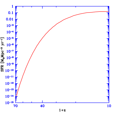
Figure 1: Redshift evolution of SFR in halos larger than the minimum H₂  cooling mass, in $M_{\odot}$ yr^-1 per comoving Mpc³. This is the prediction from the model presented in equation 3.

3 Calculations and results

In order to produce a GRB the progenitor must fulfill 3 requirements (see Zhang, Woosley, & Heger, 2004; Petrovic et al., 2005; Bromm & Loeb, 2006, for more detailed explanation). First, the star must be massive enough to result in a black hole. Second, the star must lose its hydrogen envelope in order to allow the relativistic jet to penetrate through the surface (Zhang, Woosley, & Heger, 2004), and finally an accretion disk must be able to form. For that the star must maintain enough angular momentum. When evaluating the efficiency of producing GRBs from POP III stars there are many uncertainties, such as the properties of the progenitor. Bromm & Loeb (2006), for example, claim that in order to produce a GRB, the progenitor must have a close binary companion that helps in stripping the hydrogen envelope and retaining sufficient angular momentum in the collapsing core. However, Fryer, Woosley, & Heger (2001) show that massive POP III stars can produce pair-instability supernovae that can strip off their hydrogen envelope and result in a black hole accretion disk system. Heger et al. (2003) deploy a variety of masses that can produce GRBs from single POP III stars. Whether or not binary stars are a strict requirement for GRB production is still debatable. However, our analysis is independent of that question. We only assume that GRBs in this high redshift regime do exist, and use observational constrains to extract the efficiency of producing them.

The most naive assumption is that each star (or binary system) at the relevant high redshift range produces a GRB and thus $\eta_{GRB}\sim 1/100$ GRBs per solar mass (or $1/200$ assuming binary progenitors). We derive further restrictions on $\eta_{GRB}$ by normalizing the GRB rate with the potential XRG rate observed by Swift (see text below for details).

3.1 The First Observable GRB

Naoz, Noter & Barkana (2006) have found that the first star most likely formed at $z=65.8$. As mentioned above, this star is expected to have a mass $\lower 2.15277pt\hbox{$\;\buildrel>\over{\sim}\;$}100~{}M_{\odot}$ (Abel et al., 2002), thus it (as well as the stars that follow it) is a suitable candidate to produce a GRB (Heger et al., 2003). We assume that GRBs at these redshifts are bright enough to be observed today (estimates of the limiting luminosity are given below using a more complex model), and adopt a fiducial jet opening angle of $5^{\circ}$ (e.g., Frail et al., 2001). This limited opening angle means that we see only two out of $500$ GRBs. The probability to observe the first GRB on the sky is computed following Naoz, Noter & Barkana (2006) analysis for the formation of the first star. Notice that since the lifetime of the first stars is insignificant compared to the Hubble time, we can neglect the delay time between the star formation and explosion. We find that most likely the first observable GRB is formed at $z=59.9$, with a $1$-$\sigma$ ($68\%$) range of $z=58.9$–61.4 and a $2$-$\sigma$ ($95\%$) range of $z=58.1$–63.5. Note that the most probable redshift of the first GRB is only weakly sensitive to changing the opening angle. For example an isotropic GRB will be seen at the redshift of the first observable star. $20^{\circ}$ we find that Considering an opening angle of $5^{\circ}$ we place an upper redshift limit for observing GRBs. Combining with the limitation of our SFR model we concentrate on the redshift range of: $20-60$.

3.2 GRB production efficiency and rate

From equation (3) we can evaluate the observable GRB rate:

$$R_{GRB}(z)=\eta_{GRB}\frac{SFR}{1+z}\frac{dV}{dz}\int_{L_{min}(z)}^{\infty}\phi(L)d\log L\ ,$$ (4)

where $V$ is the comoving volume and the factor $(1+z)^{-1}$ accounts for the cosmological time dilation. $\eta_{GRB}$ was defined earlier as the GRB efficiency in units of GRBs per solar mass, and $\phi(L)$ is the GRB luminosity function. The limiting luminosity at a given redshift, $L_{min}$, depends on the flux sensitivity threshold of the detector ($f_{lim}$), and can be written as:

$$L_{min}=4\pi d_{L}^{2}(z)f_{lim}\bigg{\{}\frac{C(E1(1+z),E2(1+z))}{C(E1,E2)}\bigg{\}}^{-1}\ ,$$ (5)

where $d_{L}(z)$ is the luminosity distance and C(E1,E2) is the total integrated luminosity for observation with Swift between $E1=50$ and $E2=300$ keV (for specific explanation see for reference Guetta & Piran, 2007; Schmidt, 1999).

Assuming an average photon number distribution of a single power law, eq. (5) can be written as (see for reference: Schmidt, 2001):

$$L_{min}=4\pi d_{L}^{2}(z)f_{lim}(1+z)^{-(2+\bar{\alpha})}\ .$$ (6)

where $\bar{\alpha}$ is the average photon spectral index over the energy range (i.e., $dN/dE\propto E^{\bar{\alpha}}$, where $N$ is the number of photons). A typical GRB photon number distribution can be described as a broken power law, also known as a Band spectrum (Band et al., 1993). The low energy regime has a spectral slope of $\alpha\simeq-0.8$, while the high energy regime has a slope of $\beta\simeq-2.5$ (Preece et al., 2000). The peak energy ($E_{p}$) falls in the range of 100 keV to a few MeV, which renders it observable by Swift.

Several groups (e.g., Yonetoku et al., 2004; Ghirlanda et al., 2005; Lamb, Donaghy, & Graziani, 2005) using various samples taken from BATSE, BeppoSax, Integral and HETE2, found that $E_{p}\sim L_{iso}^{0.5}$, where $L_{iso}$ is the GRB isotropic equivalent luminosity (either average or peak luminosity). Each burst that has an $E_{p}$ which falls within our observation window, can be fitted with an average photon spectral slope, $-0.8\lower 2.15277pt\hbox{$\;\buildrel<\over{\sim}\;$}\bar{\alpha}\lower 2.15277pt\hbox{$\;\buildrel<\over{\sim}\;$}-2.5$. Because $E_{p}$ is the break energy in the power law and bursts with higher luminosity have higher $E_{p}$, the average observed slope of such bursts should be higher (i.e., shallower) as well. Schmidt (2001) found for a sample of simulated long GRBs a median value of $\bar{\alpha}=-1.6$. In addition he found a positive correlation between $\bar{\alpha}$ and the GRB luminosity, as expected from the $E_{p}$-$L_{iso}$ relation. For example a typical XRG, at $z=20$, with an intrinsic luminosity of $10^{53}~{}$erg sec^-1 has an $E_{p}\sim 1~{}$MeV which will be redshifted to $\sim 50~{}$keV. The photon spectrum within the BAT observational window will have an average spectral slope of $\bar{\alpha}\simeq-1.6$.

We use this single power law to get a simplified k-correction for our bursts, where we expect most XRG spectral slopes to fall between $-1.6$ and $-1$, since their luminosity is in the high tail of the luminosity function. We adopt a limiting case of $\bar{\alpha}=-1$, according to the Schmidt (2001) hardness luminosity correlation. We also address the difference that adopting the median value ($-1.6$) would make in our results.

Lamb & Reichart (2000) assumed that the Swift threshold limit would be $f_{lim}=0.04$ photons cm^-2 sec^-1, and that the spectral photon index is $-1$. For an observed photon number flux with an observed redshift they found the luminosity of the burst as well as the maximum observable redshift. For example, for burst GRB971214 they found a peak luminosity of $6.4\times 10^{58}$ sec^-1, and showed that a burst with this luminosity can be seen up to redshift $\sim 70$. Repeating this exercise with the 2-year Swift threshold limit $f_{lim}=0.2$ photons cm^-2 sec^-1 we find that a burst with this peak luminosity can be seen at least up to $z\sim 21$, while adopting $\bar{\alpha}=-1.6$ yields a maximum observable redshift of $7.8$. Thus, the maximum observed redshift for a given luminosity is dependent on the spectral index.

In figure 2 we plot the maximum observable redshift of a burst as a function of the spectral index, for three different representative luminosities, from bottom to top: $10^{51},10^{52}$ and $10^{53}$ ergs sec^-1. The figure is plotted for $f_{lim}=0.2$ photons cm^-2 sec^-1, and it can be seen that the maximum observable redshift of a fixed luminosity GRB is strongly dependent on the spectral index. Note that high luminosity bursts are observable to higher redshift, especially since they tend to have high $\bar{\alpha}$. In the figure we indicate the limiting value and the median value of $\bar{\alpha}$ , $-1$ and $-1.6$, respectively. Thus, high luminosity bursts ($\sim 10^{53}$ ergs sec^-1) with $\bar{\alpha}\sim-1$ can be expected to be observed up to $z\sim 80$, while for the median value of the spectral index $-1.6$ the bursts are expected to be observed up to $z\sim 18$. Thus observing GRBs from a higher redshift (while assuming $\bar{\alpha}=-1.6$) suggests much more luminous bursts than $\sim 10^{53}$ ergs sec^-1. Of course this can also mean (when placing an upper limit on the luminosity) that there are no observable extremely high redshift GRBs with the current Swift detection limit. Therefore for Swift to detect XRGs, their average spectral slope should be closer to $-1$, as shown in fig. 2.

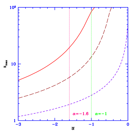
Figure 2: The maximum detectable redshift by Swift as a function of the spectral photon index $\bar{\alpha}$, using the Swift detection threshold $f_{lim}=0.2$ photons cm^-2 sec^-1. We consider three representative luminosities. From bottom to top: $10^{51},10^{52}$ and $10^{53}$ ergs sec^-1. Also shown are the median spectral index value from Schmidt (2001), $\bar{\alpha}=-1.6$ and the limiting case $\bar{\alpha}=-1$.

We assume the Guetta, Piran, & Waxman (2005) and Guetta & Piran (2007) luminosity function based on Schmidt (2001). This luminosity function has a broken power law with cutoff luminosities of $L^{\star}/\Delta_{1}$ and $\Delta_{2}L^{\star}$.

$$\phi(L)=c_{0}\left\{\begin{array}[]{ll}\left(\frac{L}{L^{\star}}\right)^{a}&\frac{L^{\star}}{\Delta_{1}}<L<L^{\star}\ ,\\ \left(\frac{L}{L^{\star}}\right)^{b}&L^{\star}<L<\Delta_{2}L^{\star}\ ,\\ \end{array}\right.$$ (7)

where $\phi(L)$ is normalized so that the integral over the luminosity function equals unity through $c_{0}$. We have used the Guetta & Piran (2007) best fitted values with $\Delta_{1},\Delta_{2}=100$, $L^{\star}=6.5\times 10^{51}$ erg sec^-1, $a=-0.2$ and $b=-1.7$, marked in their paper as model (v). This model favors high luminosity bursts, which are the interesting case here. We also address their (vi) model with $b=-2$ which has fewer high luminosity bursts (see text below).

We can now return to eq. (4) and calculate the XRG rate from POP III stars at $z=60-20$, and use that to place an upper limit of the efficiency of GRB production from these stars. We ask what is the efficiency of GRB production assuming that Swift observes up to $\sim 15$ long GRBs per year originating from these high redshift POP III stars. This subsample includes GRBs with no associated redshift (there are about 60 per year out of 90 per year). In addition we exclude GRBs with $T_{90}$ shorter than $50~{}$sec, where $T_{90}$ defines the duration of the burst, since short GRBs most likely originate from much lower redshift (see for reference: Nakar, 2006). Finally we exclude GRBs with no optical counterparts for the following reason: consider a burst at $z\sim 20$, with an afterglow counterpart. The photons of the burst redshift with the expansion of the Universe as they propagate. Wavelengths shorter than the Lyman limit will be absorbed by photoionizing hydrogen or helium atoms. Assuming that the Universe was completely reionized at $z\sim 10$ or later each $z=0$ optical photon was at a wavelength shorter than the Lyman limit and thus was absorbed in the pre-reionization era (see for reference: Barkana & Loeb, 2001). Therefore, no optical afterglow should be observed from XRGs, and we are left with about 15 bursts per year from the Swift sample. Of course assuming that all of this sample originates from high redshift is mostlikely an overestimate. Nevertheless, it gives an upper limit to the efficiency. Below we give more realistic estimates of the XRG rate detected by Swift.

In figure 3 top panel, we depicted the predicted GRB rate redshift distribution for various efficiency normalizations. We consider both cases of $\bar{\alpha}=-1$ (solid curves) as well as $\bar{\alpha}=-1.6$ (dashed curves). For the first case we consider XRGs that contribute (from top to bottom) $15,5$ and $1$ GRBs per year to the total sample detected by Swift. The GRB efficiencies from these values are: $\eta_{GRB}=1.1~{}10^{-4}$,$3.5~{}10^{-5}$ and $7.1~{}10^{-6}$ GRBs per solar mass, respectively. For the latter case ($\bar{\alpha}=-1.6$) we consider the same contributions, (top to bottom) $15,5$ and $1$ GRBs per year from the relevant redshift. The resulting upper limit on the efficiency is $\eta_{GRB}=2.6~{}10^{-3},8.7~{}10^{-4}$ and $1.7~{}10^{-4}$ GRBs per solar mass, respectively. Not presented in the figure is the lower limit case of $\bar{\alpha}=-2.2$. We find that for this spectral index Swift will be able to detect only a few GRBs per year. Comparing with the results above, in this case the efficiency needed to contribute one GRBs per year detectable by Swift is $4.2~{}10^{-3}$ GRBs per solar mass.

As can be seen from the figure in order to generate the same contribution of GRBs per year, the efficiency must be different for different spectral indices. Adopting $\bar{\alpha}=-1$ generates a lower efficiency for the same percentage of GRB contribution. This can be seen more clearly in the bottom panel of this figure, where we depict the GRB efficiency per solar mass ($\eta_{GRB}$) for various fractional contribution of GRBs from redshifts $20-60$ (out of $\sim 90$ GRBs per year detected by Swift). We consider the spectral index of $-1$ (solid curve) and also spectral index of $-1.6$ (dashed curve). For example, for a $1\%$ contribution of GRBs detected by Swift per year from this redshift range, i.e., about one GRB per year, we find that a spectral index of $-1$ predicts about $2$ orders of magnitude lower efficiency of GRB production than assuming a spectral index of $-1.6$. As mentioned before, the latter spectral index suggests much more luminous GRBs which is less reasonable. We also consider (in this bottom panel of figure 3) the parameters of model (vi) in Guetta & Piran (2007) (doted curve), which is less favorable for high luminosity bursts ($b=-2$). As can be expected this model results in a higher GRB efficiency since the luminosity function does not favor high luminosity bursts.

Bromm & Loeb (2006) found that about $10\%$ of the GRBs detected by Swift each year should result from high redshift ($\geq 5$) stars. However they assumed a lognormal luminosity function, and efficiency of $\sim 10^{-9}$ GRBs per solar mass. Thus if this $10\%$ claim is true, it is reasonable to assume that even less originate from a higher redshift ($\geq 20$) range. Suppose we assume a more reasonable upper limit for example, about $5\%$ to the total sample (about half of their range) . Using their luminosity function (see eq. 8 in Bromm & Loeb, 2002) we find that for $\bar{\alpha}=-1$, this $5\%$ contribution (about five GRBs per year) results in an upper limit on the efficiency of: $1.8~{}10^{-6}$ GRBs per solar mass, while assuming $\bar{\alpha}=-1.6$ gives an efficiency of $1.0~{}10^{-5}$ GRBs per solar mass. Adopting the Guetta, Piran, & Waxman (2005) and Guetta & Piran (2007) luminosity function, (eq. (7)) we have (as depicted in fig. 3) $\eta_{GRB}=3.2~{}10^{-5}$ and $7.8~{}10^{-4}$ GRBs per solar mass, for $\bar{\alpha}=-1$ and $-1.6$, respectively.

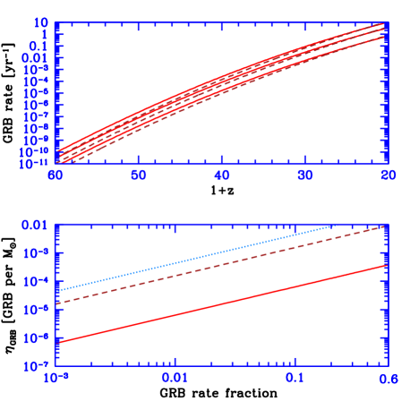
Figure 3: Top panel: Redshift distribution of GRBs for various POP III contribution to the total Swift detection sample. We consider a spectral index of $-1$ (solid curves) and also a spectral index of $-1.6$ (dashed curves). For the first case ($\bar{\alpha}=-1$) we consider a contribution of (top to bottom) $15,5$ and $1$ GRBs per year from redshifts of $20-60$, which results in $\eta_{GRB}=1.1~{}10^{-4}$,$3.5~{}10^{-5}$ and $7.1~{}10^{-6}$ GRBs per solar mass respectively. For the second case ($\alpha=-1.6$) we consider (top to bottom) $15,5$ and $1$ GRBs per year from the relevant redshifts. The resulting upper limit on the efficiency is $\eta_{GRB}=2.6~{}10^{-3},8.7~{}10^{-4}$ and $1.7~{}10^{-4}$ GRBs per solar mass, respectively. Lower panel: $\eta_{GRB}$ for various fractional contribution of GRBs out of $\sim 90$ GRBs per year detected by Swift, from redshifts $20-60$. We consider the spectral index of $-1$ (solid curve) and also spectral index of $-1.6$ (dashed curve). For this latter case we also consider the parameters of model (vi) in Guetta & Piran (2007) (dotted curve), which is less favorable for high luminosity bursts ($b=-2$).

4 DISCUSSION

We have predicted that the redshift of the first observable GRB is most likely $z\sim 60$. This prediction is based on the Naoz, Noter & Barkana (2006) prediction of the redshift of the first observable star.

We have calculated the GRB rate from extremely high redshift ($z=20-60$) POP III stars. We used a simple SFR (based on H₂ cooling) that includes the correct evolution of fluctuations. We assume that at these early times most of the stars formed out of newly accreted gas during mergers. We find that our SFR is consistent with previous analysis at lower redshift (Bromm & Loeb, 2006). However our result predicts a higher rate (see fig. 1) because we consider star formation at higher redshifts.

Using this SFR we evaluated the GRB rate redshift distribution (eq. (4)). We adopted Guetta & Piran (2005) luminosity function, and performed a simple k-correction. We showed that the maximum redshift to which GRBs can be observed depends on their luminosity and on the spectral index (see fig. 2). Using also the $E_{p}$-$L_{iso}$ relation and, as supported by the Schmidt (2001) luminosity hardness correlation, we adopted $\bar{\alpha}=-1$. This value enables high luminosity bursts to be seen to larger distances, i.e., higher redshift.

Using the Swift detection rate we have placed an upper limit on the efficiency of GRB production from POP III stars. For various fractional contribution to the total Swift sample we find different efficiencies (fig. 3). The safest upper limit we set is: $1.1~{}10^{-4}$ GRBs per solar mass. This is a result from a maximal contribution of XRGs to the Swift sample. This sub-sample has $15$ very long ($T_{90}>50$ sec) GRBs per year with no associated redshift and no optical afterglow counterparts (about $\sim 17\%$, of the total Swift detection sample). We also find a more realistic estimate, that the upper limit of GRB efficiency from POP III stars is $3.2~{}10^{-5}$ GRBs per solar mass. This efficiency results in a high redshift GRB contribution of $5\%$ of the Swift sample. Taking the median value $\bar{\alpha}=-1.6$ we find that the upper limit on $\eta_{GRB}$ is $7.8~{}10^{-4}$ GRBs per solar mass.

We caution that we have extrapolated the properties of the observed GRBs to much higher redshift. An additional, important caveat to our model is the strong dependence on the spectral index $\bar{\alpha}$. We point out that given the $E_{p}$-$L_{iso}$ relation it is reasonable to assume that $\bar{\alpha}\lower 2.15277pt\hbox{$\;\buildrel>\over{\sim}\;$}-1.6$. The $E_{p}$-$L_{iso}$ relation is closly related to the Amati et al. (2002) relation. Several authors (e.g., Band & Preece, 2005; Nakar & Piran, 2005) claimed that this relation may be a boundary curve created by the brightest and softest bursts, as a result of observational biases. They suggested that many bursts should be dimmer and harder (though see Amati, 2006). This supports our argument that XRGs should have high $\bar{\alpha}$. For completeness, though, we have shown that if $\bar{\alpha}=-2.2$, Swift can detect only a few GRBs per year from redshift $>20$, and for one GRB per year we find a high upper limit on the efficiency of $4.2~{}10^{-3}$ GRBs per solar mass.

References

- Abel et al. (2002) Abel, T., Bryan, G. L. & Norman, M. L. 2002, Sci, 93.
- Amati et al. (2002) Amati L., et al., 2002, A&A, 390, 81
- Amati (2006) Amati L., 2006, MNRAS, 372, 233
- Band et al. (1993) Band D., et al., 1993, ApJ, 413, 281
- Band & Preece (2005) Band D. L., Preece R. D., 2005, ApJ, 627, 319
- Barkana (2006) Barkana R., 2006, Sci, 313, 931
- Barkana & Loeb (2000) Barkana R., Loeb A., 2000, ApJ, 539, 20
- Barkana & Loeb (2001) Barkana, R., Loeb, A. 2001, PhR, 349, 125
- Barkana & Loeb (2004) Barkana R., Loeb A., 2004, ApJ, 601, 64
- Barkana & Loeb (2006) Barkana R., Loeb A., 2006, astro, arXiv:astro-ph/0611541
- Blain & Natarajan (2000) Blain, A. W., Natarajan, P. 2000, MNRAS, 312, L35
- Bromm, Coppi, & Larson (2002) Bromm V., Coppi P. S., Larson R. B., 2002, ApJ, 564, 23
- Bromm & Loeb (2002) Bromm V., Loeb A., 2002, ApJ, 575, 111
- Bromm & Loeb (2006) Bromm V., Loeb A., 2006, ApJ, 642, 382
- Daigne, Rossi, & Mochkovitch (2006) Daigne F., Rossi E. M., Mochkovitch R., 2006, MNRAS, 372, 1034
- Frail et al. (2001) Frail, D. A., et al., 2001, ApJ, 562, L55
- Fryer, Woosley, & Heger (2001) Fryer C. L., Woosley S. E., Heger A., 2001, ApJ, 550, 372
- Fuller & Couchman, (2000) Fuller, T. M., & Couchman, H. M. P. 2000, ApJ, 544, 6
- Gao et al. (2007) Gao L., Abel T., Frenk C. S., Jenkins A., Springel V., Yoshida N., 2007, astro, arXiv:astro-ph/0610174
- Ghirlanda et al. (2005) Ghirlanda G., Ghisellini G., Firmani C., Celotti A., Bosnjak Z., 2005, MNRAS, 360, L45
- Guetta & Piran (2005) Guetta D., Piran T., 2005, A&A, 435, 421
- Guetta & Piran (2007) Guetta D., Piran T., 2007, astro, arXiv:astro-ph/07011
- Guetta, Piran, & Waxman (2005) Guetta D., Piran T., Waxman E., 2005, ApJ, 619, 412
- Gunn & Peterson (1965) Gunn J. E., Peterson B. A., 1965, ApJ, 142, 1633
- Haiman et al. (1997) Haiman, Z., Rees, M. J. Loeb, 1997, ApJ, 476.
- Heger et al. (2003) Heger A., Fryer C. L., Woosley S. E., Langer N., Hartmann D. H., 2003, ApJ, 591, 288
- Lamb, Donaghy, & Graziani (2005) Lamb D. Q., Donaghy T. Q., Graziani C., 2005, ApJ, 620, 355
- Lamb & Reichart (2000) Lamb D. Q., Reichart D. E., 2000, ApJ, 536, 1
- Mészáros (2002) Mészáros P., 2002, ARA&A, 40, 137
- Nakar (2006) Nakar E., 2006, AAS, 209, #194.04
- Nakar & Piran (2005) Nakar E., Piran T., 2005, MNRAS, 360, L73
- Naoz & Barkana (2005) Naoz S. & Barkana R. MNRAS, 2005, 362, 1047.
- Naoz & Barkana (2007) Naoz S., Barkana R., 2007, MNRAS, in press