Where the Blue Stragglers Roam: Searching for a Link Between Formation and Environment

Abstract

The formation of blue stragglers is still not completely understood, particularly the relationship between formation environment and mechanism. We use a large, homogeneous sample of blue stragglers in the cores of 57 globular clusters to investigate the relationships between blue straggler populations and their environments. We use a consistent definition of “blue straggler” based on position in the color-magnitude diagram, and normalize the population relative to the number of red giant branch stars in the core. We find that the previously determined anti-correlation between blue straggler frequency and total cluster mass is present in the purely core population. We find some weak correlations with central velocity dispersion and with half-mass relaxation time. The blue straggler frequency does not show any trend with any other cluster parameter. Even though collisions may be expected to be a dominant blue straggler formation process in globular cluster cores, we find no correlation between the frequency of blue stragglers and the collision rate in the core. We also investigated the blue straggler luminosity function shape, and found no relationship between any cluster parameter and the distribution of blue stragglers in the color-magnitude diagram. Our results are inconsistent with some recent models of blue straggler formation that include collisional formation mechanisms, and may suggest that almost all observed blue stragglers are formed in binary systems.

1 Introduction

Blue stragglers are stars that are brighter and bluer (hotter) than the main-sequence turn-off. Having seemingly missed their peers’ cue to make the transition to lower temperatures, stars having their same mass have already evolved off the MS and begun their ascent up the giant branch (GB). First discovered by Sandage (1953) in the cluster M3, blue straggler stars (BSSs) are an example of the inability of standard stellar evolution alone to explain all stars, and are used as the prime example of the complex interplay between stellar evolution and stellar dynamics (e.g. Sills et al., 2005). Numerous formation mechanisms have been proposed over the years, but the currently favored mechanisms are thought to depend on cluster dynamics.

There is a consensus that blue stragglers are the products of stellar mergers between two (or more) low mass MS stars, either through direct stellar collisions or the coalescence of a binary system (Leonard, 1989; Livio, 1993; Stryker, 1993; Bailyn, 1995). In order for a binary system to coalesce, Roche lobe overflow must occur, triggering mass transfer from the outer envelope of an evolved donor onto that of its companion. As such, the process is dependent on the donor’s evolutionary state. Collisions, on the other hand, do not depend as much on the evolutionary status of the participants since in this case two (or more) stars pass very close to one another, form a brief and highly eccentric binary system, and then rapidly spiral inwards and merge as tidal forces dissipate the orbital energy.

There is evidence to suggest that both formation mechanisms do occur, though the preferred creation pathway appears dependent on the cluster environment (e.g. Warren et al., 2005; Mapelli et al., 2006). Observations from the Hubble Space Telescope (HST) indicate that BSSs are centrally concentrated in globular clusters (Ferraro et al., 1999), though they have been detected throughout all clusters that have been surveyed well. The BSS populations have been found to have a bimodal radial distribution in clusters like M55 (Zaggia et al., 1997), M3 (Ferraro et al., 1997), and 47 Tuc (NGC 104) (Ferraro et al., 2004), with elevated numbers in the cores followed by a ”zone of avoidance” at a few core radii and a final rise in BS numbers towards the cluster outskirts. This bimodal trend is thought to arise because two separate formation mechanisms are dominating in the core and in the cluster periphery, with mass transfer predominantly taking place in the outer, less dense regions and collisions mainly occurring towards the cluster center. In support of this last point, eclipsing binaries consisting of main sequence components having short periods and sharing a common envelope, called contact or W UMa binaries, have been observed among BSSs in globular (Mateo, 1990; Yan & Mateo, 1994) and open clusters (Ahumada & Lapasset, 1995).

There is an additional complication, however, when considering the effects of stellar collisions. It has been suggested that collisions need not only occur between two single stars in exceptionally dense environments, but rather might also occur in less dense systems via resonant interactions between primordial binaries (Bacon, Sigurdsson & Davies, 1996). Two binary pairs locked in a tightly bound 4-body system can actually increase the rate of collisions by increasing the collisional cross-section of the system (Fregeau et al., 2004). Indeed, multiple collisions are thought to be responsible for some of the blue stragglers we see, in particular those having masses around twice that of our Sun or more (Sepinsky, 2000), or the unusual blue straggler binary system in 47 Tucanae which probably requires 3 progenitor stars (Knigge et al., 2006). Clearly both cluster dynamics and binary star populations will determine how many of these binary-mediated collisions will occur.

Recently, Piotto et al. (2004) examined the CMDs of 56 different GCs, comparing the BSS frequency to cluster properties like total mass (absolute luminosity) and central density. The relative frequencies were approximated by normalizing the number of BSSs to the HB or the red giant branch (RGB), though the results did not depend on which specific frequency they chose. They found that the most massive clusters had the lowest frequency of BSSs, and that there was little or no correlation between BSS frequency and cluster collisional parameter. They also showed that the BSS luminosity function for the most luminous clusters had a brighter peak and extended to brighter luminosities than did that of the fainter clusters.

The absence of a correlation between BSS frequency and collision number, in particular, is surprising, since other evidence suggests that dynamical interactions do affect stellar populations in GCs. For example, GCs host enhanced numbers of unusual short-period binary systems such as low-mass X-ray binaries (LMXBs; (Dieball et al., 2005)), cataclysmic variables (CVs; (Knigge et al., 2003)), and millisecond pulsars (MSPs; (Edmonds et al., 2003)). These objects, like blue stragglers, are thought to trace the dynamically-created populations of clusters. Their presence has been linked to the high densities found in the cores of GCs, which are thought to lead to an increase in the frequency of close encounters and thus in the formation rate of exotic binary systems. Indeed, the number of close binaries in GCs observed in X-rays has been shown to be correlated with the predicted stellar encounter rate of the cluster (Pooley et al., 2003).

A useful quantity for parameterizing the surface brightness distribution of GCs is the core radius, $r_{c}$, defined as the distance from the cluster center at which the surface brightness is half its central value. That is, at a distance of $r_{c}$ from the center of a King model globular cluster, the density is expected to have dropped off to around a third of the density at the cluster center (Spitzer, 1987). This then implies that the core encloses the densest regions of the cluster by at least a factor of a few and hence one would expect interactions between stars, specifically collisional processes, to occur with the greatest frequency therein.

In our quest to determine the cluster environment’s effect on BSS formation, we decided to focus solely on the stars found within the core in order to isolate the ones most likely to undergo stellar encounters. We wanted to search for empirical evidence for collisional BSS formation, and the cores of clusters are the most likely place for collisions to not only occur, but also to dominate (Mapelli et al., 2006; Ferraro et al., 2004). Previous attempts to connect blue straggler populations to global cluster properties (Piotto et al., 2004; Davies et al., 2004) did not attempt to focus on a single, homogeneous environment. By concentrating solely on the core, we therefore maintain consistent sampling from cluster to cluster. We note that while directing our attention to the core allows us to isolate an approximately uniform dynamical environment, it also presents a statistical complication in post-core collapse clusters since these tend to have small core radii and the star counts therein thus tend to be restricted. Fortunately, only a small fraction of the clusters used in this paper have undergone core collapse and so this effect should not have a significant impact on our results.

In this paper, we use Hubble Space Telescope (HST) data to look for possible trends between relative BSS frequency and various cluster parameters, including total cluster mass, central density, central velocity dispersion as well as collisional parameters. We discuss our dataset, as well as our methodology for BSS selection in the cluster CMDs in Section 2. In Section 4 we present our results, including trends in the relative BSS frequencies as well as a comparison of blue straggler luminosity functions (BSLFs). We summarize and discuss our findings in Section 6.

2 The Data

The color-magnitude diagrams and photometric databases for 74 Galactic globular clusters were used in this paper. The observations, taken from Piotto et al. (2002), were made using the HST’s WFPC2 camera in the F439W and F555W bands, with the PC camera centered on the cluster center in each case. Generally, the field of view for each cluster contains anywhere from a few thousand to roughly 47,000 stars. Of the 74 potential GGCs, only 57 were deemed fit for analysis, with the remaining 17 having been discarded due to poor reliability of the data at or above the main sequence turn-off based on the overall appearance of their respective CMDs. The positions of the stars, as well as their magnitudes in both the F439W and F555W bands and the B and V standard Johnson system, can be found at the Padova Globular Cluster Group Web pages at http://dipastro.pd.astro.it/globulars. Core radii and other cluster parameters were taken from (Harris, 1996) and (Pryor & Meylan, 1993).

The data available at the Padova website have not been corrected for completeness. This could be a problem for our analysis if we cannot accurately determine the total number of blue stragglers, red giant, horizontal branch, and extended horizontal branch stars. However, we do not expect this to be an issue in this paper. All the clusters that we retained in our sample have clearly-defined main sequence turn-offs and sub-giant branches. The populations of interest are brighter than the turn-off, by definition, and should be less affected by photometric errors and completeness. We expect that the corrections for the faintest objects that we identify as blue stragglers should be on the order of one star or less, which will not change the results of this paper. To be safe, however, stars having sufficiently large errors in $m_{555}$ and $m_{439}$, respectively denoted by $\sigma_{f555W}$ and $\sigma_{f555W}$, were also rejected from our counts if their total error was more than 0.1 magnitudes.

We defined a set of boundaries in the color-magnitude diagram for each of our populations of interest: blue stragglers, red giant branch stars, horizontal branch stars, and extended horizontal branch stars. The details of these definitions can be found in the appendix. The boundaries of our blue straggler selection box were ultimately chosen for consistency. By eliminating potential selection effects such as “by eye” estimates, we were able to minimize the possibility of counting EHB or MSTO stars as BSSs. Moreover, since we are considering relative frequencies and there is a possibility of mistakenly including stars other than BSSs in our counts, it seems prudent that we at least make the attempt to systematically chose stars in all clusters. We are most interested in using the evolved populations to normalize the number of blue stragglers, both to give a sense of photometric error and to remove the obvious relation that clusters with more stars have more blue stragglers. Therefore, we limited ourselves to red giants with the same luminosities as the blue stragglers. These boundaries are shown for NGC 5904 in Figure 1. The full data for all clusters is given in the appendix.

Figure 1: CMD for the cluster NGC 5904 with RGB, BS, HB, and EHB boundaries overlaid.

3 Methods of Normalization

With our sample of core BS, HB, EHB and RGB stars established consistently from cluster to cluster, it was then necessary to address the issue of normalization. As one might expect, clusters having more stars tend to be home to a larger population of BSSs. Number counts of stars therefore had to be converted into relative frequencies. Previously, this was done by dividing the number of BSSs by either the number of horizontal branch stars (Piotto et al., 2004):

$$F^{HB}_{BSS}=\frac{N_{BSS}}{N_{HB}},$$ (1)

or by the total cluster mass (De Marchi et al., 2006):

$$F^{M_{tot}}_{BSS}=\frac{N_{BSS}}{M_{tot}}$$ (2)

Piotto et al. (2004) also looked at using the number of RGB stars for normalization but after finding similar results, decided to simply use the HB. The preferred means of normalization is a matter of some debate and hence we similarly calculated relative frequencies in a few separate ways in order to gauge which is best. Frequencies were normalized using the HB, the EHB, the HB & the EHB, and the RGB:

$$F^{HB}_{BSS} = \frac{N_{BSS}}{N_{HB}}$$ (3)

$$F^{EHB}_{BSS} = \frac{N_{BSS}}{N_{EHB}}$$ (4)

$$F^{HB+EHB}_{BSS} = \frac{N_{BSS}}{N_{HB}+N_{EHB}}$$ (5)

$$F^{RGB}_{BSS} = \frac{N_{BSS}}{N_{RGB}}$$ (6)

Plotting these frequencies against the total V magnitude, previously shown to exhibit a clear anti-correlation (Piotto et al., 2004), proved that using the RGB gives us the tightest relationship. This reduction of scatter was similarly observed upon comparing the BSS frequency to other cluster parameters like the central surface brightness, the central velocity dispersion, as well as the collisional rate. Figure 2 shows the BSS frequency versus the total absolute V magnitude of the cluster for all four normalization methods.

Figure 2: Plots of the core BSS frequency versus the total cluster V magnitude. Frequencies were normalized using RGB stars (bottom right), HB stars (bottom left), EHB stars (top right), and finally, HB & EHB stars combined (top left).

4 Results

Having obtained the numbers and frequencies of blue stragglers in the cluster cores, we attempted to determine correlations between the blue straggler frequency and global cluster properties such as total mass, velocity dispersion, core density, etc. If the preferred BSS formation mechanism in the core is direct stellar collisions, then we should see a link between clusters with higher instances of collisions and more pronounced BSS populations; if the formation mechanism is not collisions, we would still expect to see a relationship between the properties of the cluster and its stellar populations.

The central surface brightness and the core radius were taken from Harris (1996). Values for the central velocity dispersion were taken from Pryor & Meylan (1993). Any other parameters, including the central density and the total absolute luminosity, came from Piotto et al. (2002), with the exception of the normalized cluster ages which were taken from De Angeli et al. (2005) and for which the Zinn & West (1984) metallicity scale values were employed. Error bars for all plots were calculated assuming Poisson statistics.

It should be noted here that while the number of blue straggler stars in a core is a tracer of the total number of stars in the core, as well as of the total number of HB and RGB stars, we found no correlation between the number of blue stragglers and the number of EHB stars. It has been speculated (Ferraro et al., 2003) that there might be a connection between BSS and EHB populations. The trend in that paper (of 6 clusters) was that clusters either had bright blue stragglers or EHB stars, but not both. With this larger self-consistent sample, we do not find the same result. The number of EHB stars seems to be completely independent of how many bright blue stragglers exist in the cluster.

Relative frequencies appeared independent of the majority of the cluster parameters analyzed, with a couple of noteworthy exceptions. One trend observed was that the least massive clusters (those having the lowest absolute luminosities) had the highest relative frequencies of blue stragglers, and vice versa. This anti-correlation was previously observed by Piotto et al. (2004), though their choice of BSS selection and chosen method of normalization arguably led to a greater degree of scatter in their plots. According to our analysis, using the HB for normalization yielded correlations that were overall not as tight as those made using the RGB. They also did not distinguish between blue stragglers inside or outside of one core radius but simply counted the stars in their observed fields. Given the bimodality of the observed BSS radial distribution in some GCs, this could have resulted in the inclusion of BSSs that were never subject to the same dynamical conditions as those BSSs found in the core.

A similar anti-correlation was found between F_BSS and the central velocity dispersion, shown in Figure 3. This is perhaps unsurprising, since velocity dispersion is known to be correlated with cluster mass (Djorgovski et al., 1994). The blue straggler frequencies showed no clear dependence on any other cluster parameters, including the central density, the central surface brightness, and the cluster age.

Figure 4 shows the blue straggler frequency versus the core and half-mass relaxation times. While weak anti-correlations were found with both the core and half-mass relaxation times, F_BSS was found to show a stronger anti-correlation with the latter. Moreover, it seems as though the distribution begins to flatten out at higher $logt_{h}$, specifically beyond around $10^{9}$ years.

Figure 3: Plots of the core BSS frequency versus the logarithm of the central density (bottom right), the central surface brightness (bottom left), the relative cluster age (top left), and the central velocity dispersion (top right). Frequencies were normalized using RGB stars. The central density is given in units of L_⊙ pc^-3, the central surface brightness in units of V mag arcsecond^-2, and the central velocity dispersion in units of km s^-1. The cluster age is normalized, however, and its values represent the ratio between the cluster age and the mean age of a group of metal-poor clusters as described in De Angeli et al. (2005).

Figure 4: Plots of the core BSS frequency versus the logarithm of the core relaxation time in years (top), and the logarithm of the relaxation time at the half-mass radius in years (bottom). Frequencies were normalized using RGB stars. Note the anti-correlation that exists between F_BSS and log $t_{h}$.

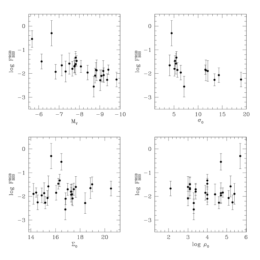
Figure 5: Plots of the brightest core BSS frequency versus the logarithm of the central density (bottom right), the central surface brightness (bottom left), the total cluster V magnitude (top left), and the central velocity dispersion (top right). Frequencies were normalized using RGB stars. The central density is given in units of L_⊙ pc^-3, the central surface brightness in units of V mag arcsecond^-2, the cluster magnitude in V mag, and the central velocity dispersion in units of km s^-1.

We also considered the brightest blue stragglers (BBSSs) separately, under the assumption that these stars are most likely to be collision products. Figure 2 of Monkman et al. (2006) shows that, in the case of 47 Tuc (NGC 104), the number of bright blue stragglers falls off noticeably outside the cluster core. These brightest blue stragglers found only within the core have a B magnitude of less than about 15.60 mag, or a V magnitude of less than about 15.36 mag. Assuming the BBSSs in other clusters are similar to the ones found in 47 Tuc, we defined the brightest BSSs as those having a V magnitude of 1.74 mag brighter than that of the MSTO. As illustrated in Figure 5, the usual trends with $M_{V}$ and the central velocity dispersion were found. No new trends between the BBSS relative frequencies and any cluster parameters emerged.

Figure 5: Plots of the brightest core BSS frequency versus the logarithm of the central density (bottom right), the central surface brightness (bottom left), the total cluster V magnitude (top left), and the central velocity dispersion (top right). Frequencies were normalized using RGB stars. The central density is given in units of L_⊙ pc^-3, the central surface brightness in units of V mag arcsecond^-2, the cluster magnitude in V mag, and the central velocity dispersion in units of km s^-1.

We also looked at the relative BSS frequencies in only the most massive clusters for which $M_{V}<$ -8.8 under the assumption of Davies et al. (2004) that the BSSs in these clusters should predominantly be collision products. Collisional BSSs are thought to be brighter than those formed from primordial binaries. As illustrated in Figure 6, no trends were found between BSS relative frequencies and any cluster parameters when clusters with $M_{V}>$ -8.8 were ignored. Indeed, the previously established trend between $M_{v}$ and F_BSS is considerably weakened by eliminating clusters with $M_{V}>$ -8.8.

Figure 6: Plots of the core BSS frequency in only the brightest clusters ($M_{V}<-8.8$) versus the logarithm of the central density (bottom right), the central surface brightness (bottom left), the total cluster V magnitude (top left), and the central velocity dispersion (top right). Frequencies were normalized using RGB stars. The central density is given in units of L_⊙ pc^-3, the central surface brightness in units of V mag arcsecond^-2, the cluster magnitude in V mag, and the central velocity dispersion in units of km s^-1.

BSS frequencies were also plotted against a parameter used to approximate the rate of stellar collisions per year. Following Pooley & Hut (2006),

$${\Gamma}=\frac{{\rho}_{0}^{2}r_{c}^{3}}{{\sigma}_{0}},$$ (7)

where $\rho_{0}$ is the central density in units of L_⊙ pc^-3, $\sigma_{0}$ is the central velocity dispersion in km s^-1 and $r_{c}$ is the core radius in parsecs. If there is a tight correlation between the fraction of blue stragglers and $\Gamma$, then we can conclude that direct stellar collisions are responsible for most of the blue stragglers in cluster cores. Figure 7 shows, if anything, a decline in BSS frequency with increasing collisional rate. This weak anti-correlation is likely not an artifact of the more populous clusters having more stars available to undergo collisions since we are dealing with normalized BSS frequencies as opposed to pure number counts. This anti-correlation has been seen by Piotto et al. (2004) and Sandquist (2005) for blue straggler populations from a larger region of the cluster. The trend is weak, and one could argue that there is no correlation.

Figure 7: Plot of the BSS frequency within the cluster core versus the rate of stellar collisions per year using Equation 7 as the collisional parameter (top). $\rho_{0}$ is the central density in units of L_⊙ pc^-3, $\sigma_{0}$ is the central velocity dispersion in km s^-1, and $r_{c}$ is the core radius in parsecs. BSS frequency is also plotted against the probability of a stellar collision occurring within the core in one year (bottom). Frequencies were normalized using core RGB stars.

An additional comparison can be made to the probability that a given star will undergo a collision in one year, denoted by $\gamma$. We divide the rate of stellar collisions by the total number of stars in the cluster core, $N_{\rm star}$, found by directly counting them in Piotto et al.’s (2002) database and then multiplying by the appropriate geometrical correction factor. In order for our counts to be representative of the entire core, it was necessary to extrapolate our results in the case of clusters for which only a fraction of the core was sampled. Therefore, the total number of stars was multiplied by the ratio of the entire core area to that of the sampled region in each cluster. Figure 7 clearly shows that there is no dependence of F_BSS on $\gamma$. Similar results were also found when we used the collisional parameter given in Piotto et al. (2004). We also looked for connections between both $\Gamma$ and $\gamma$ and the brightest blue stragglers, and the blue stragglers in the brightest clusters. We found no trend in either case.

To quantify these dependences or lack thereof, we calculated the Spearman correlation coefficients (Press et al., 1992; Wall & Jenkins, 2003) between the blue straggler frequency and a variety of cluster parameters. The results are given in Table 3. The correlation coefficient $r_{s}$ ranges from 0 (no correlation) to 1 (completely correlated), or to -1 (completely anti-correlated). The third column, labeled ‘Probability’, gives the chance that these data are uncorrelated. Clearly the most important anti-correlations are with the total cluster magnitude and the central velocity dispersion (the Spearman coefficient for $M_{V}$ is positive for an anti-correlation because the magnitude scale is backwards). The anti-correlation with half-mass relaxation time also shows up here, and the frequency of blue stragglers in clusters may also be anti-correlated with the core relaxation time and collision rate, although this is not conclusive from these data.

Table 1: Spearman Correlation Coefficients

Parameter	$r_{s}$	Probability
Total cluster V magnitude	0.76	7.2E-12
Central velocity dispersion	-0.70	1.0E-05
Half-mass relaxation time	-0.53	2.5E-05
Core relaxation time	-0.43	1.1E-03
Collision rate	-0.41	0.02
Surface brightness	0.17	0.20
Central density	0.08	0.58
Collision probability	-0.09	0.63
Age	0.02	0.91

5 Blue Straggler Luminosity Functions

Having investigated the relationship between the frequency of blue stragglers and their host cluster properties, we now turn to looking at the details of the blue straggler population itself. Cumulative blue straggler luminosity functions (BSLFs) were made for all 57 clusters in our sample. The magnitude of the MSTO differs from cluster to cluster and so, in order to correct for these discrepancies, it was subtracted from the BSS magnitudes in each cluster.

We wanted to quantify the shape of these luminosity functions in order to determine if there were any connections between BSLF shape and global cluster parameters. We found that all the BSLFs could be well-fit using a quadratic (but not a linear) function of magnitude. Some examples of the fits are given in the top panel of Figure 8. The fits for all clusters are given in the bottom panel.

We looked at each of the quadratic coefficients as a function of all of the cluster parameters, and found that the coefficients had no dependency on any parameter, including total cluster magnitude or metallicity. We were particularly interested in metallicity since the BSLF is a measure of the properties of BSS stellar evolution, which could depend on metallicity. According to these data, it does not.

Figure 8: Cumulative BS luminosity functions. The top panel shows the BSLFs for NGC 104 (47 Tucanae) and NGC 7099 (M30) (solid lines) along with quadratic fits to those functions (dashed lines). The bottom panel shows the quadratic fits to all cluster BSLFs.

Piotto et al. (2004) argued that if the BSS formation mechanisms depend on the cluster mass, then one would expect the blue straggler LFs to likewise depend on the mass. They predicted that the luminosity distribution of collisionally produced BSSs should differ from those created via mass transfer or the merger of a binary system due to different resulting interior chemical profiles. They were able to generate separate BSLFs for clusters with $M_{V}<$ -8.8 and $M_{V}>$ -8.8 in support of their hypothesis. Upon subtracting MSTO magnitudes from peak BSLF magnitudes and creating individual BSLFs for clusters above and below a total V magnitude of -8.8, we found the difference between the two sub-sets of BSLFs to be negligible. Interestingly, there were in total only 11 clusters in our dataset for which $M_{V}<$ -8.8 and so, had we found any potential trends, their reliability would be suspect. Any generalizations made regarding the most massive clusters should be disregarded due to the small number of clusters in the Piotto et al. (2002) dataset in this regime.

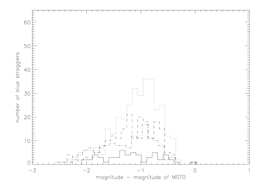
Figure 9: Blue straggler luminosity functions, binned according to total cluster magnitude. The solid line is for clusters with $M_{V}$ between -6 and -7; dotted line for clusters with $M_{V}$ between -7 and -8; dashed line for clusters with $M_{V}$ between -8 and -9, and the dash-dotted line is for clusters with $M_{V}$ between -9 and -10.

We repeated this experiment by binning our BSLFs according to cluster magnitude, in bins of size 1 magnitude. The results are shown in Figure 9. We see no trend in the peak of the BSLF with cluster magnitude. We also tried binning the BSLFs by central density (in bins of size 1 in $\log(\rho)$) and by half-mass relaxation time (in bins of size 0.5 in $\log(t_{h})$). Again, we found no trend in the peak magnitude or shape of the luminosity function for any of these parameters. We expect, given our analysis of the shapes of the cumulative BSLFs, that binning by any other cluster parameter will similarly yield no trends. Just to check, we performed a Kolmogorov-Smirnov test on the luminosity functions that were binned by absolute cluster magnitude (those shown in Figure 9). No pairs of distributions were drawn from the same parent distribution with more than a few percent probability. The closest pair ($-7<M_{V}<-6$ and $-9<M_{V}<-8$) have a 57% probability of being drawn from the same distribution; and all other pairs were below the 10% level.

Figure 9: Blue straggler luminosity functions, binned according to total cluster magnitude. The solid line is for clusters with $M_{V}$ between -6 and -7; dotted line for clusters with $M_{V}$ between -7 and -8; dashed line for clusters with $M_{V}$ between -8 and -9, and the dash-dotted line is for clusters with $M_{V}$ between -9 and -10.

6 Summary & Discussion

We used the large homogeneous database of HST globular cluster photometry from Piotto et al. (2004) to investigate correlations of blue stragglers with their host cluster properties. First, we applied a consistent definition of “blue straggler” to all our clusters. We chose the MSTO as our starting point and defined our boundaries based only on its location in the CMD. We also defined the location of horizontal branch and extended horizontal branch stars in the CMD. We looked at a variety of normalizations for our BSS frequencies before determining that using the RGB yielded the plots with the least scatter.

There are disappointingly few strong correlations between the frequency of blue stragglers in the cores of these clusters and any global cluster parameter. We confirm the anti-correlation between the the total integrated cluster luminosity and relative BSS frequency found by Piotto et al. (2004); we suggest an anti-correlation with central velocity dispersion based on a high correlation coefficient comparable to that found for the cluster luminosity. At a lower significance are possible anti-correlations with half-mass and core relaxation times.

The relaxation time for a cluster is a measure of how long a system can live before individual stellar encounters become important and the approximation of objects moving in a smooth mean potential breaks down. Globular clusters are the quintessential collisional dynamical systems, since their ages are typically much longer than their relaxation times. It seems sensible that the fraction of blue stragglers, a dynamically created population, should depend on the relaxation times of clusters. The puzzle comes, as usual, in the details. First, we are looking at core blue stragglers, so we might expect the blue straggler fraction to go up with decreasing core relaxation time. The observations do give us this kind of trend, but not a very strong one. We might also expect the blue straggler fraction to depend on the half-mass relaxation time, which is a better measure of the dynamical state of the whole system. The blue straggler fraction does depend on $t_{h}$ in the way that we expect, but only apparently for systems with short dynamical times. Is blue straggler formation a dynamical process which takes a while to turn on? It seems that might be the case.

If the observed anti-correlation between F_BSS and the central velocity dispersion is real, then it follows that random relative motions somehow impede stellar mergers. A similar conclusion can be drawn from the plots of F_BSS versus $\Gamma$ in the event that the speculated anti-correlations are truly representative of the cluster dynamics. Collisional processes therefore seem to somehow interfere with the production of BSSs. If the majority of BSSs are, in fact, the remnants of coalescing binaries then it stands to reason that an increase in the number of close encounters or collisions with other stars could result in the disruption of a larger number of binary systems. On the other hand, if the majority of BSSs are the products of stellar collisions, then it is conceivable that those clusters having the highest collisional frequencies are the most likely to undergo three- or four-body encounters. As such, clusters having the highest collisional rates could also have, on average, the most massive BSSs resulting from an increased incidence of multi-body mergers. This might then contribute to the observed weak anti-correlation between F_BSS and the collisional rate since clusters having a higher incidence of collisions should consequently have a higher incidence of multi-body mergers, resulting in a potentially lower relative BSS frequency. We need more, and more accurate, individual surface gravity measurements of blue stragglers in order to explore the idea that a surplus of more massive BSSs can be found in those clusters with a higher $\Gamma$.

F_BSS was found to be nearly uniform with every other cluster parameter, suggesting that all globular clusters of all properties produce the same fraction of blue stragglers. The lack of a dependence of F_BSS on cluster age implies that whatever the preferred mechanism(s) of BSS formation, it occurs in globular clusters of every age with comparable frequencies. It should be noted that this result does not extend to open clusters. There is a clear correlation of blue straggler frequency with cluster age for open clusters between the ages of 10⁸ and 10¹⁰ years (De Marchi et al., 2006).

Cumulative BSS luminosity functions were analyzed for all 57 GCs. Unlike Piotto et al. (2004), we found no real difference between the BSLFs of the most massive clusters and those of the least massive clusters. In fact, we found no correlation between the shape of the cumulative luminosity function and any other cluster property. These results do not support the notion that differing interior chemical profiles cause collisionally-produced BSSs to have differing luminosities from those created via mass transfer or the coalescence of primordial binaries. It does, however, suggest that either the products of both formation mechanisms cannot be distinguished by their luminosity functions alone, or a single formation mechanism is operating predominantly in all environments.

Trends were also looked for in the brightest blue stragglers, since we suspected their enhanced brightnesses to imply a collisional origin. We also looked at the entire core blue straggler population in the most massive clusters (also thought to be predominantly a collisional population). No trends were observed. Therefore, even putatively collisional blue stragglers show no connection to their cluster environment.

What conclusions can we draw from this near-complete lack of connection between blue stragglers and their environment? We approached this project with the idea of looking only at blue stragglers formed through stellar collisions (those in the core, or the brightest blue stragglers in the core). Having found no correlations, we are forced to acknowledge that our prediction that core blue stragglers are predominantly formed through collisions may be incorrect. This is in disagreement with many arguments in the literature. Those arguments range from discussions of probable encounter rates (Hills & Day, 1976) to the detailed dynamical simulations of Mapelli et al. (2006). It should be noted that while collisions are not solely responsible for their production, they may still play an important role in BSS formation. Indeed, the fraction of close binaries has been found to be correlated with the rate of stellar encounters in GCs (Pooley et al., 2003). It is becoming increasingly clear that GCs represent complex stellar populations and that detailed models are required in order to accurately track their evolution.

It has also become clear, however, that blue stragglers are an elusive bunch. It appears more and more obvious that there are numerous factors working together to produce the populations that we observe. Even if we limit ourselves to consider only those blue stragglers created through binary mergers, we still need to include the effects of cluster dynamics since the binary populations of clusters will be modified through encounters (e.g. Ivanova et al., 2005). Contrary to what Davies et al. (2004) suggest, we do not feel we can reliably say that the effects of collisions will be to explicitly reduce the binary population in the core. Rather, it is likely that the distribution of periods, separations, and mass ratios will be modified through encounters but precisely how remains difficult to predict. Indeed, dynamical processes act to reduce the periods in short-period binaries rather than destroy them, with the binaries at the lower end of the period distribution shifting to even shorter periods the fastest (Andronov et al., 2006). At the same time, wider binaries can be destroyed in clusters as a result of stellar interactions. Therefore, models of blue straggler populations need to be reasonably complex. In this paper, we present observational constraints on those models. Blue straggler populations must be approximately constant for clusters of all ages, densities, concentrations, velocity dispersions, etc.; the number of blue stragglers decreases with increasing cluster mass; and the type, or luminosity function, of blue stragglers is apparently completely random from cluster to cluster. That the luminosity function data appears random perhaps should not have been a surprise. The current blue straggler luminosity function is a convolution of the blue straggler mass function and the blue straggler lifetimes.

There is one important cluster property for which we could not perform this analysis – the cluster binary fraction. If those clusters with a high binary fraction also have higher relative BSS frequencies then this might suggest a preferential tendency towards BSSs forming via coalescence. More importantly, such a trend could be indicative of more massive clusters having a higher frequency of binaries of the right type. That is, more massive clusters may be more likely to harbor binary systems with components in the right mass range and with the right separation to form blue stragglers in the lifetime of the cluster. It therefore seems wise to develop our knowledge of the types of binary systems commonly found in GCs, specifically the mass ratios, periods, and separations thereof. Preston & Sneden (2000) suggest that GCs either destroy the primordial binaries that spawn long-period BS binaries like those observed in the Galactic field, or they were never home to them in the first place. This statement supports the notion that the majority of BSSs formed in globular clusters are the products of the mergers of close binaries, a claim that is not in disagreement with the results of this paper. Work is required on both the observational and theoretical fronts in order to completely understand this ubiquitous, and frustrating, stellar population.

Appendix A Stellar Population Selection Criteria

Color-magnitude diagrams are often so cluttered that distinguishing the blue stragglers from ordinary MSTO stars, or even those belonging to the horizontal and extended horizontal branches, can be a challenging and ambiguous task. In looking at the BSS populations of 6 different GCs, Ferraro et al. (1997) defined boundaries to separate the BSSs from regular MS stars. Using the MSTO as a point of reference, they shifted the CMD of each cluster to coincide with that of M3 for consistency and then divided the blue straggler population into two separate subsamples: bright BSSs with m₂₅₅ $<$ 19 mag and faint BSSs with 19.0 mag $<$ m₂₅₅ $<$ 19.4 mag.

Similarly, De Marchi et al. (2006) studied 216 open clusters (OCs) containing a total of 2105 BSS candidates in order to compare the blue straggler frequency to the cluster mass (total magnitude) and age. They found an anti-correlation between BSS frequency and total magnitude, extending the results of Piotto et al. (2004) to the open cluster regime. They also found a good correlation between the BSS frequency and the cluster age, suggesting that at least one of the BSS formation mechanisms requires a much longer time-scale to operate in order to make its mark on a stellar population. De Marchi et al. defined their own criteria for the selection of blue stragglers and, contrary to Ferraro et al. (1997), defined boundaries by shifting the zero-age main sequence (ZAMS) towards brighter V magnitudes and enclosed the resident BSSs with borders above and below.

We chose to take as our starting point the sharpest point in the bend of the MSTO centered on the mass of points that populate it (denoted by $((B-V)_{0},V_{0})$) . From here, we defined a “MSTO width”, $w$, in the $m_{439}-m_{555}$ plane to describe its approximate thickness, and then established a second reference point, $(B-V,V)$, by shifting $w/4$ mag lower in $m_{439}-m_{555}$ and $5w/8$ lower in $m_{555}$, as indicated in Equation A1:

$$B-V = (B-V)_{0}-w/4$$ (A1)

$$V = V_{0}-5w/8$$ (A2)

This shift ensured that our boundary selection starting point, namely the outer edge of the MSTO, was nearly identical for every cluster. In order to separate the BSSs from the rest of the stars that populate the region just above the MSTO, we drew two lines of slope -3.5 in the $(m_{439}-m_{555},m_{555})$-plane made to intersect points shifted from $(B-V,V)$. One line was shifted 0.5 mag lower in $m_{439}-m_{555}$ and 0.1 mag lower in $m_{555}$ from $(B-V,V)$, whereas the other was shifted 2.0 mag lower in $m_{439}-m_{555}$ and 0.4 mag lower in $m_{555}$. These new points of intersection are shown in Equation A3 below:

$$(B-V)_{r} = (B-V)-0.5$$ (A3)

$$V_{r} = V-0.1$$ (A4)

$$(B-V)_{l} = (B-V)-2.0$$ (A5)

$$V_{l} = V-0.4$$ (A6)

Two further boundary conditions were defined by fitting two lines of slope 5.0, chosen to be more or less parallel to the fitted ZAMS, one intersecting a point shifted 0.2 mag higher in $m_{439}-m_{555}$ and 0.5 mag lower in $m_{555}$ from $(B-V,V)$ (top), and another passing through a point 0.2 mag lower in $m_{439}-m_{555}$ and 0.5 mag higher in $m_{555}$ (bottom). These new intersection points are given by:

$$(B-V)_{t,b} = (B-V)\pm 0.2$$ (A7)

$$V_{t,b} = V\mp 0.5$$ (A8)

These cuts eliminate obvious outliers and further distinguish BSSs from HB and EHB stars. The methodology used in De Marchi et al. (2006) for isolating BSSs similarly incorporated the ZAMS, though their upper and lower boundaries were ultimately defined differently, as outlined in Section 1. Finally, one last cut was made to distinguish BSSs from the EHB, namely a vertical one made 0.4 mag lower in $m_{439}-m_{555}$ than the MSTO.

A similar methodology was used to isolate the RGB stars in the cluster CMDs. We are restricting ourselves to RGB stars in the same magnitude range as the blue straggler stars. First, two lines of slope -19.0 in the $(m_{439}-m_{555},m_{555})$-plane were drawn to intersect the MSTO. In order to place them on either side of the RGB, both lines were shifted 0.6 mag lower in $m_{555}$ though it was necessary to apply different color shifts. The left-most boundary was placed 0.15 mag higher in $m_{439}-m_{555}$ while the right-most boundary was placed 0.45 mag higher in $m_{439}-m_{555}$. To fully define our RGB sample, a lower boundary was defined using a horizontal cut made 0.6 mag above the MSTO (lower in $m_{555}$). The upper boundary, on the other hand, was simply defined to be the lower boundary of the HB. RGB stars must therefore simultaneously satisfy:

$$-19.0(B-V)_{RGB}+{(V-0.6)+19.0((B-V)+0.15)}<V_{RGB}$$ (A9)

$$V_{RGB}<-19.0(B-V)_{RGB}+{(V-0.6)+19.0((B-V)+0.45)}$$ (A10)

$$V-0.6<V_{RGB}$$ (A11)

$$V_{RGB}>h+0.4$$ (A12)

Pulling out HB and EHB stars from the cluster CMDs was found to be more difficult than for BSSs and RGB stars due to the awkward shape of the bend as the HB extends down to lower luminosities. Exactly where the HB ends and the EHB begins has always been a matter of some controversy, and so the choice of where to place the boundary was arbitrary but was at least consistent from cluster to cluster.

A vertical boundary was placed 0.5 mag lower in $m_{439}-m_{555}$ than the MSTO to distinguish the end of the HB from the start of the EHB. The center-most part (in absolute magnitude) of the grouping of stars that make up the HB, denoted by $h$, was carefully chosen by eye, and two horizontal borders were subsequently defined 0.4 mag above and below. One more boundary, this time a vertical cut to help distinguish the HB from the RGB, was set 0.3, 0.4, or 0.5 mag higher in $m_{439}-m_{555}$ than the MSTO. The decision of which of these three $HB_{shift}$’s to use was decided for each cluster based on their individual CMDs. Every star in the CMD that fell to the left of this vertical boundary and in between the horizontal ones was taken to be an HB star, and every star that wasn’t already counted as a BSS or a member of the HB was then taken to be an EHB star. Thus, HB stars, denoted by $((B-V)_{HB},V_{HB})$, must simultaneously satisfy:

$$(B-V)_{HB}<(B-V)+HB_{shift}$$ (A13)

$$h-0.4<V_{HB}<h+0.4$$ (A14)

Finally, it was necessary to eliminate any very faint EHB stars to avoid including any white dwarfs in our sample. Hence, a final boundary was set 3.5 mag below the lower boundary of the HB. This then implies that EHB stars, denoted by $((B-V)_{EHB},V_{EHB})$, must satisfy:

$$(B-V)_{EHB}<(B-V)-0.5$$ (A15)

$$h+0.4<V_{EHB}<h+0.4+3.5$$ (A16)

One small region of concern for the EHB remains undefined in the CMDs, namely the portion just above the “left” BSS boundary with slope -3.5 that also falls to the right of our vertical EHB/BSS dividing line and below the lower HB boundary. For simplicity, we treat these stars as belonging to the EHB, though note that our frequencies would not have been altered by much had we taken them to be BSSs, and even less so had we taken them to be HB stars. As such, in addition to the above criteria, EHB stars can also simultaneously satisfy:

$$(B-V)_{EHB}>(B-V)-0.5$$ (A17)

$$V_{EHB}>h+0.4$$ (A18)

$$V_{EHB}<-3.5(B-V)_{EHB}+{(V-2.0)+3.5((B-V)-0.4)}$$ (A19)

In Table 4, we give the cluster name, the number of BSS, HB, EHB, RGB, and core stars, as well as parameters needed to make these selections: the width of the main sequence $w$, the position of the MSTO, and the level of the horizontal branch.

Table 2: Population Selection Criteria and Numbers

Cluster	NBSS	NHB	NEHB	NRGB	Ncore	$w$	(B-V)MSTO	VMSTO	Vhb
NGC0104	35	200	2	648	28924	0.150	0.510	17.100	13.800
NGC0362	41	118	14	343	20359	0.140	0.390	18.300	15.200
NGC1261	6	21	1	51	9265	0.220	0.410	19.600	16.700
NGC1851	13	43	5	117	21923	0.200	0.480	18.900	16.000
NGC1904	25	23	54	238	14485	0.200	0.450	19.500	16.000
NGC2808	47	212	132	975	46328	0.250	0.400	18.700	15.500
NGC3201	14	20	2	83	3175	0.200	0.530	17.100	14.100
NGC4147	16	14	7	53	2675	0.180	0.400	20.000	16.900
NGC4372	11	11	7	95	1847	0.170	0.430	17.700	14.500
NGC4590	24	30	2	180	5253	0.150	0.380	18.800	15.500
NGC4833	20	50	51	300	6461	0.180	0.400	17.800	14.500
NGC5024	28	69	85	421	12997	0.250	0.370	20.000	16.700
NGC5634	27	54	44	252	6868	0.300	0.350	20.800	17.500
NGC5694	17	5	133	184	14914	0.290	0.460	21.300	17.800
NGC4499	23	46	1	186	3221	0.250	0.390	20.100	16.900
NGC5824	34	52	139	233	28046	0.310	0.400	21.100	18.000
NGC5904	16	69	38	270	14696	0.190	0.410	18.100	15.000
NGC5927	33	117	1	324	15856	0.300	0.630	18.700	15.200
NGC5946	1	7	49	89	7032	0.310	0.520	19.000	15.500
NGC5986	21	68	150	588	16141	0.210	0.430	18.900	15.600
NGC6093	27	22	132	356	11390	0.300	0.520	18.800	15.400
NGC6171	14	24	3	93	2972	0.220	0.670	17.900	14.600
NGC6205	14	25	168	735	13276	0.300	0.430	18.300	14.700
NGC6229	38	86	79	385	8999	0.330	0.450	21.100	18.000
NGC6218	26	5	34	166	5142	0.170	0.480	17.500	13.900
NGC6235	7	3	22	106	3288	0.230	0.420	19.100	15.500
NGC6266	24	76	80	483	21369	0.300	0.510	17.900	14.700
NGC6273	32	21	178	715	32692	0.310	0.490	18.300	15.000
NGC6284	4	11	28	74	7890	0.220	0.500	19.600	16.400
NGC6287	14	25	26	132	4827	0.300	0.520	18.700	15.400
NGC6293	5	5	24	52	16707	0.180	0.370	18.400	15.200
NGC6304	15	51	2	162	11524	0.230	0.580	18.000	14.600
NGC6342	7	8	0	34	4809	0.310	0.590	18.800	15.400
NGC6356	23	187	2	565	18223	0.320	0.580	20.000	16.500
NGC6362	23	37	2	161	4084	0.160	0.510	18.500	14.900
NGC6388	64	479	54	1054	46933	0.500	0.590	19.100	15.700
NGC6402	19	181	145	445	12347	0.380	0.510	18.700	15.400
NGC6397	4	0	4	3	16507	0.100	0.370	15.700	12.500
NGC6522	0	3	5	28	16426	0.210	0.490	18.600	15.100
NGC6544	3	0	2	8	3196	0.230	0.530	16.300	12.700
NGC6584	22	51	3	291	5679	0.220	0.400	19.500	16.100
NGC6624	15	25	0	104	12537	0.300	0.580	18.600	15.200
NGC6638	18	51	5	238	6737	0.250	0.530	18.900	15.500
NGC6637	20	82	1	294	8523	0.260	0.570	18.800	15.400
NGC6642	14	26	1	56	2938	0.200	0.510	18.600	15.200
NGC6652	14	16	4	64	5749	0.150	0.560	19.000	15.600
NGC6681	4	2	4	24	6056	0.170	0.450	18.800	15.400
NGC6712	39	64	3	294	9540	0.250	0.500	18.100	14.800
NGC6717	10	3	1	17	1623	0.220	0.470	18.500	15.400
NGC6723	14	72	25	290	7052	0.180	0.510	18.600	15.300
NGC6838	17	9	3	56	2132	0.150	0.570	17.000	13.800
NGC6864	27	165	14	391	10132	0.230	0.440	20.200	17.200
NGC6934	18	56	11	201	9472	0.190	0.430	19.700	16.600
NGC6981	18	50	1	149	5704	0.170	0.390	19.800	16.800
NGC7078	10	47	32	223	32581	0.210	0.380	18.600	15.500
NGC7089	5	28	69	244	11723	0.190	0.390	19.000	15.500
NGC7099	10	8	56	30	8010	0.200	0.380	18.300	15.000

Appendix B Erratum: “Where the Blue Stragglers Roam: Searching for a Link Between Formation and Environment” (ApJ, 661, 210 [2007]); published May 1, 2008

The paper ‘Where the Blue Stragglers Roam: Searching for a Link Between Formation and Environment’ was published in ApJ, 661, 210 (2007). We made an error in our conversion of arcseconds to pixels when calculating the core radii for the WF chips. Using a conversion factor of 0.046 arcseconds/pixel led to an over-estimation of the size of the core in pixels by a factor slightly exceeding 2. Below, we provide a corrected version for each figure shown in our original paper, in addition to corrected versions of both tables. The overall trends are unaffected and our figures remain similar, apart from a scale change in Figure 7 which is a result of the error made in the calculation of our core radii. The new Spearman correlation coefficients also remain similar.

We also take this opportunity to note that the accuracy of Piotto et al.’s (2002) assumption that each cluster core has been centered on the PC chip proved to be more of a concern when considering these smaller radii since for clusters with small $r_{c}$, the core could be offset from the center of the PC chip by more than one core radius. For this erratum, we calculated our own cluster centers by binning the stellar positions on the PC chip, fitting Gaussians to the corresponding histograms in both the x and y directions, and then using the peak of the distributions to extract the cluster centers (available upon request). The pixel coordinates are given such that the lower left corner of the WF3 chip is at (x,y) = (0,0). The center of the PC chip is then at (984,984), in units of WF chip pixels.

We present the corrected counts of blue stragglers and other populations in Table 2, and present our revised figures in this erratum. The results from our previous paper remain essentially unchanged.

Figure 2: Plots of the core BSS frequency versus the total cluster V magnitude. Frequencies were normalized using RGB stars (bottom right), HB stars (bottom left), EHB stars (top right), and finally, HB & EHB stars combined (top left).

Figure 3: Plots of the core BSS frequency versus the logarithm of the central density (bottom right), the central surface brightness (bottom left), the relative cluster age (top left), and the central velocity dispersion (top right). Frequencies were normalized using RGB stars. The central density is given in units of L_⊙ pc^-3, the central surface brightness in units of V mag arcsecond^-2, and the central velocity dispersion in units of km s^-1. The cluster age is normalized, however, and its values represent the ratio between the cluster age and the mean age of a group of metal-poor clusters as described in De Angeli et al. (2005).

Figure 4: Plots of the core BSS frequency versus the logarithm of the core relaxation time in years (top), and the logarithm of the relaxation time at the half-mass radius in years (bottom). Frequencies were normalized using RGB stars. Note the anti-correlation that exists between F_BSS and log $t_{h}$.

Figure 6: Plots of the core BSS frequency in only the brightest clusters ($M_{V}<-8.8$) versus the logarithm of the central density (bottom right), the central surface brightness (bottom left), the total cluster V magnitude (top left), and the central velocity dispersion (top right). Frequencies were normalized using RGB stars. The central density is given in units of L_⊙ pc^-3, the central surface brightness in units of V mag arcsecond^-2, the cluster magnitude in V mag, and the central velocity dispersion in units of km s^-1.

Figure 7: Plot of the BSS frequency within the cluster core versus the rate of stellar collisions per year using ${\Gamma}=\frac{{\rho}_{0}^{2}r_{c}^{3}}{{\sigma}_{0}}$ as the collisional parameter (top). $\rho_{0}$ is the central density in units of L_⊙ pc^-3, $\sigma_{0}$ is the central velocity dispersion in km s^-1, and $r_{c}$ is the core radius in parsecs. BSS frequency is also plotted against the probability of a stellar collision occurring within the core in one year (bottom). Frequencies were normalized using core RGB stars.

Table 3: Spearman Correlation Coefficients

Parameter	$r_{s}$	Probability
Total cluster V magnitude	0.60	1.95E-06
Central velocity dispersion	-0.56	1.3E-03
Half-mass relaxation time	-0.41	2.1E-03
Core relaxation time	-0.37	6.1E-03
Collision rate	-0.52	3.2E-03
Surface brightness	0.09	0.54
Central density	0.03	0.85
Collision probability	-0.25	0.18
Age	0.04	0.80

Figure 8: Cumulative BS luminosity functions. The top panel shows the BSLFs for NGC 104 (47 Tucanae) and NGC 7099 (M30) (solid lines) along with quadratic fits to those functions (dashed lines). The bottom panel shows the quadratic fits to all cluster BSLFs.

Table 4: Population Selection Criteria and Numbers

Cluster	NBSS	NHB	NEHB	NRGB	Ncore	$w$	(B-V)MSTO	VMSTO	Vhb
NGC0104	26	111	1	344	7398	0.150	0.510	17.100	13.800
NGC0362	29	62	8	181	3541	0.140	0.390	18.300	15.200
NGC1261	8	18	1	40	3241	0.220	0.410	19.600	16.700
NGC1851	9	17	3	53	539	0.200	0.480	18.900	16.000
NGC1904	14	9	22	117	2050	0.200	0.450	19.500	16.000
NGC2808	35	106	76	552	9525	0.250	0.400	18.700	15.500
NGC3201	13	15	2	72	2671	0.200	0.530	17.100	14.100
NGC4147	10	4	4	16	344	0.180	0.400	20.000	16.900
NGC4372	11	11	7	93	1794	0.170	0.430	17.700	14.500
NGC4590	13	13	2	107	2259	0.150	0.380	18.800	15.500
NGC4833	13	35	28	198	3891	0.180	0.400	17.800	14.500
NGC5024	23	39	84	244	3159	0.250	0.370	20.000	16.700
NGC5634	19	30	43	150	1588	0.300	0.350	20.800	17.500
NGC5694	12	2	111	64	544	0.290	0.460	21.300	17.800
IC 4499	15	27	1	112	1755	0.250	0.390	20.100	16.900
NGC5824	16	19	118	73	379	0.310	0.400	21.100	18.000
NGC5904	15	39	19	141	3170	0.190	0.410	18.100	15.000
NGC5927	16	64	0	145	3168	0.300	0.630	18.700	15.200
NGC5946	1	2	39	35	391	0.310	0.520	19.000	15.500
NGC5986	12	40	84	348	6960	0.210	0.430	18.900	15.600
NGC6093	15	12	82	156	1326	0.300	0.520	18.800	15.400
NGC6171	11	10	1	45	837	0.220	0.670	17.900	14.600
NGC6205	7	15	99	354	4285	0.300	0.430	18.300	14.700
NGC6229	26	33	31	151	1484	0.330	0.450	21.100	18.000
NGC6218	14	1	13	68	1715	0.170	0.480	17.500	13.900
NGC6235	4	2	15	62	928	0.230	0.420	19.100	15.500
NGC6266	15	36	43	233	2760	0.300	0.510	17.900	14.700
NGC6273	17	10	104	376	8015	0.310	0.490	18.300	15.000
NGC6284	0	4	9	21	357	0.220	0.500	19.600	16.400
NGC6287	7	17	21	90	916	0.300	0.520	18.700	15.400
NGC6293	3	1	20	25	331	0.180	0.370	18.400	15.200
NGC6304	12	23	2	82	1635	0.230	0.580	18.000	14.600
NGC6342	4	3	0	17	175	0.310	0.590	18.800	15.400
NGC6356	16	112	2	302	3817	0.320	0.580	20.000	16.500
NGC6362	20	28	2	125	3104	0.160	0.510	18.500	14.900
NGC6388	33	174	16	356	2593	0.500	0.590	19.100	15.700
NGC6402	14	98	82	191	6513	0.380	0.510	18.700	15.400
NGC6397	2	0	3	2	96	0.100	0.370	15.700	12.500
NGC6522	4	2	10	33	295	0.210	0.490	18.600	15.100
NGC6544	2	0	2	4	34	0.230	0.530	16.300	12.700
NGC6584	15	28	2	176	2385	0.220	0.400	19.500	16.100
NGC6624	9	9	0	38	454	0.300	0.580	18.600	15.200
NGC6638	15	28	4	169	1915	0.250	0.530	18.900	15.500
NGC6637	18	54	1	179	2681	0.260	0.570	18.800	15.400
NGC6642	7	6	1	33	301	0.200	0.510	18.600	15.200
NGC6652	11	7	4	29	466	0.150	0.560	19.000	15.600
NGC6681	2	0	3	11	92	0.170	0.450	18.800	15.400
NGC6712	31	46	2	164	5197	0.250	0.500	18.100	14.800
NGC6717	5	2	1	7	97	0.220	0.470	18.500	15.400
NGC6723	10	41	19	187	4246	0.180	0.510	18.600	15.300
NGC6838	7	4	2	22	601	0.150	0.570	17.000	13.800
NGC6864	16	84	9	144	1364	0.230	0.440	20.200	17.200
NGC6934	17	42	8	126	2506	0.190	0.430	19.700	16.600
NGC6981	11	34	1	88	2085	0.170	0.390	19.800	16.800
NGC7078	5	16	18	78	777	0.210	0.380	18.600	15.500
NGC7089	5	12	48	136	1989	0.190	0.390	19.000	15.500
NGC7099	9	4	58	17	315	0.200	0.380	18.300	15.000

References

- Ahumada & Lapasset (1995) Ahumada, J. & Lapasset, E. 1995, A&AS, 109, 375
- Andronov et al. (2006) Andronov, N., Pinsonneault, M. H. & Terndrup, D. M. 2006, ApJ, 646, 1160
- Bacon, Sigurdsson & Davies (1996) Bacon, D., Sigurdsson, S. & Davies, M. B. 1996, MNRAS, 281, 830
- Bailyn (1995) Bailyn, C. D. 1995, ARA&A, 33, 133
- Binney & Merrifield (1998) Binney, J. & Merrifield, M. 1998, Galactic Astronomy (Princeton: Princeton University Press)
- Davies et al. (2004) Davies, M. B., Piotto, G., & De Angeli, F. 2004, MNRAS, 348, 129
- De Angeli et al. (2005) De Angeli, F., et al. 2005 AJ, 130, 116
- De Marchi et al. (2006) De Marchi, F. et al. 2006, A&A, astro-ph/0608464
- Dieball et al. (2005) Dieball, A., C., Knigge, C., Zurek, D. R., Shara, M., M., Long, K. S., Charles, P. A., Hannikainen, D. C., & van Zyl, L. 2005, ApJ, 634, L105
- Djorgovski et al. (1994) Djorgovski, S., & Meylan, G. 1994, ApJ, 108, 1292
- Edmonds et al. (2003) Edmonds, P., D., Gilliland, R. L., Heinke, C. O., & Grindlay, J. E. 2003, ApJ, 596, 1177
- Ferraro et al. (1997) Ferraro, F. R. et al. 1997, A&A, 324, 915
- Ferraro et al. (1999) Ferraro, F. R. et al. 1999, ApJ, 522, 923
- Ferraro et al. (2003) Ferraro, F. R., Sills, A., Rood, R. T., Paltrinieri, B., & Buonanno, R. 2003, ApJ, 588, 464
- Ferraro et al. (2004) Ferraro, F. R., Beccari, G., Rood, R. T., Bellazzini, M., Sills, A., & Sabbi, E. 2004, ApJ, 603, 127
- Fregeau et al. (2004) Fregeau, J. M. et al. 2004, MNRAS, 352, 1
- Harris (1996) Harris, W. E. 1996, AJ, 112, 1487
- Hills & Day (1976) Hills, J. G., & Day, C. A. 1976, Astrophys. Lett., 17, 87
- Ivanova et al. (2005) Ivanova, N., Belczynski, K., Fregeau, J. M., & Rasio, F. A. 2005, MNRAS, 358, 572
- Knigge et al. (2003) Knigge, C., Zurek, D. R., Shara, M., M., Long, K. S., & Gilliland, R. L. 2003, ApJ, 599, 1320
- Knigge et al. (2006) Knigge, C., Gilliland, R. L., Dieball, A., Zurek, D. R., Shara, M. M., & Long, K. S. 2006, ApJ, 641, 281
- Leonard (1989) Leonard, P. J. T. 1989, AJ, 98, 217
- Livio (1993) Livio, M. 1993, in ASP Conf. Series 53, Blue Stragglers ed. R. A. Saffer (San Francisco: ASP), 3
- Mapelli et al. (2006) Mapelli, M., Sigurdsson, S., Ferraro, F. R., Colpi, M., Possenti, A. & Lanzoni, B. 2006, MNRAS, astro-ph/0609220
- Mateo (1990) Mateo, M. et al. 1990, AJ, 100, 469
- Monkman et al. (2006) Monkman, E., Sills, A., Howell, J., Guhathakurta, P., de Angeli, F. & Beccari, G. 2006, ApJ, astro-ph/0607053
- Piotto et al. (2002) Piotto, G., et al. 2002, A&A, 391, 945
- Piotto et al. (2004) Piotto, G., et al. 2004, ApJ, 604, L109
- Pooley et al. (2003) Pooley, D., et al. 2006, ApJ, 591, L131
- Pooley & Hut (2006) Pooley, D. & Hut, P. 2006, ApJ, 646, 143
- Press et al. (1992) Press, W. H., Teukolsky, S. A., Vetterling, W. T., & Flannery, B. P. 1992, Cambridge: University Press, —c1992, 2nd ed.
- Preston & Sneden (2000) Preston, G., W. & Sneden, C. 2000, AJ, 120, 1014
- Pryor & Meylan (1993) Pryor C. & Meylan, G. 1993, in ASP Conf. Series 50, Structure and Dynamics of Globular Clusters ed. S. G. Djorgovski & G. Meylan (San Francisco: ASP), 357
- Sandage (1953) Sandage, A. R. 1953, AJ, 58, 61
- Sandquist (2005) Sandquist, E. L. 2005, ApJ, 635, L73
- Sepinsky (2000) Sepinsky, J. F. 2000, Bulletin of the American Astronomical Society, 32, 740
- Sills & Bailyn (1999) Sills, A. R. & Bailyn, C. D. 1999, ApJ, 513, 428
- Sills et al. (2005) Sills, A. R., Adams, T. & Davies, M. B. 2005, MNRAS, 358, 716
- Spitzer (1987) Spitzer, L. 1987, Dynamical Evolution of Globular Clusters (Princeton: Princeton University Press)
- Stryker (1993) Stryker, L. L. 1993, PASP, 105, 1081
- Wall & Jenkins (2003) Wall, J. V., & Jenkins, C. R. 2003, Princeton Series in Astrophysics
- Warren et al. (2005) Warren, S. R., Sandquist, E. L. & Bolte, M. 1993, American Astronomical Society Meeting Abstracts, 207, 17
- Yan & Mateo (1994) Yan, L. & Mateo, M. 1994, AJ, 108, 1810
- Zaggia et al. (1997) Zaggia, S. R., Piotto, G. & Capaccioli, M. 1997, A&A, 327, 1004
- Zinn & West (1984) Zinn, R. & West, M. J. 1984, ApJS, 55, 45

References

- De Angeli et al. (2005) De Angeli, F., et al. 2005 AJ, 130, 116
- Leigh et al. (2007) Leigh, N., Sills, A., & Knigge, C. 2007, ApJ, 661, 210
- Piotto et al. (2002) Piotto, G., et al. 2002, A&A, 391, 945