Cosmic Calibration: Constraints from the Matter Power Spectrum and the Cosmic Microwave Background

Abstract

Several cosmological measurements have attained significant levels of maturity and accuracy over the last decade. Continuing this trend, future observations promise measurements of the statistics of the cosmic mass distribution at an accuracy level of one percent out to spatial scales with $k\sim 10h$Mpc^-1 and even smaller, entering highly nonlinear regimes of gravitational instability. In order to interpret these observations and extract useful cosmological information from them, such as the equation of state of dark energy, very costly high precision, multi-physics simulations must be performed. We have recently implemented a new statistical framework with the aim of obtaining accurate parameter constraints from combining observations with a limited number of simulations. The key idea is the replacement of the full simulator by a fast emulator with controlled error bounds. In this paper, we provide a detailed description of the methodology and extend the framework to include joint analysis of cosmic microwave background and large scale structure measurements. Our framework is especially well-suited for upcoming large scale structure probes of dark energy such as baryon acoustic oscillations and, especially, weak lensing, where percent level accuracy on nonlinear scales is needed.

I Introduction

Over the last three decades observational cosmology has made extraordinary progress in determining the make-up of the Universe and its expansion history. The first precision observations were obtained from the cosmic microwave background (CMB), beginning with the all-sky temperature anisotropy measurements from COBE smoot92 which provided an encouraging confirmation of current theories of the early Universe and the formation of large scale structure. Follow-up measurements from the ground cbi ; dasi ; acbar , balloons boomerang ; archeops , and space spergel have resulted in constraints on the main cosmological parameters at better than the $10\%$ percent level of accuracy, and the Planck satellite mission planck promises even further improvement. But CMB measurements are not the only observational source for precision cosmology. Structure formation probes such as large-scale surveys of the distribution of galaxies, and weak lensing and cluster surveys, are reaching similar levels of statistical and systematic control, as are supernova observations. These newer techniques, exemplified by surveys such as the Sloan Digital Sky Survey (SDSS) gunn06 yield complementary data to the CMB to help determine the large-scale description of the Universe tegmark06 .

Precision measurements from several different cosmological probes have revealed a highly unexpected result: roughly 70% of the Universe is made up of a mysterious dark energy which is responsible for a recent epoch of accelerated expansion. Understanding the nature of dark energy is the foremost challenge in cosmology today. Ground-based telescopes and satellite missions have been proposed or are under development to measure the equation of state parameter of dark energy $w\equiv p/\rho$ ($p$ is the pressure and $\rho$ the density) at the one percent level, and its time derivative to 10%. Cosmic structure-based methods to understand the nature of dark energy include: baryon acoustic oscillations as probed by the large-scale distribution of galaxies bao , weak lensing measurements of the dark matter distribution wl , and measurements of the abundance of clusters of galaxies clusters . All three probes require the understanding of nonlinear physics at different length scales. At small scales, in addition to gravity, baryonic physics plays an important role, significantly complicating the modeling task.

As cosmological observations continue to improve, increasing demands are placed on the underlying theory. Since cosmology is an observational science, the role of theory in interpreting observations is crucial to the success of the entire enterprise. Therefore, in order to interpret and optimally design future observations, theoretical predictions have to be at least as accurate – preferably more accurate – than the observations. In different arenas of cosmology, however, the individual levels of theoretical control are far from uniform.

The growth and formation of large scale structure in the Universe results from the action of the gravitational instability on primordial fluctuations. Currently, by far the most favored scenario for generating these fluctuations is perturbations from inflation inflation , and theoretical predictions for most simple inflationary models can be computed rather precisely uniform , certainly better than the level of accuracy set by near-future CMB observations. A key theoretical task lies in connecting the primordial fluctuations to present-day observations.

Of all cosmological probes, our understanding of the physics of the CMB is by far the most advanced. Because linear theory is applicable in this case, observables such as the temperature power spectrum can be determined with high accuracy, the linearized Einstein equations and relevant Boltzmann equations being treated more or less fully as, e.g., in Ref. efst . This approach is rather expensive, however, and the development of more efficient methods has been an important research activity in the last decade. The most popular approach is the line-of-sight integration method, the underlying algorithm in codes like CMBFAST cmbfast or CAMB camb which are the major resources used for CMB analysis today. A single run with such a code takes only a few seconds. Since cosmological parameter estimation can often involve tens of thousands of Markov Chain Monte Carlo (MCMC) simulation runs, several approaches have been developed to replace even these codes by some type of “look-up” technique. These methods include purely analytic fits teg00 ; Jim04 , combinations of analytic and semi-analytic fits kap02 , and interpolation schemes based on a large set of training runs fendt06 ; auld06 . Most of the approximations are accurate at the 5% level over their range of validity, some being accurate at the sub-percent level over a limited range of parametric variation. The accuracy of all these schemes deteriorates very rapidly, however, if the parameter ranges under consideration are expanded. Also, in general it is non-trivial to extend these schemes to include additional parameters or different data sets. We will return to some of these issues in more detail in Appendix A where we compare these methods to those explained in this paper.

For large scale structure probes of cosmology the situation is very different. The treatment of nonlinear physics can (mostly) no longer be avoided, and depending on the scales of interest, baryonic physics has to be treated accurately as well. In order to predict the matter power spectrum or the halo mass function in the regimes of interest, large, costly $N$-body codes have to be resorted to. Fits to the matter power spectrum such as those given in Refs. smith03 ; PD are accurate at the 10% level, an order of magnitude shy of that eventually required.

In the case of baryon acoustic oscillations, the relevant length scales of interest are around 100$h^{-1}$Mpc, and it is sufficient to carry out dark matter-only simulations (the understanding of systematics with regard to galaxy properties may require incorporation of extra physics). For upcoming, near-future weak lensing measurements the scales of interest are around 10$h^{-1}$Mpc, once again, dark matter only simulations being able to faithfully capture all the physics relevant on those scales. Future ground-based telescopes lsst ; panstarrs and space missions, such as the Joint Dark Energy Mission jdem , will push the weak lensing scales beyond 1$h^{-1}$Mpc. At these scales baryonic physics affects the matter power spectrum at the 10% level jing06 ; rudd and must be included in the simulations. Clusters of galaxies probe even smaller scales – in this case, an accurate treatment of gas physics and astrophysical feedback mechanisms is absolutely essential clusters .

All of these simulation tasks are major undertakings, even for the “easiest” cases, where pure dark matter simulations are sufficient, i.e., baryon acoustic oscillations and weak lensing on scales $>10h^{-1}$Mpc. A typical high-accuracy simulation for such studies would be in the billion particle, Gigaparsec cubed volume class. Such a simulation carried out with the treecode HOT warren , one of the world’s most efficient $N$-body codes, requires roughly 30,000 Cpu-hours (compared to a few seconds of a CAMB run for CMB predictions) on current hardware. It is, therefore, immediately obvious that – at least in the foreseeable future – a brute force approach to running a large number of cosmological models with an $N$-body code will not be feasible. One can envision running hundreds of state-of-the-art simulations, but a number like tens of thousands would be well out of reach.

It is therefore important to investigate how to extract robust predictions for untried cosmological (and modeling) parameter settings based on a relatively small number of very accurate simulations. A successful framework for achieving these aims should:

1. require only a tractable number of costly simulations to create an accurate emulator which can replace the full simulator,

2. provide an optimal sampling strategy for the simulation runs to obtain the best possible performance of the emulator,

3. integrate the uncertainties from the emulator predictions into the parameter constraints,

4. be easy to extend to include diverse data sets,

5. be capable of handling a large set of cosmological parameters without catastrophically increasing the computational overhead.

We have recently introduced such a statistical framework HHNH in order to determine cosmological and model parameters and associated uncertainties from simulations and observational data (for an overview of the basic ideas see, e.g., Refs. KOH and GoldRou ). The framework integrates a set of interlocking procedures: (i) simulation design – the determination of the parameter settings at which to carry out the simulations; (ii) emulation – given simulation output at the input parameter settings, how to estimate the output at new, untried settings; (iii) uncertainty and sensitivity analysis – determining the variations in simulation output due to uncertainty or changes in the input parameters; (iv) calibration – combining observations (with known errors) and simulations to estimate parameter values consistent with the observations, including the associated uncertainty. The last step enables predictions of new cosmological results with a set of uncertainty bounds.

Our initial results are very promising. We find that only a relatively small number of (sufficiently accurate) simulations appear to be required in order to observationally constrain several cosmological parameters at the few percent level. Partly, this is due to the fact that in cosmology the response surface being modeled by the emulator is very smooth, and partly due to the relatively narrow range of variation for the prior values of some parameters. Our choices of Gaussian process (GP) modeling for the emulator and the associated stratified sampling procedure, described in Section II.3 below, are known to function particularly well under these circumstances.

In this paper we discuss the methodology behind the framework in some detail. For concreteness we focus on a simple example application: Estimation of five cosmological parameters from dark matter structure formation simulations and a synthetic set of “WMAP + SDSS” measurements of the matter power spectrum. The statistical framework is introduced in Section II, along with an explanation of how the synthetic datasets were constructed, the results of various tests, as well as the final results from the estimated posterior distribution of the five cosmological parameters. The framework is extended in Section III to combine disparate measurements, in the present case, separate measurements of the matter power spectrum and of the CMB temperature anisotropy. Conclusions and future directions are presented and discussed in Section IV. In Appendix A we compare our approach for fast calculation of the CMB temperature anisotropy with other interpolation schemes.

II The Statistical Framework

In this section we describe our statistical methodology aimed at confronting physical observations with output from a simulation model in order to best infer unknown model parameters. As a specific application example, we consider a single set of synthetic observations $y$ of the mass power spectrum (Fig. 1) along with a finite sample set of mass power spectra derived from $N$-body simulations run with different choices of cosmological parameters.

The simulation model requires $p_{\theta}$-vector $\theta^{*}$ of input parameter settings (in our case cosmological parameters) in order to produce a mass power spectrum $\eta(k;\theta^{*})$ ($k$ being the wavenumber). The simplest possible assumption is to postulate that the vector of observations $y$ is a noisy version of the simulated spectrum $\eta(k;\theta)$ at the true setting $\theta$:

$$y=\eta(k;\theta)+\epsilon,$$ (1)

where the error vector $\epsilon$ is normal, with zero mean and variance $\Sigma_{y}$. Given a prior distribution $\pi(\theta)$ for the true parameter vector $\theta$, the resulting posterior distribution $\pi(\theta|y)$ for $\theta$ is given by

$$\pi(\theta|y)\propto L(y|\eta(k;\theta))\cdot\pi(\theta),$$ (2)

where $L(y|\eta(k;\theta))$ comes from the normal sampling model for the data

$$L(y|\eta(k;\theta))=\exp\left\{-\frac{1}{2}(y-\eta(k;\theta))^{T}\Sigma_{y}^{-1}(y-\eta(k;\theta))\right\}.$$ (3)

In principle, this posterior distribution could be explored via Markov Chain Monte Carlo (MCMC) as has become a standard practice in cosmological data analysis. However, if a single evaluation of $\eta(k;\theta)$ requires hours (or days) of computation, a direct MCMC-based approach is infeasible.

Our approach deals with this computational bottleneck by treating $\eta(\cdot)$ as an unknown function to be estimated from a fixed collection of simulations $\eta(k;\theta^{*}_{1}),\ldots,\eta(k;\theta^{*}_{m})$. This approach requires a prior distribution for the unknown function $\eta(\cdot)$, and treats the simulation output $\eta^{*}=(\eta(k;\theta_{1}^{*}),\ldots,\eta(k;\theta^{*}_{m}))^{T}$ as additional data to be conditioned on for the analysis. Hence there is an additional component of the likelihood obtained from the sampling model for $\eta^{*}$ given the underlying function $\eta(\cdot)$ which we denote by $L(\eta^{*}|\eta(\cdot))$.

For this case, the resulting posterior distribution has the general form

$$\pi(\theta,\eta(\cdot)|y,\eta^{*})\propto L(y|\eta(\theta))\cdot L(\eta^{*}|\eta(\cdot))\cdot\pi(\eta(\cdot))\cdot\pi(\theta),$$ (4)

which has traded direct evaluations of the simulator model for a more complicated form which depends strongly on the prior model for the function $\eta(\cdot)$. Note that the marginal distribution for $\theta$ will be affected by uncertainty regarding $\eta(\cdot)$.

In the following subsections, we describe in detail a particular formulation of Eqn. (4) in the context of the synthetic mass power spectrum application which was earlier used in Ref. HHNH . This formulation has proven fruitful in a variety of physics and engineering applications which combine field observations with detailed simulation models for inference. In particular we cover approaches for choosing the $m$ parameter settings at which to run the simulation model, and a (prior) model – or emulator – which describes how $\eta(\cdot)$ is modeled at untried parameter settings. Section II.4 describes how the observed data is combined with the simulations and the emulator to yield the posterior distribution. In the following section we will demonstrate how this formulation can be extended to combine information from different data sets from galaxy surveys and cosmic microwave background measurements.

II.1 The Synthetic Power Spectrum

A synthetic data set has the key advantage that the underlying cosmological parameters are known a priori. This allows direct testing of any proposed statistical procedure for estimating these parameters. In order to generate the synthetic power spectrum we run ten realizations of a given cosmology in a large cosmological volume with the particle mesh (PM) code MC² (for more information and comparison results against other codes, see Ref. HRWH ). The matter transfer function used to set the initial conditions is generated using CMBFAST cmbfast . Averaging over the ten realizations (each of which covers a simulation volume of 450$h^{-1}$Mpc cubed) produces a smooth power spectrum suppressing uncertainties due to cosmic variance.

We consider five input parameters for the power spectrum in a $\Lambda$CDM cosmology, the spectral index, $n$, the Hubble parameter in units of 100 km/s/Mpc, $h$, the normalization of the amplitude as specified by $\sigma_{8}$, and the dark matter and baryonic contributions to the matter density specified as fractions of the critical density, $\Omega_{\rm CDM}$ and $\Omega_{\rm b}$, respectively

$$\theta=(n,h,\sigma_{8},\Omega_{\rm CDM},\Omega_{\rm b}).$$ (5)

The further assumption of spatial flatness, $\Omega_{\rm tot}=1$, then uniquely fixes the contribution of the cosmological constant, $\Omega_{\Lambda}$. The five input parameters chosen for generating the synthetic power spectrum are

$$\theta=(0.99,0.71,0.84,0.27,0.044).$$ (6)

We match the nonlinear power spectrum at $k=0.1h$Mpc^-1 to the linear power spectrum in order to increase the $k$-range down to very large length scales, $k=0.001h$Mpc^-1. Next, we choose 28 points from this combined power spectrum spaced roughly in the same bins as a typical matter power spectrum extracted from combined CMB and large-scale structure observations, more specifically, those for WMAP spergel in the low $k$-range transitioning to values typical for SDSS data sdss in the large $k$-range. Finally, the points are moved off the base power spectrum according to a Gaussian distribution with 1-$\sigma$ confidence. The resulting “measurement” and the smooth input power spectra are shown in Fig. 1. These synthetic observations will be the underlying data set for verifying and testing the statistical analysis framework which we now discuss in detail.

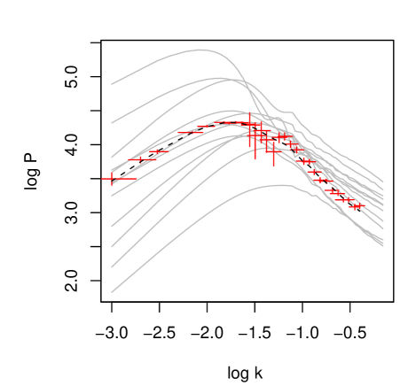
Figure 1: Twenty-eight data points mimicking a combined data set from a large scale structure survey and CMB data. The error bars are chosen to match the power spectrum calculation in Ref. tegmark . The dashed line shows the original input power spectrum from ten realizations, while the gray lines show a subset of the 128 simulated power spectra, discussed in Section II.2.

II.2 The Simulation Design

Ongoing and near-future observations set stringent requirements on the accuracy of theoretical predictions for observables such as the power spectrum and the halo mass function. It will soon be insufficient to use analytic fits for the power spectrum (see, e.g., Refs. PD ; smith03 ) or Press-Schechter like fits (e.g., Refs. PS ; ST ; WAHT ; HLHR ; Reed06 ; Lukic07 ) for the mass function. Fully nonlinear treatments based on simulations will be needed, especially if the aim is to get reliable results on small scales ($k\geq 0.2h^{-1}$Mpc). As discussed earlier, such simulations can be very costly, especially if they are not restricted only to dark matter, but also include gas physics. In addition, the dimensionality of the parameter space to be explored is large, with possibly of order twenty parameters to be considered. This combination of a limited number of simulation runs and a rather large number of cosmological and modeling parameters to be constrained demands a thoughtful design strategy for deciding on the parameter settings at which to run the simulations.

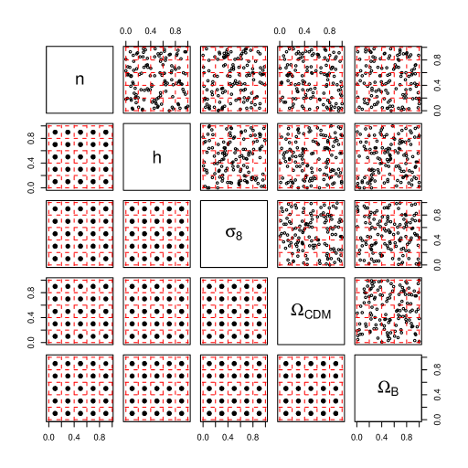
Figure 2: Lower triangle of plots: 2-dimensional projections of a $m=128$ point, 5-level, OA design. Upper triangle: An OA-based LH design obtained by spreading out the 5 level OA design so that each 1-dimensional projection gives an equally spaced set of points along [0,1].

The simulation design refers to a sequence of simulation runs carried out at $m$ input settings which vary over predefined ranges for each of the $p_{\theta}$ input parameters:

$$\begin{pmatrix}\theta_{1}^{*}\\ \vdots\\ \theta_{m}^{*}\end{pmatrix}=\begin{pmatrix}\theta_{11}^{*}&\cdots&\theta_{1p_{\theta}}^{*}\\ \vdots&\vdots&\vdots\\ \theta_{m1}^{*}&\cdots&\theta_{mp_{\theta}}^{*}\end{pmatrix}.$$ (7)

We use $\theta^{*}$ to differentiate the design input settings from the true value of the parameter vector $\theta$ which is to be estimated.

The design of computer experiments, as simulations are often referred to in the statistical literature, has received considerable attention recently in the statistics community, spurred on largely by the increasing use of complex simulation models to augment understanding gained from experiments or observations (see Ref. sant04 , Chs. 5-6, for a recent survey of the area). The goal in our application is to use a sequence of simulation runs to build a GP-based emulator for the expensive simulation code with the aim of predicting code output at untried parameter input settings. A GP model typically interpolates the output of the “training” simulations obtained from the experimental design, and gives predictions that vary smoothly with changes in the input parameters. Because the GP model exploits the smoothness in the simulation response (as a function of the input parameters), space-filling Latin hypercube (LH) designs have proven to be well suited to the purpose of building GP-based emulators welch89 ; ill91 . In particular, we have used orthogonal array (OA)-based LH designs tang as well as symmetric LH designs ye . Fig. 2 shows the $m=128$ point design over the $p_{\theta}=5$ dimensions used in this analysis. This design was constructed by perturbing a 5-level orthogonal array design so that each 1-dimensional projection gives an equally spaced set of points along the standardized parameter range [0,1].

The actual parameter ranges used for the $m=128$ simulations are

$$0.8\leq n \leq 1.4,$$

$$0.5\leq h \leq 1.1,$$

$$0.6\leq \sigma_{8} \leq 1.6,$$

$$0.05\leq \Omega_{\rm CDM} \leq 0.6,$$

$$0.02\leq \Omega_{\rm b} \leq 0.12.$$ (8)

These ranges are standardized to $[0,1]^{5}$ by shifting and scaling each interval. (The resulting simulations are produced by joining spectra obtained from CMBFAST and MC² as described in Section II.1 and as shown in Fig.1.)

Such space filling LH designs are well-suited to the strengths of a GP model which can be fit to an arbitrary set of design points. In contrast, more standard interpolation schemes (e.g., Ref. press99 , Ch. 3.6) typically require a grid-based design for interpolation. Grid-based designs are very inefficient since expanding even a sparse grid over a $p_{\theta}$-dimensional space will be computationally prohibitive. For our example, where $p_{\theta}=5$, even a $[0,\frac{1}{2},1]^{5}$ grid requires 243 simulations. The grid-based approach, while simpler, also gives very poor coverage of low-dimensional projections. In our example, most of the simulator activity is explained by two parameters, $\sigma_{8}$ and $\Omega_{\rm CDM}$, for which the grid-based design assigns only 9 unique values.

II.3 Emulating Simulator Output

Our analysis requires the development of a probability model to describe the simulator output at untried settings $\theta$. To do this, we use the simulator outputs to construct a GP model that “emulates” the simulator at arbitrary input settings over the (standardized) design space $[0,1]^{p_{\theta}}$. To construct this emulator, we model the simulation output using a $p_{\eta}$-dimensional basis representation:

$$\eta(k;\theta)=\sum_{i=1}^{p_{\eta}}\phi_{i}(k)w_{i}(\theta)+\epsilon,\;\theta\in[0,1]^{p_{\theta}},$$ (9)

where $\{\phi_{1}(k),\ldots,\phi_{p_{\eta}}(k)\}$ is a collection of orthogonal, $n_{\eta}$-dimensional basis vectors, the $w_{i}(\theta)$’s are GPs over the input space, and $\epsilon$ is an $n_{\eta}$-dimensional error term. This type of formulation reduces the problem of building an emulator that maps $[0,1]^{p_{\theta}}$ to $R^{n_{\eta}}$ to building $p_{\eta}$ independent, univariate GP models for each $w_{i}(\theta)$. The details of this model specification are given below.

Output from each of the $m$ simulation runs prescribed by the design results in $n_{\eta}$-dimensional vectors, which we denote by $\eta_{1},\ldots,\eta_{m}$. Since the simulations rarely give incomplete output, the simulation output can often be efficiently represented via principal components RamSil97 . We first standardize the simulations by centering about the mean of raw simulation output vectors: $\frac{1}{m}\sum_{j=1}^{m}\eta_{j}$. We then scale the output by a single value so that its variance is 1. This standardization simplifies some of the prior specifications in our models. We also note that, depending on the application, an alternative standardization may be preferred. Whatever the choice of the standardization, the same standardization is also applied to the experimental data.

We define $y_{\rm sims}$ to be the $n_{\eta}\times m$ matrix obtained by column-binding the (standardized) output vectors from the simulations

$$y_{\rm sims}=[\eta_{1};\cdots;\eta_{m}].$$ (10)

Typically, the size of a given simulation output $n_{\eta}$ is much larger than the number of simulations carried out, $m$. We apply the singular value decomposition (SVD) to the simulation output matrix $y_{\rm sims}$ giving

$$y_{\rm sims}=UDV^{T},$$ (11)

where $U$ is a $n_{\eta}\times m$ orthogonal matrix, $D$ is a diagonal $m\times m$ matrix holding the singular values, and $V$ is a $m\times m$ orthonormal matrix. To construct a $p_{\eta}$-dimensional representation of the simulation output, we define the principal component (PC) basis matrix $\Phi_{\eta}$ to be the first $p_{\eta}$ columns of $[\frac{1}{\sqrt{m}}UD]$. The resulting principal component loadings or weights are then given by $[\sqrt{m}V]$, whose columns have variance 1.

For representing the mass power spectrum we found that it is adequate to take $p_{\eta}=5$ so that $\Phi_{\eta}=[\phi_{1};\phi_{2};\phi_{3};\phi_{4};\phi_{5}]$; the basis functions $\phi_{1}$, $\phi_{2}$, $\phi_{3}$, $\phi_{4}$ and $\phi_{5}$ are shown in Fig. 3.

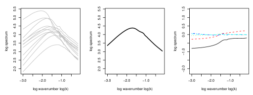
Figure 3: Simulations (left), mean (center), and the first five principal component bases (right) derived from the simulation output for the power spectrum.

Note that the $\phi_{i}$’s are functions of the logarithm of the wave number, $k$.

We use the basis representation of Eqn. (9) to model the $n_{\eta}$-dimensional simulator output over the input space. Each PC weight $w_{i}(\theta)$, $i=1,\dots,p_{\eta}$, is then modeled as a mean-zero GP

$$w_{i}(\theta)\sim\mbox{GP}(0,\lambda^{-1}_{wi}R(\theta,\theta^{\prime};\rho_{wi})),$$ (12)

where $\lambda_{wi}$ is the marginal precision of the process and the correlation function is given by

$$R(\theta,\theta^{\prime};\rho_{wi})=\prod_{l=1}^{p_{\theta}}\rho_{wil}^{4(\theta_{l}-\theta^{\prime}_{l})^{2}}.$$ (13)

This is the Gaussian covariance function, which gives very smooth realizations, and has been used previously in Refs. KOH ; SWMW to model simulation output. An advantage of this product form is that only a single additional parameter is required per additional input dimension, while the fitted GP response still allows for rather general interactions between inputs. We use this Gaussian form for the covariance function because the simulators we work with tend to respond very smoothly to changes in the inputs. Depending on the nature of the sensitivity of simulation output to input changes, one may wish to alter this covariance specification to allow for rougher realizations. The parameter $\rho_{wil}$ controls the spatial range for the $l$th input dimension of the process $w_{i}(\theta)$. Under this parameterization, $\rho_{wil}$ gives the correlation between $w_{i}(\theta)$ and $w_{i}(\theta^{\prime})$ when the input conditions $\theta$ and $\theta^{\prime}$ are identical, except for a difference of 0.5 in the $l$th component. Note that this interpretation makes use of the standardization of the input space to $[0,1]^{p_{\theta}}$.

Restricting to the $m$ input design settings given in Eqn. (7), we define the $m$-vector $w_{i}$ to be the restriction of the process $w_{i}(\cdot)$ to the input design settings

$$w_{i}=(w_{i}(\theta^{*}_{1}),\ldots,w_{i}(\theta^{*}_{m}))^{T},\;\;i=1,\ldots,p_{\eta}.$$ (14)

In addition we define $R(\theta^{*};\rho_{wi})$ to be the $m\times m$ correlation matrix resulting from applying Eqn. (13) to each pair of input settings in the design. The $p_{\theta}$-vector $\rho_{wi}$ gives the correlation distances for each of the input dimensions.

At the $m$ simulation input settings, the $mp_{\eta}$-vector $w=(w_{1}^{T},\ldots,w_{p_{\eta}}^{T})^{T}$ then has prior distribution

$$\begin{pmatrix}w_{1}\cr\vdots\cr w_{p_{\eta}}\end{pmatrix}\sim N\left(\begin{pmatrix}0\cr\vdots\cr 0\end{pmatrix},\begin{pmatrix}\Lambda_{w_{1}}&0&0\cr 0&\ddots&0\cr 0&0&\Lambda_{w_{p_{\eta}}}\end{pmatrix}\right),$$ (15)

$$\Lambda_{w_{i}}\equiv\lambda^{-1}_{w_{i}}R(\theta^{*};\rho_{w_{1}}),$$

which is controlled by $p_{\eta}$ precision parameters held in $\lambda_{w}$ and $p_{\eta}\cdot p_{\theta}$ spatial correlation parameters held in $\rho_{w}$.

The centering of the simulation output makes the choice of zero mean prior appropriate. The prior above can be written more compactly as

$$w\sim N(0,\Sigma_{w}),$$

where $\Sigma_{w}$, controlled by parameter vectors $\lambda_{w}$ and $\rho_{w}$, is given in Eqn. (15).

We specify independent $\Gamma(a_{w},b_{w})$ priors for each $\lambda_{wi}$ and independent beta$(a_{\rho_{w}},b_{\rho_{w}})$ priors for the $\rho_{wil}$’s:

$$\pi(\lambda_{wi}) \propto \lambda_{wi}^{a_{w}-1}e^{-b_{w}\lambda_{wi}},\;\;i=1,\ldots,p_{\eta},$$

$$\pi(\rho_{wil}) \propto \rho_{wil}^{a_{\rho_{w}}-1}(1-\rho_{wil})^{b_{\rho_{w}}-1},\;\;i=1,\ldots,p_{\eta},$$

$$\hskip 108.12054ptl=1,\ldots,p_{\theta}.$$

We expect the marginal variance for each $w_{i}(\cdot)$ process to be close to unity due to the standardization of the simulator output. For this reason we specify that $a_{w}=b_{w}=5$. Thus $\lambda_{wi}$ has a prior mean of 1, and a prior standard deviation of $0.45$. In addition, this informative prior helps stabilize the resulting posterior distribution for the correlation parameters which can be traded off with the marginal precision parameter kern .

Because we expect only a subset of the inputs to influence the simulator response, our prior for the correlation parameters reflects this expectation of “effect sparsity”. Under the parameterization in Eqn. (13), input $l$ is inactive for PC $i$ if $\rho_{wil}=1$. Choosing $a_{{\rho_{w}}}=1$ and $0<b_{{\rho_{w}}}<1$ will give a density with substantial prior mass near 1. We take $b_{\rho_{w}}=0.1$, which makes Pr$(\rho_{wil}<0.98)\approx 1/3$ a priori. In general, the selection of these hyperparameters should depend on how many of the $p_{\theta}$ inputs are expected to be active.

If we take the error vector in the basis representation of Eqn. (9) to be i.i.d. (independent and identically distributed) normal, we can then develop the sampling model, or likelihood, for the simulator output. We define the $n_{\eta}m$-vector $\eta$ to be the concatenation of all $m$ simulation output vectors

$$\eta=\mbox{vec}(y_{\rm sims})=\mbox{vec}([\eta(\theta_{1}^{*});\cdots;\eta(\theta_{m}^{*})]).$$ (16)

Given precision $\lambda_{\eta}$ of the errors, the likelihood is then

$$L(\eta|w,\lambda_{\eta})\propto\lambda_{\eta}^{\frac{mn_{\eta}}{2}}\exp\left\{-\mbox{\small$\frac{1}{2}$}\lambda_{\eta}(\eta-\Phi w)^{T}(\eta-\Phi w)\right\},\;\;$$ (17)

where the $n_{\eta}\times mp_{\eta}$ matrix $\Phi$ is given by

$$\Phi=[I_{m}\otimes\phi_{1};\cdots;I_{m}\otimes\phi_{p_{\eta}}],$$ (18)

and the $\phi_{i}$’s are the $p_{\eta}$ basis vectors previously computed via SVD. A $\Gamma(a_{\eta},b_{\eta})$ prior is specified for the error precision $\lambda_{\eta}$. This parameter controls the size of the errors between the actual simulations and the basis representation of the simulations. We expect the data to be very informative about $\lambda_{\eta}$, so we choose $a_{\eta}=1$ and $b_{\eta}=.0001$, which gives little prior information regarding $\lambda_{\eta}$.

Since the likelihood factors are as shown below

$$L(\eta|w,\lambda_{\eta})\propto$$

$$\lambda_{\eta}^{\frac{mp_{\eta}}{2}}\exp\left\{-\mbox{\small$\frac{1}{2}$}\lambda_{\eta}(w-\hat{w})^{T}(\Phi^{T}\Phi)(w-\hat{w})\right\}\times$$

$$\lambda_{\eta}^{\frac{m(n_{\eta}-p_{\eta})}{2}}\exp\left\{-\mbox{\small$\frac{1}{2}$}\lambda_{\eta}\eta^{T}(I-\Phi(\Phi^{T}\Phi)^{-1}\Phi^{T})\eta\right\},$$

the formulation can be equivalently represented with a dimension-reduced likelihood and a modified $\Gamma(a^{\prime}_{\eta},b^{\prime}_{\eta})$ prior for $\lambda_{\eta}$:

$$L(\hat{w}|w,\lambda_{\eta})\propto$$

$$\lambda_{\eta}^{\frac{mp_{\eta}}{2}}\exp\left\{-\mbox{\small$\frac{1}{2}$}\lambda_{\eta}(\hat{w}-w)^{T}(\Phi^{T}\Phi)(\hat{w}-w)\right\},$$

where

$$a^{\prime}_{\eta} = a_{\eta}+\frac{m(n_{\eta}-p_{\eta})}{2},$$

$$b^{\prime}_{\eta} = b_{\eta}+\mbox{\small$\frac{1}{2}$}\eta^{T}(I-\Phi(\Phi^{T}\Phi)^{-1}\Phi^{T})\eta,\mbox{ and}$$

$$\hat{w} = (\Phi^{T}\Phi)^{-1}\Phi^{T}\eta.$$ (20)

Thus, the normal likelihood for $\eta$ with the gamma prior for $\lambda_{\eta}$

$$\eta|w,\lambda_{\eta}\sim N(\Phi w,\lambda_{\eta}^{-1}I_{n_{\eta}}),\,\lambda_{\eta}\sim\Gamma(a_{\eta},b_{\eta})$$

is mathematically equivalent to a normal model for $\hat{w}$ with an altered gamma-prior model for $\lambda_{\eta}$

$$\hat{w}|w,\lambda_{\eta}\sim N(w,(\lambda_{\eta}\Phi^{T}\Phi)^{-1}),\,\lambda_{\eta}\sim\Gamma(a^{\prime}_{\eta},b^{\prime}_{\eta})$$

since

$$L(\eta|w,\lambda_{\eta})\times\pi(\lambda_{\eta};a_{\eta},b_{\eta})\propto L(\hat{w}|w,\lambda_{\eta})\times\pi(\lambda_{\eta};a^{\prime}_{\eta},b^{\prime}_{\eta}).$$ (21)

The likelihood depends on the simulations only through the computed PC weights $\hat{w}$. After integrating out $w$, the posterior distribution becomes

$$\pi(\lambda_{\eta},\lambda_{w},\rho_{w}|\hat{w})\propto$$

$$\left|(\lambda_{\eta}\Phi^{T}\Phi)^{-1}+\Sigma_{w}\right|^{-\frac{1}{2}}\times$$

$$\exp\{-\mbox{\small$\frac{1}{2}$}\hat{w}^{T}([\lambda_{\eta}\Phi^{T}\Phi]^{-1}+\Sigma_{w})^{-1}\hat{w}\}\times$$

$$\lambda_{\eta}^{a^{\prime}_{\eta}-1}e^{-b^{\prime}_{\eta}\lambda_{\eta}}\prod_{i=1}^{p_{\eta}}\lambda_{wi}^{a_{w}-1}e^{-b_{w}\lambda_{wi}}\prod_{i=1}^{p_{\eta}}\prod_{j=1}^{p_{\theta}}(1-\rho_{wij})^{b_{\rho}-1}.$$

This posterior distribution is a milepost on the way to the complete formulation, which also incorporates experimental data. However, it is well worth further considering this intermediate posterior distribution for the simulator response. It can be explored via MCMC using standard Metropolis updates and we can view a number of posterior quantities to illuminate features of the simulator. For example, Fig. 4 shows boxplots of the posterior distributions for the components of $\rho_{w}$. From this figure it is apparent that PCs 1 and 2 are most influenced by $\sigma_{8}$ and $\Omega_{\rm CDM}$.

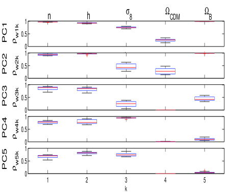
Figure 4: Boxplots of posterior samples for each $\rho_{wil}$ for the mass power spectrum.

Given the posterior realizations from Eqn. (II.3), one can generate realizations from the process $\eta(\theta)$ at any input setting $\theta^{\star}$. Since

$$\eta(k;\theta^{\star})=\sum_{i=1}^{p_{\eta}}\phi_{i}(k)w_{i}(\theta^{\star}),$$ (24)

realizations from the $w_{i}(\theta^{\star})$ processes need to be drawn given the MCMC output. For a given draw $(\lambda_{\eta},\lambda_{w},\rho_{w})$ a draw of $w^{\star}=(w_{1}(\theta^{\star}),\ldots,w_{p_{\eta}}(\theta^{\star}))^{T}$ can be produced by making use of the fact

$$\begin{pmatrix}\hat{w}\cr w^{\star}\end{pmatrix}\sim$$

$$N\left(\begin{pmatrix}0\cr 0\end{pmatrix},\left[\begin{pmatrix}(\lambda_{\eta}\Phi^{T}\Phi)^{-1}&0\cr 0&0\end{pmatrix}+\Sigma_{w,w^{\star}}(\lambda_{w},\rho_{w})\right]\right),$$

where $\Sigma_{w,w^{\star}}$ is obtained by applying the prior covariance rule to the augmented input settings that include the original design and the new input setting $(\theta^{\star})$. [Recall that $\hat{w}$ is defined in Eqn. (20).] Application of the conditional normal rules then gives

$$w^{\star}|\hat{w}\sim N(V_{21}V_{11}^{-1}\hat{w},V_{22}-V_{21}V_{11}^{-1}V_{12}),$$ (26)

where

$$V = \begin{pmatrix}V_{11}&V_{12}\cr V_{21}&V_{22}\end{pmatrix}$$ (27)

$$= \left[\begin{pmatrix}(\lambda_{\eta}\Phi^{T}\Phi)^{-1}&0\cr 0&0\end{pmatrix}+\Sigma_{w,w^{\star}}(\lambda_{w},\rho_{w})\right]$$

is a function of the parameters produced by the MCMC output. Hence, for each posterior realization of $(\lambda_{\eta},\lambda_{w},\rho_{w})$, a realization of $w^{\star}$ can be produced. The above recipe easily generalizes to give predictions over many input settings at once.

Fig. 5 shows posterior means for the simulator response $\eta$ where each of the inputs is varied over its prior range of $[0,1]$ while the other four inputs are held at their nominal setting of 0.5.

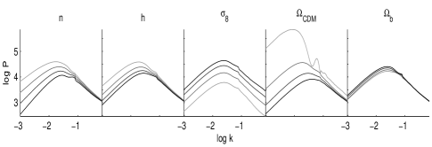
Figure 5: Changes to the posterior mean simulator predictions obtained by varying one input, while holding others at their central values, i.e. at the midpoint of their range. The light to dark lines correspond to the smallest parameter setting to the biggest, for each parameter.

The posterior mean response conveys an idea of how the different parameters affect the highly multivariate simulation output. Other marginal functionals of the simulation response can also be calculated such as sensitivity indicies or estimates of the Sobol decomposition SWMW ; OOH .

Note that a simplified emulator can be constructed by taking point estimates for $(\lambda_{\eta},\lambda_{w},\rho_{w})$ (posterior mean, or posterior medians) and then defining the emulator to be the mean in Eqn. (26).

II.3.1 Emulator Test and Convergence

How do we know that the constructed emulator is accurate and how many model simulations are needed to obtain the desired emulation accuracy? The answers to these questions depend very much on the smoothness of the function we wish to emulate. If the function is smooth and almost featureless, one anticipates that only a small number of simulations should suffice to yield an accceptable emulator. The presence of features and noise in the function to be emulated will clearly require many more simulation outputs; it may well be that beyond some point the optimal emulation strategy is no longer based on the GP model. The number of simulations required to build an accurate emulator depends strongly on the number of active parameters, i.e., parameters that change the output considerably when varied.

To test the accuracy of a proposed emulator, so-called hold-out tests are very useful. The basic idea is simple: A small subset of of the simulations is set aside and the emulator built on the remaining simulations. Then the new emulator is evaluated at the parameter settings of the held-out simulations. By comparing the emulator and simulation results, the accuracy of the emulator can be estimated. An example of this approach is provided in Ref. HHNH where we perform hold-out tests by building the emulator on a subset of 125 out of the total of 128 simulations. Then we test the the emulator on the remaining three simulations by running it at the exact parameter settings of the three holdouts. In this way we test (in turn) the emulator on all 128 simulations.

In the current paper, we present a slightly modified strategy. In addition to the 128 run design, we also employ an independent 64 run design as a reference to investigate the accuracy of the emulator. The present approach has the advantage that the emulator under test is built on the full set of simulations. This might not be too important if the design is already large, but if the design is restricted to a small number of runs, every run is important in determining the accuracy of the emulator, especially near the boundaries of the sampling domain.

In the left panel of Fig. 6 we show the results for the predictions of the 128 run emulator on the additional 64 runs. Overall, the emulator performance is very satisfactory. We display the residuals of the emulator prediction compared to the simulation runs on the native scale. The dark gray band contains the middle 50% of the residuals, the light gray band the middle 90%. The overall accuracy of our emulator over a wide range in wave number is better than $\sim 5$%. Only on the edges of the parameter ranges investigated is the fidelity slightly worse. Note that the emulation accuracy is strongly dependent on the size of the allowed parameter range, and improves significantly as this range is shrunk. We will come back to this point later below.

Next we investigate how the accuracy of the emulator depends on the number of the underlying simulations. We create a design for 32 simulations using an OA-LH sampling design and test it on the same reference 64 design run we already used for testing the 128 run emulator. In Fig. 6, right panel, we show the same statistics as for the 128 run emulator. The overall quality of the emulator is still very good, at the 10% level. Compared with the larger-design emulator, however, the predictions in the medium $k$ range show a higher level of deviation from the reference values.

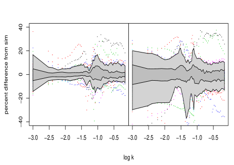
Figure 6: Emulator predictions for a 64 run design. Left: emulator based on 128 runs, right: emulator based on 32 runs. The central gray region contains the middle 50% of the residuals, the wider light gray region, the middle 90%. The outliers are shown as dots. The improvement of the emulator accuracy with more training runs is evident, especially in the medium $k$-range.

II.4 Full Statistical Formulation

Given the model specifications for the simulator $\eta(\theta)$, we can now consider the sampling model for the experimentally observed data. The data are contained in an $n$-vector $y$. For the synthetic mass power spectrum application, $n=28$, corresponding to the different wave numbers as shown in Fig. 1. As stated in Section II, the data are modeled as a noisy version of the simulated spectrum $\eta(k;\theta)$ run at the true, but unknown, parameter setting $\theta$, $y=\eta(k;\theta)+\epsilon,$ where the errors are assumed to be $N(0,\Sigma_{y})$. For notational convenience we represent $\Sigma_{y}^{-1}$ as $\lambda_{y}W_{y}$, leaving open the option to estimate a scaling of the error covariance with $\lambda_{y}$. Using the basis representation for the simulator this becomes

$$y = \Phi_{y}w(\theta)+\epsilon,$$

where $w(\theta)$ is the $p_{\eta}$-vector $(w_{1}(\theta),\ldots,w_{p_{\eta}}(\theta))^{T}$. Because the wave number support of $y$ is not necessarily contained in the support of the simulation output, the basis vectors in $\Phi_{y}$ may have to be interpolated over wave number from $\Phi_{\eta}$. Since the simulation output over wave number is quite dense, this interpolation is straightforward.

We specify a $\Gamma(a_{y},b_{y})$ prior for the precision parameter $\lambda_{y}$ resulting in a normal-gamma form for the data model

$$y|w(\theta),\lambda_{y}\sim N(\Phi_{y}w(\theta),(\lambda_{y}W_{y})^{-1}),\,\lambda_{y}\sim\Gamma(a_{y},b_{y}).$$ (28)

The observation precision $W_{y}$ is often fairly well-known in practice. Hence one may choose to fix $\lambda_{y}$ at 1, or use an informative prior that encourages its value to be near one. In the mass power spectrum example we fix $\lambda_{y}$ at 1, though we continue to use this parameter in the formulation below.

Equivalently, Eqn. (28) can be represented in terms of the basis weights

$$\hat{w}_{y}|w(\theta),\lambda_{y}\sim N(w(\theta),(\lambda_{y}\Phi_{y}^{T}W_{y}\Phi_{y})^{-1}),\;\lambda_{y}\sim\Gamma(a^{\prime}_{y},b^{\prime}_{y}),$$ (29)

with

$$\hat{w}_{y} = (\Phi_{y}^{T}W_{y}\Phi_{y})^{-1}\Phi_{y}^{T}W_{y}y,$$

$$a^{\prime}_{y} = a_{y}+\mbox{\small$\frac{1}{2}$}(n-p_{\eta}),\mbox{ and}$$

$$b^{\prime}_{y} = b_{y}+\mbox{\small$\frac{1}{2}$}(y-\Phi_{y}\hat{w}_{y})^{T}W_{y}(y-\Phi_{y}\hat{w}_{y}).$$

This equivalency follows from Eqn. (21) given in Sec. II.3.

The (marginal) distribution for the combined, reduced data obtained from the experiments and simulations given the covariance parameters, has the form

$$\begin{pmatrix}\hat{w}_{y}\cr\hat{w}\end{pmatrix}\sim\mbox{N}\left(\begin{pmatrix}0\cr 0\end{pmatrix},\begin{pmatrix}\Lambda_{y}^{-1}&0\cr 0&\Lambda_{\eta}^{-1}\end{pmatrix}+\begin{pmatrix}I_{p_{\eta}}&\Sigma_{w_{y}w}\cr\Sigma_{w_{y}w}^{T}&\Sigma_{w}\end{pmatrix}\right),$$ (30)

where $\Sigma_{w}$ is defined in (15),

$$\Lambda_{y} = \lambda_{y}\Phi_{y}^{T}W_{y}\Phi_{y},$$

$$\Lambda_{\eta} = \lambda_{\eta}\Phi^{T}\Phi,$$

$$I_{p_{\eta}} = p_{\eta}\times p_{\eta}\mbox{ identity matrix},$$

$$\Sigma_{w_{y}w} = \begin{pmatrix}\lambda^{-1}_{w1}R(\theta,\theta^{*};\rho_{w1})&0&0\\ 0&\ddots&0\\ 0&0&\lambda^{-1}_{wp_{\eta}}R(\theta,\theta^{*};\rho_{wp_{\eta}})\end{pmatrix}.$$

Above, $R(\theta,\theta^{*};\rho_{wi})$ denotes the $1\times m$ correlation submatrix for the GP modeling the simulator output obtained by applying Eqn. (13) to the observational setting $\theta$ crossed with the $m$ simulator input settings $\theta^{*}_{1},\ldots,\theta^{*}_{m}$.

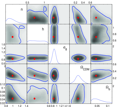
Figure 7: Estimated posterior distribution of the parameters $\theta=(n,h,\sigma_{8},\Omega_{\rm CDM},\Omega_{\rm b})$. The diagonal shows the estimated marginal posterior pdf for each parameter; the off-diagonal images give estimates of bivariate marginals; the contour lines show estimated 90% hpd regions. The true values from which the data were generated are shown by the red dots.

II.4.1 Posterior distribution

If we take $\hat{z}$ to denote the reduced data $(\hat{w}^{T}_{y},\hat{w}^{T})^{T}$, and $\Sigma_{\hat{z}}$ to be the covariance matrix given in Eqn. (30), the posterior distribution has the form

$$\pi(\lambda_{\eta},\lambda_{w},\rho_{w},\lambda_{y},\theta|\hat{z})\propto$$

$$|\Sigma_{\hat{z}}|^{-\frac{1}{2}}\exp\left\{-\mbox{\small$\frac{1}{2}$}\hat{z}^{T}\Sigma_{\hat{z}}^{-1}\hat{z}\right\}\times$$

$$\lambda_{\eta}^{a^{\prime}_{\eta}-1}e^{-b^{\prime}_{\eta}\lambda_{\eta}}\prod_{i=1}^{p_{\eta}}\lambda_{wi}^{a_{w}-1}e^{-b_{w}\lambda_{wi}}\times$$

$$\prod_{i=1}^{p_{\eta}}\prod_{l=1}^{p_{\theta}}\rho_{wil}^{a_{\rho_{w}}-1}(1-\rho_{wil})^{b_{\rho_{w}}-1}\lambda_{y}^{a^{\prime}_{y}-1}e^{-b^{\prime}_{y}\lambda_{y}}I[\theta\in C],$$

where $C$ denotes the constraint region for $\theta$, which is typically a $p_{\theta}$-dimensional rectangle. In other applications $C$ can also incorporate constraints between the components of $\theta$.

Realizations from the posterior distribution are produced using standard, single site MCMC. Metropolis updates metrop are used for the components of $\rho_{w}$ and $\theta$ with a uniform proposal distribution centered at the current value of the parameter. The precision parameters $\lambda_{\eta}$, $\lambda_{w}$ and $\lambda_{y}$ are sampled using Hastings updates hastings . Here the proposals are uniform draws, centered at the current parameter values, with a width that is proportional to the current parameter value. In a given application the candidate proposal width can be tuned for optimal performance.

The resulting posterior distribution estimate for $\theta$ is shown in Fig. 7 on the original scale. It nicely brackets the true values of $\theta=(0.99,0.71,0.84,0.27,0.044)$ from which the synthetic data were generated.

III Combined CMB and large scale structure analysis

So far our analysis has focused on a single observational data set, but cosmological parameter estimation requires combining a number of different observational datasets with their (separate) associated modeling methodologies. We now consider a simple example of this, the joint analysis of CMB temperature anisotropy data and the mass power spectrum as sampled by large-scale structure surveys.

The power spectrum of the CMB anistropy as a function of angular scale or multipole moment $l$ has significantly more structure than the matter power spectrum and therefore presents a more challenging test for our framework. In this section we extend our synthetic data set to include these measurements. We restrict our analysis to the six-dimensional “vanilla” $\Lambda$CDM model described by

$$\theta=(n,h,\sigma_{8},\Omega_{\rm CDM},\Omega_{\rm b},\tau).$$ (32)

Different groups analyzing different data sets, e.g. Refs. spergel ; tegmark06 , found that the model specified by these six parameters consistently fits all currently available data. Our synthetic data set mimics data from WMAP-III spergel and the galaxy mass power spectrum from the SDSS tegmark . For the synthetic dataset, we choose the same cosmology as given in Eqn. (6) and in addition the optical depth:

$$\tau=0.09.$$ (33)

We allow $\tau$ to vary between 0 and 0.3 in our analysis below. The analysis of the CMB data was carried out using the CAMB camb code throughout. We have carefully checked that the transfer functions generated with CMBFAST for the $N$-body simulations agree very accurately with the CAMB transfer functions. Our synthetic data set allows us to ignore real-world corrections such as for the normalization from the Sunyaev-Zel’dovich effect due to hot gas in clusters. The WMAP-III analysis showed that such considerations can become important for precision measurements of cosmological parameters.

III.1 Constraints from the Cosmic Microwave Background

Before we carry out a combined analysis of galaxy survey and CMB data, we investigate how well our framework does in dealing with the CMB temperature angular power spectrum (TT). We do not consider CMB polarization here but there is no obstacle to including it in future studies.

As done earlier for the matter power spectrum we generate a synthetic data set for the TT spectrum. For the error bars we assume the same magnitude as in the WMAP-III analysis. We first run CAMB at the parameter settings specified in Eqns. (6) and (33) and then move the data points off the base TT spectrum according to a Gaussian distribution with 1-$\sigma$ confidence level. Following the matter power spectrum analysis we create a design for 128 runs, this time for a six-parameter space. In Fig. 8 we show the analog to Fig. 1 for the TT spectrum: the gray lines show a subset of the 128 CAMB runs, the dashed line the actual input power spectrum and the red points the data points which will be used for our analysis.

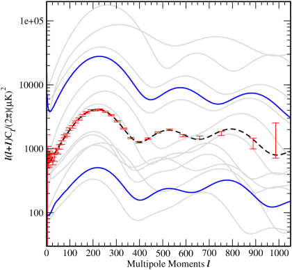
Figure 8: Subset of 128 simulated TT power spectra (gray lines) along with the synthetic observations. The dashed line shows the actual spectrum from which the data were generated. The blue lines show the limits of the restricted parameter ranges from Eqns. (III.1).

In Fig. 9 we show the analog to Fig. 6, demonstrating that the $C_{l}$ emulator predicts 90% of the holdout runs to better than 10% and 50% of the runs to better than 5%. This accuracy is impressive considering the dynamic range and complexity of the $C_{l}$s (and the broad range over which the cosmological parameters are varied). However, this complexity requires more PCs for accurate emulation. We have kept twelve PCs for the $C_{l}$ analysis compared to five PCs for the matter power spectrum analysis. The bivariate marginal plot summarizing the inference in the cosmological parameters taking into account the TT spectrum alone is given in Fig. 10 (compare to Fig. 7).

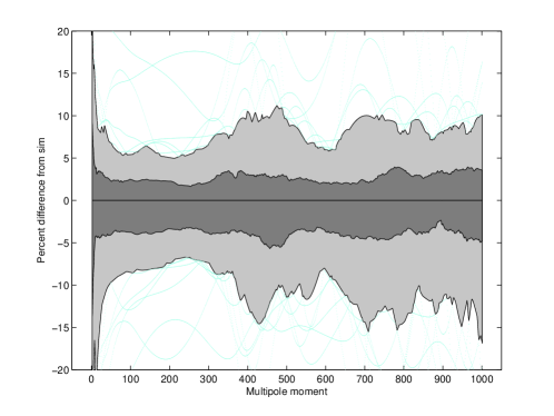
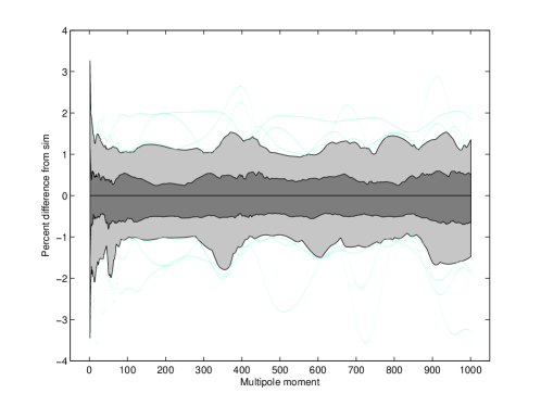
Figure 9: Emulator performance on holdout test. The central gray region contains the middle 50% of the residuals, the wider light gray region, the middle 90%. The outliers are shown as blue curves. Upper plot: Residuals for the emulator built on the conservative priors given in Eqns. (II.2). Lower plot: Residuals for the emulator built on 3-$\sigma$ priors around the best-fit WMAP-III parameters. The emulator errors are reduced by an order of magnitude for the smaller parameter ranges.

Other groups who have developed interpolation schemes to predict the temperature power spectrum kap02 ; Jim04 ; kos02 ; fendt06 ; auld06 choose much narrower priors than we have in our example. If, as is typical, we reduce the parameter ranges to 3-$\sigma$ around the best-fit WMAP data, leading to:

$$0.85\leq n \leq 1.25,$$

$$0.6\leq h \leq 0.9,$$

$$0.6\leq \sigma_{8} \leq 1.2,$$

$$0.06\leq \Omega_{\rm CDM}h^{2} \leq 0.2,$$

$$0.018\leq \Omega_{\rm b}h^{2} \leq 0.034,$$

$$0.01\leq \tau \leq 0.55,$$ (34)

the dynamic range of the $C_{l}$s is in turn reduced by an order of magnitude (blue lines in Fig. 8). This leads to an improvement of the emulator quality by an order of magnitude to yield results at sub-percent level accuracy (Fig. 9, lower panel). We stress that our parameter ranges in this case are still larger than what is considered by other groups. Their procedures are restricted to be valid at 3-$\sigma$ around the best-fit WMAP model, covering only a small range in parameter space. We compare our method with the other approaches in more detail in Appendix A.

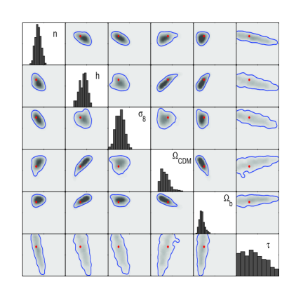
Figure 10: Estimated posterior distribution following Fig. 7 for the synthetic CMB TT spectrum and including the optical depth $\tau$.

III.2 Combined Constraints

We now proceed to systematically combine information contained in the TT and matter power spectra. Given two sets of observed data, $y_{1}$ and $y_{2}$ that inform on a common set of parameters, $\theta$, the posterior density is

$$\pi(\theta|y_{1},y_{2})\propto L(y_{1},y_{2}|\theta)\cdot\pi(\theta).$$ (35)

Assuming statistical independence of the two datasets, the likelihood factors into:

$$\pi(\theta|y_{1},y_{2})\propto L(y_{1}|\theta)\cdot L(y_{2}|\theta)\cdot\pi(\theta),$$ (36)

which is the form we have incorporated into our statistical analysis code.

The payoff from including both sets of observational data is illustrated in Figs. 11 and 12 and in Table 1. The posterior volume of the cosmological parameter space is significantly reduced by the addition of the matter power spectrum constraints. There are two main reasons for this volumetric reduction. First is the expected statistical increase due to the addition of two independent and consistent pieces of data. Second, and more interesting, is the influence of posterior correlations among the cosmological parameters induced by the two datasets. For example, the degeneracy between $n$ and $\tau$ allows the inclusion of matter power spectrum data (the simulations of which are independent of $\tau$) to significantly improve the estimation of $\tau$.

Table 1: Parameter constraints (mean value $\pm$ 1 standard deviation) for six parameters from CMB TT power spectrum analysis alone and with the adddition of large scale structure data. The first line gives the true value of the parameters.

	$n$	$h$	$\sigma_{8}$	$\Omega_{\rm CDM}$	$\Omega_{\rm b}$	$\tau$
Truth	0.99	0.71	0.84	0.27	0.044	0.09
CMB only	1.0185 $\pm$ 0.0422	0.7527 $\pm$ 0.0544	0.8824 $\pm$ 0.1004	0.2387 $\pm$ 0.0592	0.0397$\pm$ 0.006	0.1241 $\pm$ 0.0763
CMB + LSS	1.0090$\pm$ 0.0263	0.7335 $\pm$ 0.0371	0.8722 $\pm$ 0.0262	0.2560 $\pm$ 0.0387	0.0413 $\pm$ 0.0044	0.0922 $\pm$ 0.0434

It is easy to see that including additional datasets into this method is straightforward.

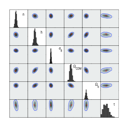
Figure 11: Estimated posterior distribution following Fig. 10 with the addition of matter power spectrum data.

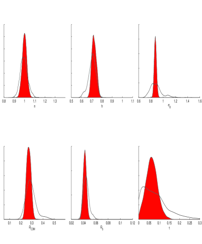
Figure 12: Posterior univariate marginal density estimates for the cosmological parameters taking into account the TT only data (white) and both the TT and the matter power spectrum data (orange), showing the increased precision obtainable by systematically including multiple sources of data.

IV Discussion and Conclusion

We have demonstrated a powerful and general statistical methodology for performing computer simulation-based inference of cosmological parameters. To do this, we borrow techniques from a variety of statistical fields – including experimental design, spatial statistics and Kriging, and Bayesian inference – and apply them in a highly integrated manner to the problem of constraining computational models directly from the observed data. Several items are particularly noteworthy. First, careful simulation design prevents combinatorial explosions of simple grid-like designs in highly multivariate environments. Second, the GP-based emulator design is critical to the efficient sampling of the posterior probability density and allows us to evaluate global measures of the simulator sensitivity cheaply and accurately. Finally, our method isolates the separate sources of uncertainty in any particular inference, e.g., the uncertainty due to imperfect emulation, and folds them into the overall inference uncertainty. This procedure has the conceptual advantage of coherence and the practical advantage of guarding against overly optimistic parameter estimates. It can be easily extended to very large parameter spaces and to include different data sources such as CMB and large scale structure measurements.

Depending on the parameter ranges considered, our emulation scheme can perform at the sub-percent level accuracy, thereby, at least in principle, satisfying a fundamental requirement for next-generation cosmological analysis tools. It is especially suited to – and designed for – problems where the underlying simulations are very costly and only a limited number can be performed. While clearly of more general utility, our framework is targeted to analysis of upcoming large-scale structure based probes of dark energy, such as weak lensing and baryon acoustic oscillations. Future directions and the usage for our framework in cosmology are manifold. We plan to extend the set of cosmological parameters under consideration to include the dark energy equation of state parameter $w$ and to publicly release an emulator scheme based on very accurate, high-resolution dark matter simulations. The framework can also be used to fit supernova light-curves or determine photometric galaxy redshifts based on training sets. Work in this direction is already in progress.

Appendix A Comparison with other methods

In this Appendix we compare the performance of our emulator for the TT power spectrum with other recently introduced interpolation schemes. An early attempt is based on the idea of splitting the TT power spectrum into low-$l$ ($l\leq 100$) and high-$l$ regions ($l\geq 100$) and to use analytic fits to express the $C_{l}$s teg00 . This method is accurate at the 10% level and forms the basis of the approach underlying DASh (Davis Anisotropy Shortcut) developed in Ref. kap02 . DASh relies on rapid analytic and semi-analytic approximations and leads to good accuracy (at the 2% level on average) and performance. Another interpolation scheme, CMBwarp Jim04 , is based on introducing a new set of cosmological parameters (for details on these parameter choices see Ref. kos02 ) which better reflect the underlying physics of the CMB. The degeneracy structure in the new parameter space is much simpler and therefore helps with MCMC convergence. The new parameter set has almost-linear influence on the TT power spectrum (i.e., the spectrum moves mainly vertically or horizontally with parameter changes). It is therefore relatively easy to find a polynomial fit around a fiducial model that is reliable for different parameters. CMBwarp is faster than DASh at the same level of accuracy. Both approaches have two major drawbacks: they only lead to accurate results in a narrow parameter range around a fiducial model and incorporation of new parameters is very difficult since new fits have to be developed. In the case of CMBwarp, any additional parameter has to be “orthogonal” to the others, which might be difficult to achieve. Very recently, a new interpolation method, Pico, was introduced in Ref. fendt06 . Pico is based on a large number of training sets (a $\sim 10^{4}$ run MCMC chain). It allows very accurate and very fast determination of temperature power spectra around the best-fit WMAP model. Pico is trained to compute the power spectra within several log likelihoods around the peak. Therefore, good performance away from the peak cannot be guaranteed. Integration of new parameters is possible by generating new training data sets. Very similar to the Pico approach is CosmoNet auld06 . In this approach, a neural network is trained on 2,000 CAMB runs. The CosmoNet results are very similar in accuracy and speed to Pico.

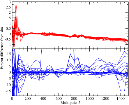
Figure 13: Residuals for the Pico emulator of the TT power spectrum, tested on 64 runs. The upper plot in red shows the residuals for runs which are in the 3-$\sigma$ confidence level around the best-fit WMAP-I model. 22 out of the 64 runs fulfill this criterion. The residuals are at the 0.5% accuracy level in this case. Note the slight downward trend in all cases. The lower plot in blue shows the remaining 42 runs which are in the 3-$\sigma$ confidence level around the best fit parameters from WMAP. In this case the errors are much worse and the emulator is not controlled. Again a slight downward trend can be seen in all the runs.

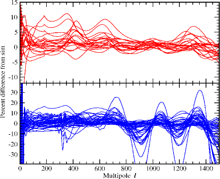
Figure 14: Results following Fig. 13 but for the CMBwarp emulator. The errors are overall an order of magnitude bigger than for Pico, in agreement with the findings of Ref. fendt06 .

We concentrate our comparison on two publicly available codes: CMBwarp and Pico. Both codes are designed to yield reliable, accurate results within WMAP’s first-year 3-$\sigma$ confidence region around the best-fit model. The parameter ranges we have investigated so far are much broader. Therefore, in order to be able to carry out a meaningful comparison between the three different approaches, we build a new emulator based on 128 CAMB runs in the parameter range specified in Eqn. (III.1). (Note that we now also include $h^{2}$ in our variable choice for the dark matter and baryon content of the Universe). These parameter ranges are within 3-$\sigma$ about the best fit parameters, which is still a larger range than Pico and CMBwarp allow. In fact, their allowed ranges are rather narrow and cannot be cast in the form of a symmetric box around the best fit parameters.

In addition to the 128 training runs we generate 64 reference CAMB runs for testing our emulator as well as CMBwarp and Pico. In Fig. 13 we show the emulator quality for Pico. Only 22 out of the 64 simulations lie in the allowed parameter range; we display the residuals for these runs in the upper part of Fig. 13 in red. The accuracy in this parameter range is very good, at the 0.5% level. Somewhat worrisome though is the existence of a systematic trend in the Pico data: All residuals are systematically low for large $l$, possibly leading to biases in the parameter constraints. In the lower plot of Fig. 13 we show the residuals for the remaining 42 simulations in blue, which lie in the 3-$\sigma$ interval around the best fit parameters but not the best fit model for WMAP-I. Here the errors are much bigger, by more than an order of magnitude. This shows that Pico should not be taken out of the parameter range it was trained for, and is not robust against extrapolation into larger parameter ranges (as expected for a polynomial-based fit). Fig. 14 shows the residuals for the CMBwarp runs. As for Pico we have divided them into runs which are inside the 3-$\sigma$ confidence level around the best fit model and those outside, but still inside the 3-$\sigma$ confidence level of the best fit parameters. In general, the performance of CMBwarp is an order of magnitude worse than the performance of Pico, confirming the results in Ref. fendt06 . For $l>180$, the fit is slightly modified, leading to a small kink at this value in the results for the $C_{l}$s. The performance on all 64 runs of our emulator scheme based on GP models is shown in Fig. 9. 50% of all runs are predicted with sub-percent accuracy, 90% with an accuracy between one and two percent. Not a single prediction is off by more than 3%. This demonstrates impressively the stability of our emulator scheme over large parameter ranges.

References

- (1) G.F. Smoot et al., Astrophys. J. 396, L1 (1992).
- (2) B.S. Mason et al., Astrophys. J. 591, 540 (2003).
- (3) N.W. Halverson et al., Astrophys. J. 568, 38 (2002).
- (4) C.L. Kuo et al. [ACBAR collaboration], Astrophys. J. 600, 32 (2004).
- (5) J.E. Ruhl et al., Astrophys. J. 599, 786 (2003).
- (6) A. Benoit et al. [Archeops Collaboration], Astron. Astrophys. 399, L19 (2003).
- (7) D.N. Spergel et al., arXiv:astro-ph/0603449.
- (8) http://www.rssd.esa.int/index.php?project=Planck
- (9) J.E. Gunn et al., Astron. J. 131, 2332 (2006).
- (10) M. Tegmark et al., Phys. Rev. D 74, 123507 (2006).
- (11) D.J. Eisenstein et al. [SDSS Collaboration], Astrophys. J. 633, 560 (2005), and references therein.
- (12) K.N. Abazajian and S. Dodelson, Phys. Rev. Lett. 91, 041301 (2003); B. Jain and A. Taylor, Phys. Rev. Lett. 91, 141302 (2003) and references therein.
- (13) S. Majumdar and J.J. Mohr, Astrophys. J. 613, 41 (2004) and references therein.
- (14) V. Lukash, Pis’ma Zh. Eksp. Teor. Fiz. 31, 631 (1980) [JETP Lett. 31, 596 (1980)]; V.F. Mukhanov and G.V. Chibisov, Pis’ma Zh. Eksp. Teor. Fiz. 33, 549 (1981); A.H. Guth and S.-Y. Pi, Phys. Rev. Lett. 49, 1110 (1982); S.W. Hawking, Phys. Lett. B 115, 295 (1982); A.A. Starobinsky, Phys. Lett. B 117, 175 (1982).
- (15) S. Habib, K. Heitmann, G. Jungman, and C. Molina-Paris, Phys. Rev. Lett. 89, 281301 (2002); S. Habib, A. Heinen, K. Heitmann, G. Jungman, and C. Molina-Paris, Phys. Rev. D 70, 083507 (2004) S. Habib, A. Heinen, K. Heitmann, and G. Jungman, Phys. Rev. D 71, 043518 (2005); and references therein.
- (16) G. Efstathiou and J.R. Bond, Mon. Not. Roy. Astron. Soc. 304, 75 (1999).
- (17) U. Seljak and M. Zaldarriga, Astrophys. J. 469, 437 (1996).
- (18) A. Lewis, A. Challinor, and A. Lasenby, Astrophys. J. 538, 473 (2000).
- (19) M. Tegmark and M. Zaldarriaga, Astrophys. J. 544, 30 (2000).
- (20) R. Jimenez, L. Verde, H. Peiris, and A. Kosowsky, Phys. Rev. D 70, 023005 (2004).
- (21) M. Kaplinghat, L. Knox, and C. Skordis, Astrophys. J. 578, 665 (2002).
- (22) C. Fendt and B. Wandelt, Astrophys. J. 654, 2 (2007).
- (23) T. Auld, M. Bridges, M.P. Hobson, and S.F. Gull, arXiv:astro-ph/0608174.
- (24) R.E. Smith et al. [The Virgo Consortium Collaboration], Mon. Not. Roy. Astron. Soc. 341, 1311 (2003).
- (25) J.A. Peacock and S.J. Dodds, Mon. Not. Roy. Astron. Soc. 267, 1020 (1994).
- (26) http://www.lsst.org
- (27) http://pan-starrs.ifa.hawaii.edu
- (28) http://universe.nasa.gov/program/probes/jdem.html
- (29) Y.P. Jing, P. Zhang, W.P. Lin, L. Gao, and V. Springel, Astrophys. J. 640, L119 (2006).
- (30) D. Rudd et al., in preparation.
- (31) M.S. Warren and J.K. Salmon, in Supercomputing ’93, 12, Los Alamitos IEEE Comp. Soc. (1993).
- (32) K. Heitmann, D. Higdon, C. Nakhleh, and S. Habib, Astrophys. J. 646, L1 (2006).
- (33) M.C. Kennedy and A. O’Hagan, J. Royal Stat. Soc. B 63, Part 3, 425 (2001).
- (34) M. Goldstein and J. Rougier, SIAM J. Sci. Comput. 26, 467 (2004).
- (35) K. Heitmann, P.M. Ricker, M.S. Warren, and S. Habib, Astrophys. J. Supp. 160, 28 (2005).
- (36) J.K. Adelman-McCarthy et al., Astrophys. J. Supp. 162, 38 (2006).
- (37) M. Tegmark et al., Phys. Rev. D, 69, 103501 (2004).
- (38) W.H. Press and P. Schechter, Astrophys. J. 187, 425 (1974).
- (39) R.K. Sheth and G. Tormen, Mon. Not. Roy. Astron. Soc. 308, 119 (1999).
- (40) M.S. Warren, K. Abazajian, D.E. Holz, and L. Teodoro, Astophys. J. 646, 881 (2006).
- (41) K. Heitmann, Z. Lukić, S. Habib, and P.M. Ricker, Astrophys. J. 642, L85 (2006).
- (42) D. Reed, R. Bower, C. Frenk, A. Jenkins, and T. Theuns, Mon. Not. Roy. Astron. Soc. 374, 2 (2007).
- (43) Z. Lukić, K. Heitmann, S. Habib, S. Bashinsky, and P.M. Ricker, in preparation.
- (44) T.J. Santner, B.J. Williams, and W.I. Notz, The Design and Analysis of Computer Experiments, Springer, New York (2003).
- (45) J. Sacks, W.J. Welch, and T.J. Mitchell, Stat. Sci. 4, 409 (1989).
- (46) C. Currin, T. Mitchell, M. Morris, and D. Ylvisaker, J. Am. Stat. Assn. 86, 953 (1991).
- (47) B. Tang, J. Am. Stat. Assn. 88, 1392 (1993).
- (48) K.Q. Ye, W. Li, and A. Sudjianto, J. Stat. Planning and Inference 90, 145 (2000).
- (49) W.H. Press, S.A. Teukolsky, W.T. Vetterling, and B.P. Flannery, Numerical Recipes in Fortran77, The Art of Scientific Computing, 2nd ed., Cambridge University Press (1999).
- (50) J.O. Ramsay and B.W. Silverman, Functional Data Analysis, Springer, New York (1997).
- (51) J. Sacks, W.J. Welch, T.J. Mitchell, and H.P. Wynn, Stat. Sci. 4, 409 (1989).
- (52) J. Kern, Baysian process-convolution approaches to specifying spatial dependence structure, Ph.D. Thesis, Institute of Statistics and Decision Science, Duke University (2000).
- (53) J.E. Oakley and A. O’Hagan, J. R. Stat. Soc. Ser. B-Stat. Methodol. 66, 751 (2004).
- (54) N. Metropolis, A.W. Rosenbluth, M.N. Rosenbluth, A.H. Teller, and E. Teller, J. Chem. Phys. 21, 1087 (1953).
- (55) W.K. Hastings, Biometrika 57, 97 (1970).
- (56) A. Kosowsky, M. Milosavljevic, and R. Jimenez, Phys. Rev. D 66, 063007 (2002).