A Radiation Driven Implosion Model
for the Enhanced Luminosity of Protostars near HII Regions

Abstract

Context. Molecular clouds near the H ii regions tend to harbor more luminous protostars.

Aims. Our aim in this paper is to investigate whether or not radiation-driven implosion mechanism enhances luminosity of protostars near regions of high-ionizing fluxes.

Methods. We performed numerical simulations to model collapse of cores exposed to UV radiation from O stars. We investigated dependence of mass loss rates on the initial density profiles of cores and variation of UV fluxes. We derived simple analytic estimates of accretion rates and final masses of protostars.

Results. Radiation-driven implosion mechanism can increase accretion rates of protostars by 1-2 orders of magnitude. On the other hand, mass loss due to photo-evaporation is not large enough to have a significant impact on the luminosity. The increase of accretion rate makes luminosity 1-2 orders higher than those of protostars that form without external triggering.

Conclusions. Radiation-driven implosion can help explain the observed higher luminosity of protostars in molecular clouds near H ii regions.

1 Introduction

Massive stars play a very important role in star formation history in giant molecular clouds. Strong radiation from massive stars impacts on surrounding environment, and may trigger star formation nearby. Two scenarios of triggered star formation near H ii regions have been suggested. One of them is “collect and collapse” (Elmegreen & Lada, 1977; Whitworth et al., 1994). As the H ii region expands, it pushes ambient gas into a shell. Subsequent fragmentation and collapse of the swept-up shell may form the next generation of stars. For example, a core within one fragment of the molecular ring surrounding Galactic H ii region Sh104 contains a young cluster (Deharveng et al., 2003). Radiation-driven implosion (hereafter, RDI) is the other scenario (Bertoldi, 1989; Bertoldi & McKee, 1990). When an expanding H ii region engulfs a cloud core, the strong UV radiation will compress the core. Bright-rimmed clouds of cometary shapes found at the edges of relatively old H ii regions, are explained by Lefloch & Lazareff (1994) with a RDI model. To understand star formation in giant molecular clouds, we study effects of the RDI.

Observational results indicate that the H ii regions can strongly affect star formation nearby. Dobashi et al. (2001) investigated the maximum luminosity of protostars as a function of the parent cloud mass. They found that molecular clouds near H ii regions contain more luminous protostars than others. Moreover, Sugitani et al. (1989) showed that the ratios of luminosity of protostar to core mass of bright-rimmed globules are much higher than those in dark globules. These results indicate that the RDI affects the luminosity of protostars near H ii region.

Recent studies suggest that triggered star formation by external compression can increase accretion rates and luminosity of protostars. Motoyama & Yoshida (2003) investigated collapses of cores compressed by external shock waves and found that accretion rates were enhanced. Some observations support this result. Belloche et al. (2006) observed the Class 0 protostar IRAS 4A in star formation cloud NGC1333, whose star formation is suspected to be triggered by powerful molecular outflows (Sandell & Knee, 2001). They showed a numerical model of collapse triggered by external pressure, which reproduces the observed density and velocity profiles. Moreover, they deduced a high accretion rate of $(0.7-2)\times 10^{-4}\ \mathrm{M_{\sun}yr^{-1}}$. Their result indicates external compression increases the accretion rate of a protostar, which produces high accretion luminosity. In this paper, we attribute the origin of higher luminosity in protostars to star formation activities induced by the RDI.

Some studies have been made on RDI. Bertoldi (1989) and Bertoldi & McKee (1990) developed an approximate analytical solution for the evolution of a cloud exposed to ionizing UV radiation. Lefloch & Lazareff (1994) investigated the RDI with numerical simulations. However, their calculations did not include self-gravity of the gas. Recently, SPH simulations including self-gravity have been done. Kessel-Deynet & Burkert (2003) investigated the effects of initial density perturbations on the dynamics of ionizing clouds, and Miao et al. (2006) focused on cloud morphology. Despite of many studies on RDI, little attention has been given to the effects of RDI on accretion rates.

In this paper, we explore if the RDI can enhance accretion rates by orders of magnitude compared with those of protostars that form without external trigger. RDI is expected to enhance the accretion rates as a result of strong compression, and it would increase luminosity of protostars. On the other hand, photo-evaporation of the parent core due to RDI decreases the mass of protostar, subsequently decrease the luminosity of the new protostar. We investigate which effect dominates.

The paper is organized as follows. In Section 2, we describe our numerical method. In Section 3, we present our results. In Section 4, we discuss luminosities of protostars based on our numerical results. In Section 5, we summarize our main conclusions.

2 Numerical Method

We simulate evolution of cores exposed to diffuse UV radiation. We assumed that a core of neutral gas is immersed within an H ii region and is exposed to diffuse radiation from the surrounding ionized gas. In an actual H ii region, the core is not only exposed to diffuse radiation but also to direct radiation from the ionizing star. The diffuse flux of Lyman continuum photons is $\sim 15\%$ of the direct flux of Lyman continuum photons (Canto et al., 1998; Whitworth & Zinnecker, 2004). The spherical core has an effective cross-section to diffuse radiation $4\pi r^{2}$ and to direct UV radiation $\pi r^{2}$, respectively. The ratio of total number of diffuse photons to total number of direct photons is $\sim 0.6$. Our assumption underestimates the total amount of ionizing UV photons by a factor of $\sim 2.6$. Since the purpose of this paper is to investigate the effects of RDI on the accretion rate of a protostar, we neglected direct radiation and considered only diffuse radiation for simplicity. Effects of direct radiation and morphology of the core, are beyond the purpose of the present paper, and will be discussed in our next paper using two dimensional simulations.

The ionizing UV photons enter from outer boundary of the computational domain. The number flux of these UV photons is expressed as

$$F_{i}=0.15\times\frac{N_{L}}{4\pi d^{2}},$$ (1)

where $N_{L}$ is the total flux of ionizing UV photons from the star, and $d$ is distance from the ionizing star to the core. We assume that the ionizing star is an O8V or an O4V star, whose $\log N_{L}$ is $48.87\,{\mathrm{s}^{-1}}$ and $49.70\,{\mathrm{s}^{-1}}$, respectively (Vacca et al., 1996).

We assumed that the sound speed is a function of the ionization fraction $x$. The hot ionized gas has a temperature of $\sim 10^{4}\ \mathrm{K}$ in an H ii region. To imitate condition of the hot ionized gas ($x=1$), sound speed of the ionized gas $c_{i}$ was set to $13\,\rm{km\,s^{-1}}$. The neutral gas ($x=0$) has two states: warm gas, if the density is lower than a critical density $\rho_{crit}=1.67\times 10^{-23}\,(10\ m_{H})\ \mathrm{g\,cm^{-3}}$, where $m_{H}$ is the mass of hydrogen atom, and cold gas, if the density is higher than the critical density $\rho_{crit}$. We introduce this artificial condition for the initial pressure balance between the core and the rarefied warm gas surrounding it. The rarefied warm gas is ionized in a very short time and will hardly affect the time evolution of the core. The sound speed of neutral gas $c_{n}$ is expressed as

$$c_{n}=\left\{\begin{array}[]{ll}c_{warm}=10\ \mathrm{km\,s^{-1}}&\mbox{if}\ \rho\leq\rho_{crit}\\ c_{cold}=0.2\ \mathrm{km\,s^{-1}}&\mbox{if}\ \rho>\rho_{crit}\end{array}\right.,$$ (2)

where $c_{warm}$ and $c_{cold}$ are the sound speeds of warm gas and cold gas, respectively. Sound speed of the partially ionized gas ($0<x<1$) is given as

$$c=\sqrt{\left(1-x\right)c_{n}^{2}+xc_{i}^{2}}.$$ (3)

We assume that the initial core is a Bonnor-Ebert sphere, whose mass $M_{0}$ is set to 3 $M_{\sun}$ or 30 $M_{\sun}$. A Bonnor-Ebert sphere is a self-gravitating isothermal sphere in hydrostatic equilibrium with a surrounding pressurized medium (Bonnor, 1956). Gravitational stability of a Bonnor-Ebert sphere is characterized by a non-dimensional physical truncation radius $\xi_{max}=r_{out}\sqrt{4\pi G\rho_{c}}/c$, where $r_{out}$ is the truncation radius, $G$ is the gravitational constant, and $\rho_{c}$ is the central density. If $\xi_{max}$ is smaller than the critical value $\xi_{crit}=6.45$, the Bonnor-Ebert sphere is stable. All Bonnor-Ebert spheres which we use in the calculations are gravitationally stable ($\xi_{max}=3,4,5$).

It is reasonable to assume that the initial density distribution of the core has spherical symmetry. Density distribution of the core is assumed to remain unchanged while the core is immersed within an expanding H ii region. The sound crossing-time of the Bonnor-Ebert sphere in model C is $7.02\times 10^{5}$ yr, and the expansion velocity of the H ii region is approximated well with $\dot{R_{i}}=c_{i}(R_{i}/R_{st})^{-3/4}$ at $R_{i}>R_{st}$, where $R_{i}$ and $R_{st}$ are the radii of the H ii region and the Strömgren sphere. If we assume $R_{i}=10$ pc and an ambient density of $100\ \mathrm{cm^{-3}}$, the timescale on which the H ii region engulfs the core, $2R_{0}/\dot{R_{i}}$, is $4.92\times 10^{4}$ yr. This timescale is smaller than the sound-crossing time, and the adoption of spherical symmetry is acceptable for simplicity.

We have computed seven models of collapse of cores exposed to UV radiation from an O star. We summarize the parameters of our simulations in Table 1. For the three models (A, B, and C) we assume that mass of the Bonnor-Ebert sphere is 3 $M_{\sun}$ and the ionizing star is an O8V star. These three models differ in the non-dimensional physical truncation radii of the Bonnor-Ebert spheres $\xi_{max}$. Bonnor-Ebert spheres with larger $\xi_{max}$ have higher central densities and smaller radii. For other three models (D, E, and F) we assume that the ionizing star is an O4V star. In model G, we computed the case of a more massive 30 $M_{\sun}$ core, exposed to UV radiation from an O8V star.

We perform simulations in one spatial dimension using the Godunov method. Our hydrodynamical code has second-order accuracy in both space and time. The hydrodynamic equations are

$$\frac{\partial\rho}{\partial t}+\frac{1}{r^{2}}\frac{\partial r^{2}\rho v}{\partial r}=0,$$ (4)

$$\frac{\partial\rho v}{\partial t}+\frac{1}{r^{2}}\frac{\partial r^{2}\rho v^{2}}{\partial r}=-\frac{\partial P}{\partial r}-\frac{GM(r)\rho}{r^{2}},$$ (5)

$$\frac{\partial M}{\partial r}=4\pi r^{2}\rho,$$ (6)

where $r$ is the radius, $\rho$ is the density, $v$ is the radial velocity, $P$ is the pressure, and $M$ is the mass within radius $r$. For near-isothermality, the ratio of specific heats, $\gamma$, is set to be 1.001. The gas is assumed to be ideal gas.

We solved the radiative transfer equation for the diffuse UV radiation using a two-stream approximation. Canto et al. (1998) first treated the diffuse UV radiation using an iterative two-stream approximation. Pavlakis et al. (2001) simplified the method and showed a non-iterative version serves as a good approximation for centrally-peaked density distributions. We adopted the latter for our Bonnor-Ebert spheres. The equations of evolution for the ionization fraction and propagation of diffuse UV radiation are given by

$$\frac{Dx}{Dt}=-\alpha x^{2}n+2(1-x)\sigma F(r),$$ (7)

$$\frac{dF}{dr}=-2(1-x)n\sigma F(r),$$ (8)

where $n$ is the number density, $F$ is the number flux of ionizing photons, $\alpha=2.7\times 10^{-13}\mathrm{cm^{3}\,s^{-1}}$ is the recombination coefficient into the excited state ($n\geq 2$), and $\sigma=3.0\times 10^{-18}\mathrm{cm^{2}}$ is the ionization cross-section. These equations were included in the hydrodynamic solver as follows. First, we solved equations (4)-(6) by Godunov method, in which electron density $xn$ is treated as a passively advected variable. After that, we integrated equations (7)-(8) implicitly (Williams, 1999). Pressure and internal energy were updated using the new ionization fraction.

We verified our procedure above by a test problem described in Lefloch & Lazareff (1994). We simulated the time evolution of uniform neutral gas illuminated by an ionizing flux increasing linearly with time in one dimensional Cartesian coordinate. An ionization front propagates with constant velocity, and neutral gas accumulated ahead of the ionization front. We adopted same parameters as Lefloch & Lazareff (1994). Deviations between numerical results and the analytic solutions were less than 1 % and 5 % for the density and the velocity, respectively. Moreover, we checked the accuracy of our code in spherical coordinates by comparing with the self-similar solution of Shu (1977).

The sink cell method (e.g. Boss & Black, 1982) was used to avoid the long computational time encountered near the center. As the gravitational collapse proceeds, the infall velocity increases at central region and the time step that satisfies the Courant-Friedrichs-Levy (CFL) condition, which is necessary for numerical stability, reduces. If the central density exceeds the reference density $\rho_{sink}\equiv 10^{8}\rho_{c}$, the central 10 grids within 10 AU will be treated as sink cells. The mass that enters the sink cell is treated as a point mass located at $r=0$. Boundary condition at the outer boundary of the sink cell was given by extrapolation from the neighboring cells. Since the infall velocity near the sink cell is supersonic, this method does affect the flow of outer gas.

We used non-uniform grids in order to obtain high resolution at the central region. Sizes of the $i$th grid from center were given as $\Delta r_{i}=(1+\epsilon)\Delta r_{i-1}$, where $\epsilon$ is 0.02, and size of the most inner grid is 1 AU. The outer boundary is located at $3r_{out}$. For example, we allocate 1473 grids in model C. For the core itself, 1200 grids were allocated. Reflecting and free boundary conditions were imposed at the inner and outer boundaries, respectively.

Table 1: Parameters adopted in the simulations.

Model	$\xi_{max}$ a	$\rho_{c}$ b	$M_{0}$ c	spectral type of	d d
		[$\mathrm{g\,cm^{-3}}$]	[$\mathrm{M_{\sun}}$]	ionizing star	[pc]
A	3	$1.05\times 10^{-20}$	3	O8V	$3-10$
B	4	$3.01\times 10^{-20}$	3	O8V	$3-10$
C	5	$6.09\times 10^{-20}$	3	O8V	$3-10$
D	3	$1.05\times 10^{-20}$	3	O4V	$3-10$
E	4	$3.01\times 10^{-20}$	3	O4V	$3-10$
F	5	$6.09\times 10^{-20}$	3	O4V	$3-10$
G	5	$6.09\times 10^{-22}$	30	O8V	$3-10$

^a Non-dimensional truncation radius of initial core (Bonnor-Ebert sphere).
^b Central density of initial core.
^c Total mass of initial core.
^d Distance from ionizing star.

3 Results

3.1 Time Evolution

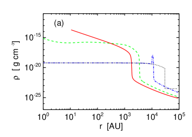
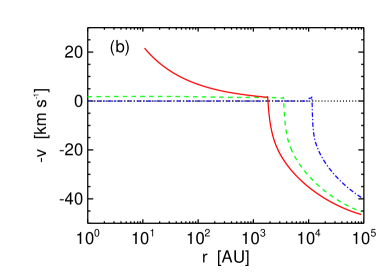
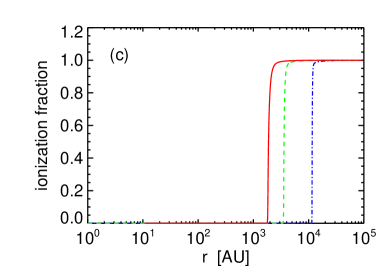
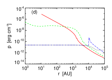
Figure 1: Time evolutions of (a) density profile, (b) velocity profile, (c) ionization fraction and (d) pressure profile in the model with $\xi_{max}=5$ and $d=9$ pc. The dotted lines denote the profiles at $t=0$. The profiles at $t=0.66\times 10^{5}{\mathrm{y}r}$, $t=1.02\times 10^{5}{\mathrm{y}r}$, and $t=1.09\times 10^{5}{\mathrm{y}r}$ are labeled by dash-dotted, dashed, and solid lines, respectively.

To illustrate common features of the time evolution, we describe results in model C with $d=9\ \mathrm{pc}$ listed in Table 1. Fig. 1 shows the time evolution of density, velocity, ionization fraction, and pressure. Initially, the core was in hydrostatic equilibrium with the rarefied warm neutral gas. At $t=0$, UV radiation, whose UV photon flux is $F_{i}$, turned on and illuminated from the outer boundary. The outer layer of the core was ionized by UV radiation. Temperature and pressure at this outer layer increased drastically. The hot ionized gas then expanded outwards, accelerated to $\sim 40\ \mathrm{km\,s^{-1}}$, and drove a shockwave into the core. At $t=1.02\times 10^{5}\ \mathrm{yr}$, the shockwave reached center of the core. The dashed line in Fig.1(a) shows that the core is compressed into a small region of a radius $\sim 3700\ \mathrm{AU}$ at this time. The density becomes $\sim 10^{3}$ times higher than the initial density and the core becomes gravitationally unstable.

The core collapses subsequently. We see from Fig.1 (a) and (b) that density and velocity of the compressed core increase rapidly after $t=1.02\times 10^{5}\ \mathrm{yr}$ due to self-gravity. After the central density exceeds the reference value $\rho_{sink}$, the sink-cell treatment turns on, at which point a protostar forms at the center of the core. At this phase, inner region of the core accretes onto the central protostar, and the ionized outer layer expands outward.

Velocities of the shock front and the ionization front remain nearly constant, on the other hand. Fig. 2 shows locations of the ionization and the shock fronts as functions of time. Velocity of the shock front is a constant value of $\sim 1.37\ \mathrm{km\,s^{-1}}$. Analytic estimation described in section 4.1 shows a similar velocity of $1.18\ \mathrm{km\,s^{-1}}$. For convenience, we define ionization front at the location where the ionization fraction is 0.9. How ionization front is defined in fact hardly affects the results, since, as shown in Fig. 1(c), the transition layer from neutral to ionized gas is very thin. Average velocity of the ionization front is $1.23\ \mathrm{km\,s^{-1}}$, and analytic estimation shows a similar velocity of $1.14\ \mathrm{km\,s^{-1}}$.

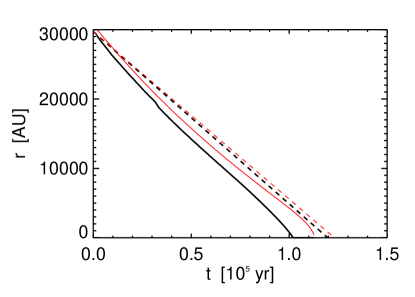
Figure 2: Locations of the ionization front and shock front. The thick (black) and thin (red) solid lines label the position of shock front and ionization front in model C with $d=9\ \mathrm{pc}$, respectively. The thick (black) and thin (red) dashed lines label the analytic estimates described in section 4.1, respectively.

Some fraction of the incident UV photons is absorbed in the layer of the photo-evaporated gas. In this layer, ionized hydrogen atoms recombine with electrons at the rate of $\alpha x^{2}n$ per unit volume per unit time. Some UV photons are used for ionization of these recombined hydrogen atoms. We define Q, the ratio of UV photon flux at the ionization front to the incident UV photon flux, as the photo-evaporation rate of the core. Fig. 3 shows Q as a function of radius. Spitzer (1978) derived an analytic estimation of $Q$ as

$$Q=\frac{2}{1+\sqrt{1+\frac{4\alpha F_{i}r_{IF}}{3c_{i}^{2}}}},$$ (9)

where $r_{IF}$ is the radius of the ionization front. Our numerical results show a slightly larger value than that of the analytic estimation by assumptions. Spitzer (1978) assumed that the photo-evaporated gas expands at the constant sound speed $c_{i}$. As shown in Fig.1(b), however, the photo-evaporated gas accelerated to $\sim 3c_{i}\,(\sim 40\mathrm{k\,ms^{-1}})$ in our simulations due to pressure gradient. This high velocity reduces the density of the photo-evaporated gas. As a result, the recombination rate of hydrogen atoms is smaller than that of the analytic estimate.

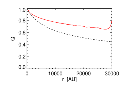
Figure 3: The ratio of UV photon flux at ionization front to incident UV photon flux as a function of radius in the model C with $d=9\ \mathrm{pc}$. The dashed line indicates the analytic estimation which is given by Eq. (9).

3.2 Accretion Rates

As a reference, we simulate the spontaneous collapse of the core without UV radiation. Since the thermal pressure balances the gravitational force in the Bonnor-Ebert sphere, we slightly enhance the density to $\rho=1.05\,\rho_{BE}$, where $\rho_{BE}$ is the density of a marginally stable Bonnor-Ebert sphere ($\xi_{max}=6.45$), to initiate collapse. This core whose mass is 3 $M_{\sun}$ collapses by self-gravity, and the averaged value of accretion rate is $7.4\times 10^{-6}\ \mathrm{M_{\sun}\ yr^{-1}}$.

The RDI indeed increases accretion rates. Fig. 4 shows the accretion rate as a function of time in model C with $d=9\ \mathrm{pc}$. The accretion rates are measured at the radius of 10 AU. The horizontal line indicates the average accretion obtained from the reference model. At $t=1.02\times 10^{5}\ \mathrm{yr}$, the central density reaches the threshold density $\rho_{sink}$, and the sink cell method turns on. The accretion rate increases rapidly afterwards, and lasts for $\sim 10^{4}\mathrm{yr}$.

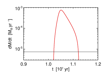
Figure 4: Accretion rate as a function of time in the model C with $d=9\ \mathrm{pc}$. The horizontal line indicates the averaged value of accretion rate in model without UV radiation.

Fig. 5 shows the averaged values of accretion rates as a function of distance from the ionizing star. The accretion rates increase with decreasing distance from the ionizing star, and with the increasing UV photon flux. If the cores are located within 10 $\mathrm{pc}$ from an ionizing star, the accretion rates can go 1-2 orders higher than models without UV radiation.

The accretion rates not only depend on the UV photon fluxes but also on $\xi_{max}$ and $M_{0}$. Cores with larger values of $\xi_{max}$ have smaller radii and higher densities. Shock velocities and densities in post-shock regions are larger in the models with small $\xi_{max}$. Gas of higher density has a shorter free-fall time, and reaches an accretion rate higher in the models with smaller $\xi_{max}$. We will compare this with analytic estimates for better understanding. In the model G, not only small free-fall time but also large mass of compressed core is responsible for high accretion rate.

Figure 5: The averaged accretion rates as functions of distance from the ionizing star. Open diamonds, open squares, open circles label results from the model A, B, and C, respectively. Filled diamonds, filled squares, filled circles label models D, E, and F, respectively. The crosses are for the model G. The horizontal line indicates the averaged accretion rate in the reference model. Dotted line, dash-dotted line and dashed line indicate analytic estimation for models A, B, and C, respectively.

3.3 Final Masses

Photo-evaporation can reduce the actual mass that accretes onto the protostar. In the outer layer, hot ionized gas expands outward at a velocity up to $\sim 40\ \mathrm{km\,s^{-1}}$. Photo-evaporation of gas takes place at $\sqrt{2GM/r}$, except for the case of very small cores. The escape velocity of the Bonnor-Ebert sphere in model C is $\sim 0.42\ \mathrm{km\,s^{-1}}$, for example, is much smaller than that of the photo-evaporated flow. Photo-evaporation prevents large amount of gas from accreting onto the protostar, and final mass of the protostar can be small due to mass loss by photo-evaporation.

Final masses of protostars decrease with decreasing distance from the ionizing star. Fig. 6 shows the final masses of protostars as functions of distance from ionizing star. The mass of a protostar is defined as mass which has entered sink cells, and calculations continue until accretion rates become sufficiently small ($10^{-9}\ \mathrm{M_{\sun}\,yr^{-1}}$). Mass loss due to photo-evaporation at the surface of the core is proportional to the incident UV photon flux and final masses of protostars are smaller near the ionizing star. For an O8V or an O4V star, mass loss due to photo-evaporation varies from several percent to several tenth of percent of the initial core mass. The more massive the ionizing star gets, the smaller the final mass.

The final masses not only depend on the UV photon fluxes but also on the sizes of cores. Fig. 6 shows that mass loss due to photo-evaporation is significant in the model G, in which initial radius of the core is 10 times larger than that in the model C. Larger core has larger photo-evaporation rate and longer time to be exposed to UV radiation because of larger surface area and longer crossing time of shock wave. This is the reason why the core lose large amount of mass in the model G. For the same reason, final masses are small in the models with small $\xi_{max}$.

Figure 6: Ratio of final mass of protostar to initial core mass as a function of distance from ionizing star. The open diamonds, the open squares, the open circles indicate results in the models A, B, and C, respectively. The filled diamonds, the filled squares, the filled circles indicate results in the models D, E, and F, respectively. The crosses indicate results in the model G. The dotted line, the dash-dotted line and the dashed line indicate analytic estimation for model A, B,and C, respectively.

4 Discussion

4.1 Analytic Estimates

In this section, we derive analytic estimates of final mass and accretion rates of protostars under the influence of RDI. For simplicity, we assume that a core has a uniform density $n_{0}$ and a radius $R_{0}$ initially. The core is exposed to UV radiation whose number flux of UV photons is $F_{i}$. Spherical symmetry is assumed.

The final mass of protostar $M_{f}$ is expressed as

$$M_{f}=M_{0}-\int_{0}^{t_{s}}\!4\pi r_{IF}(t)^{2}\dot{m}\,dt,$$ (10)

where $r_{IF}(t)$ is the radius of the ionization front at time $t$, $\dot{m}$ is the mass loss flux at radius $r_{IF}(t)$, and $t_{s}$ is the crossing time of the shockwave. The second term on the right-hand side of Eq. (10) expresses mass loss due to photo-evaporation. We only consider mass loss during the compression phase when the core is compressed into a small region by the shock. After the compression, the core collapses within the free-fall time of the compressed core that is much shorter than $t_{s}$. We need $\dot{m}$, $t_{s}$, and $r_{IF}(t)$ to estimate the final mass of protostars using Eq. (10).

The mass loss flux $\dot{m}$ due to photo-evaporation is expressed as

$$\dot{m}=m_{H}QF_{i}.$$ (11)

where $Q$ is the ratio of UV photon flux which arrives at surface of core to incident UV photon flux $F_{i}$. The UV photons ionize the outer layer of the core, but some fraction gets absorbed in the photo-evaporated flow. As shown in Fig. 3, $Q$ approaches to unity as the ionization front enters the inner region of the core. However, we assume that $Q$ remains constant through the compression phase and calculate the value of $Q$ at the radius $R_{0}$ using Eq. (9).

The shock velocity $u_{s}$ is derived following Bertoldi (1989) to estimate the shock crossing time $t_{s}$. Assuming ram pressure of the flow equals thermal pressure of the post-shock region, we obtain

$$n_{0}u_{s}^{2}=c_{n}^{2}n_{1},$$ (12)

where $n_{0}$ and $n_{1}$ are number densities of the undisturbed region and the post-shock region, respectively. The equation of mass continuity at the ionization front gives

$$QF_{i}=n_{1}u_{IF}^{\prime},$$ (13)

where $u_{IF}^{\prime}$ is the velocity of ionization front in the rest frame of the post-shock region. The ionization front is assumed to be D-critical (cf. Spitzer, 1978), and velocity of the ionization front is given as

$$u_{IF}^{\prime}\simeq\frac{c_{n}^{2}}{2c_{i}}.$$ (14)

Substituting Eq. (14) into Eq. (13) gives

$$2Qc_{i}F_{i}=c_{n}^{2}n_{1}.$$ (15)

Combining Eq. (12) and Eq. (15), we obtain

$$u_{s}=\sqrt{\frac{2c_{i}QF_{i}}{n_{0}}}.$$ (16)

Using Eq. (16), the shock crossing time is expressed as

$$t_{s}=\frac{R_{0}}{\sqrt{\frac{2c_{i}QF_{i}}{n_{0}}}}.$$ (17)

We derive the velocity of ionization front $u_{IF}$ in the rest frame of the undisturbed region to obtain radius of the ionization front $r_{IF}(t)$. Taking into account $n_{1}=\left(\frac{u_{s}}{c_{n}}\right)^{2}n_{0}$ and $n_{0}u_{s}=n_{1}(u_{s}-v_{1})$, we obtain

$$v_{1}=u_{s}-\frac{c_{n}^{2}}{u_{s}},$$ (18)

where $v_{1}$ is velocity of the post-shock region in the rest frame of the undisturbed region. Velocity of the ionization front is

$$u_{IF}=u_{s}-\frac{c_{n}^{2}}{u_{s}}+\frac{c_{n}^{2}}{2c_{i}}.$$ (19)

Using $u_{IF}$, radius of the ionization front is expressed as

$$r_{IF}=R_{0}-u_{IF}t.$$ (20)

The final mass of protostar using Eq. (10) gives

$$M_{f}=M_{0}-4\pi m_{H}QF_{i}\,(R_{0}^{2}t_{s}-R_{0}u_{IF}t_{s}^{2}+\frac{u_{IF}^{2}}{3}t_{s}^{3}).$$ (21)

This equation gives us the analytic estimate of final mass of a protostar influenced by RDI.

The accretion rate, over a free-fall time, is roughly estimated by

$$\dot{M}=\frac{M_{f}}{t_{ff}},$$ (22)

where $t_{ff}=\sqrt{\frac{3\pi}{32\rho_{f}G}}$ is the free-fall time of the compressed core. The core is compressed into a radius of $r_{IF}(t_{s})$ when the shock reaches its center. The density of the compressed core is then given as

$$\rho_{f}=\frac{M_{f}}{\frac{4\pi}{3}r_{IF}(t_{s})^{3}},$$ (23)

and Eq. (22) gives us the analytic estimate of the accretion rate.

4.2 Luminosity

Luminosity of a protostar is mainly produced by accretion, because nuclear burning does not influence much of the luminosity during the protostellar collapse phase. The accretion luminosity $L$ is expressed as

$$L=\frac{GM_{*}\dot{M}}{R_{*}},$$ (24)

where $M_{*}$ is the mass, $\dot{M}$ is the accretion rate, and $R_{*}$ is the radius of the protostar. Enhancement of accretion rates due to RDI has a large effect on the luminosity. Although the accretion rate depends not only on the distance from the ionizing star but also on the $\xi_{max}$ of the Bonnor-Ebert sphere, it is relatively not as sensitive to $\xi_{max}$ compared with the distance. Our results show that for cores located within 10 pc of an ionizing star, the accretion rates becomes 1-2 orders of magnitude higher than those without triggering from the UV radiation.

Enhanced luminosity around bright-rimmed clouds is seen in observations. Sugitani et al. (1989) observed three bright-rimmed globules associated with cold IRAS sources in ¹³CO(J=1-0) emission. They compared the physical parameters with four isolated dark globules and found that the ratios of the luminosity to globule mass, $3-13\ L_{\sun}/M_{\sun}$, are 1-2 orders higher than the values of isolated dark globules, $0.03-0.3\ L_{\sun}/M_{\sun}$, as shown by our calculations. These objects are good candidates influenced by the RDI.

Protostars near H ii regions may spend most of their lifetime in the state of high luminosity. If the duration of high accretion rate is much shorter than the lifetime of the protostar, it is relatively difficult to catch the protostar in its high-luminosity state by observations. In the simulations, the protostellar phase begins from the time when the sink-cell method is turned on and lasts until 99 % of the final mass has accreted within the sink cells. The lifetime of the protostar in model C is $9.1\times 10^{3}\ \mathrm{yr}$ with $d=9\ \mathrm{pc}$. As shown in Fig. 4, the accretion rate is enhanced for a duration of $8.4\times 10^{3}\ \mathrm{yr}$, comparable to the lifetime of the protostar. It is likely that protostars near H ii regions be observed in the state of higher luminosity.

4.3 Comparison with observations

Table 2: Star formation regions of potential triggered origins

Cloud	Spectral type of	Projected distance from	Estimated shock		Evidence of triggered
	main ionizing star	ionizing star	velocity		star formation
molecular pillars in M161	O5V	2 pc	1.3 $\mathrm{k\,ms^{-1}}$		age gradient of YSOs
IC1396N2	O6.5f	11 pc	0.6 $\mathrm{k\,ms^{-1}}$		age gradient of YSOs
SFO11, SFO11NE, SFO11E3	O6V	11 pc	1.4 $\mathrm{k\,ms^{-1}}$		on-going star formation
					near ionization front
Orion bright-rimmed clouds4	O8IIIa or O6:b	-	-		on-going star formation
					near ionization front

^a Ionizing star of B30 and B35.
^b Ionizing star of IC2118, LDN1616, and LDN1634.
References: (1) Fukuda et al. (2002), White et al. (1999), (2) Getman et al. (2007), (3) Thompson et al. (2004), (4) Lee et al. (2005)

Evidences of triggered star formation have been suggested on edges of many H ii regions. Some of the observations in fact favor the scenario of sequential star formation around a massive star. Lee et al. (2005) selected candidates of pre-main sequence stars based on 2MASS colors in the Orion region, and revealed spatial distribution of classical T Tauri stars using their spectroscopic observations. The pre-main sequence stars form between the ionizing star and the bright-rimmed clouds, but not deeply inside the cloud. The youngest stars are found near the cloud surfaces, forming an apparent age gradient. As the H ii region expands, it might be able to trigger star formation sequentially from near to far. Several of such examples are summarized in Table 2.

RDI may contribute to the triggering mechanism around a massive star. Lee et al. (2005) found that only bright-rimmed clouds with strong IRAS 100 $\mu m$ and H$\alpha$ emission show signs of ongoing star formation. This suggests that star formation may have been triggered by strong compression from the ionization shock, because these emissions are tracers of dense gas and ionization. Small-scale age gradients of YSOs near the ionization fronts are seen in some molecular clouds. Fukuda et al. (2002) observed heads of molecular pillars $\Pi_{1}$ and $\Pi_{2}$ in the Eagle Nebula (M16). They found that protostars and starless cores are ordered in age sequences. The more evolved objects are closer to the cloud heads (and the ionizing star) and the younger objects are farther from the exciting star. Similar age gradients are also seen in bright-rimmed clouds (Sugitani et al., 1995) and cometary globule IC1396N (Getman et al., 2007). These age gradients near ionization front seem to suggest that star formation may be sequentially triggered by ionization shocks.

Stars formed facing the H ii regions appear to be more luminous. Yamaguchi et al. (1999) carried out ${}^{13}\mathrm{CO(J=1-0)}$ observations toward 23 southern H ii regions and identified 95 molecular clouds associated with H ii regions. They found that IRAS point sources tend to be more luminous on the side facing an H ii region. Their result is consistent with enhanced luminosity as a result of the RDI.

Shock speeds derived from observations are similar. White et al. (1999) and Thompson et al. (2004) derived shock velocities from pressure in pre- and post-shock regions. Getman et al. (2007) derived shock velocity from the age gradients of YSOs. Their estimated values of a few $\mathrm{km\,s^{-1}}$ are consistent with our results. For example, Thompson et al. (2004) estimated that shock velocity in bright-rimmed cloud SFO11 is $\sim 1.4\ \mathrm{km\,s^{-1}}$. SFO11 is illuminated by an O6V star whose projected distance is 11 pc. These conditions are close to those in model C with $d=9$, whose ionizing star is an O8V star. As described in section 3.1, the averaged shock velocity is $\sim 1.37\ \mathrm{km\,s^{-1}}$ in this model.

Lee & Chen (2006) found that classical T Tauri stars exist near the surfaces of bright-rimmed clouds and intermediate mass stars exist relatively inside clouds. One possible difference of stellar mass may be density or mass in the parent cores. Photo-evaporation may reduce the mass that would otherwise accrete onto the stars. In our simulations a few percent to several tenth percent of initial mass may be lost by photo-evaporation. Mass of young stars may be smaller near the surface of bright-rimmed clouds compared with inner regions.

5 Conclusions

We simulate the evolution of cores exposed to strong UV radiation around the H ii regions. We investigate possible effects of the radiation-driven implosion on the accretion luminosity of forming protostars. We also developed analytic estimates of accretion rates and final masses of protostars, which are compared with the numerical results.

The main findings are:

1. Radiation-driven implosion can compress the cores and decrease the free-fall time.

2. The accretion rates are positively influenced by on the incident UV photon flux.

3. Photo-evaporation of the parent cores may decrease the final masses of protostars. However, mass loss due to photo-evaporation does not affect significantly the accretion luminosity.

4. Final mass of a protostar depends mainly on the size of the parent core and incident UV photon flux. Final mass of a protostar decreases with the increase of UV photon flux. Dense compact cores, on the other hand, are hardly affected by mass loss due to RDI.

5. The RDI increases luminosity of protostars by orders of magnitude than spontaneous star formations without RDI.