Velocity distribution of collapsing starless cores, L694-2 and L1197

Abstract

In an attempt to understand the dynamics of collapsing starless cores, we have conducted a detailed investigation of the velocity fields of two collapsing cores, L694-2 and L1197, with high spatial resolution HCN J = 1-0 maps and Monte Carlo radiative transfer calculation. It is found that infall motion is most active in the middle and outer layers outside the central density-flat region, while both the central and outermost parts of the cores are static or exhibit slower motion. Their peak velocities are 0.28 km s^-1 for L694-2 and 0.20 km s^-1 for L1197, which could not be found in simple models. These velocity fields are roughly consistent with the gravitational collapse models of the isothermal core; however, the velocity gradients inside the peak velocity position are steeper than those of the models. Our results also show that the density distributions are $\sim r^{-2.5}$ and $\sim r^{-1.5}$ in the outer part for L694-2 and L1197, respectively. HCN abundance relative to H₂ is spatially almost constant in L694-2 with a value of $7\times 10^{-9}$, while for L1197, it shows a slight inward increase from $1.7\times 10^{-9}$ to $3.5\times 10^{-9}$.

1 Introduction

Starless cores that are on the verge of or undergoing gravitational collapse provide important information on the initial stage of star formation. In order to understand the dynamics of such starless cores, it is necessary to obtain information on at least density, temperature, and velocity distributions. The density and temperature have been determined by submillimeter/NIR and NH₃ observation with a certain degree of accuracy (Evans et al., 2001; Kandori et al., 2005; Tafalla et al., 2004).

However, the velocity field has not yet been elucidated. The observations of starless cores in the molecular lines of CS, $\rm{DCO^{+}}$, and $\rm{N_{2}H^{+}}$ (Lee et al., 1999, 2001, 2004) show that the inward motion is extended to $0.2-0.3$ pc with a speed of $0.05-0.09$ km s^-1, which is derived using a two-layer model (Myers et al., 1996). The analysis of the CS J = 3-2 and J = 2-1 lines with the same model for several cores such as L183, L1521F, L1689B, L1544, and L694-2, suggests that the infall speed appears to increase toward the center (Lee et al., 2004). Since the two layer model is rather simple, the derived velocity may be an average value along the line of sight and its variation with depth should be considered with caution. Moreover, it should be noted that in general, CS is significantly depleted in the central regions of starless cores (Tafalla et al., 2002, 2004). On the other hands, by applying an improved version of the two layer model (De Vries & Myers, 2005) to the interferometric observations in $\rm{N_{2}H^{+}}$, Williams et al. (2006) found that the infall velocity increases toward the emission peak for L694-2 and L1544 . This transition might trace the deep central region of the core because the emission of $\rm{N_{2}H^{+}}$ primarily comes from the central part due to its low optical depth and centrally condensed matter distribution (Tafalla et al., 2006). Therefore, it is highly likely that these independent observations do not trace the entire range of the velocity fields in the collapsing cores. Similar shortcomings are evident in Tafalla et al. (2002), Keto et al. (2004), and Swift et al. (2006), although they have assumed that the infall speed varies monotonically with the radial distance and have performed more sophisticated radiative transfer calculations.

In order to derive a reliable velocity field, by overcoming these problems, we selected HCN J = 1-0 hyperfine lines as a probe and observed several candidates of collapsing cores. Then, we performed radiative transfer calculations by considering different types of velocity fields. An advantage of using the HCN J = 1-0 lines is that three hyperfine lines are well separated and they cover a wide range (a factor of 5) of the optical depth. In addition, a direct comparison between the integrated intensity map of HCN and that of the $\rm{N_{2}H^{+}}$ reveals that HCN is not depleted significantly (Sohn et al., 2004). For radiative transfer analyses, we used the one-dimensional Monte Carlo code by considering the line overlap effect due to the hyperfine splitting of HCN energy levels (Bernes, 1979; González-Alfonso & Cernicharo, 1993; Park et al., 1999). Therefore, the capability of this code is almost the same as that of code used by Tafalla et al. (2002), Keto et al. (2004), and Swift et al. (2006). The only difference is that we explored more complicated velocity fields, by relaxing the condition of the monotonic increase or decrease of velocity field, which is an implicit assumption of the previous studies.

2 Data

We analyzed two round-shaped collapsing starless cores, L694-2 and L1197, located at $\alpha_{2000}=19^{h}41^{m}04.^{s}5$, $\delta_{2000}=10^{\circ}57^{\prime}02.^{\prime\prime}0$ and $\alpha_{2000}=22^{h}37^{m}02.^{s}3$, $\delta_{2000}=58^{\circ}57^{\prime}20.^{\prime\prime}6$, respectively. The observations were performed in September 2003 by using the IRAM 30 m at a spacing of 11^′′ (Sohn et al., 2004). The beam size of the telescope was $\rm{FWHM}=28^{\prime\prime}$ for the HCN J = 1-0 and the velocity resolution of the backend was 0.033 km s^-1. Data were converted to the T_mb scale using a main beam efficiency of 0.82. We set the frequency of the three HCN J = 1-0 hyperfine lines according to the Cologne Database for Molecular Spectroscopy (M$\rm{\ddot{u}}$ller et al., 2005) as follows: 88.6304157 GHz for F = 0-1, 88.6318473 GHz for F = 2-1, and 88.6339360 GHz for F = 1-1.

In order to perform a comparison with the one-dimensional radiative transfer calculations, we assumed that two cores are spherically symmetric. It is justified by the spherically symmetric density distribution from the observation of dust extinction and emission for L694-2 (Harvey et al., 2003a, b). The HCN J = 1-0 line profiles are distributed concentrically and they all exhibit blue asymmetry for L694-2. This is the case for L1197 except for red asymmetry in south-west region occupying only $\leq$ 10% of the observed area, which has a negligible contribution to the analysis. The observations will be described in detail in a separate paper (Sohn et al. , in preparation). The observed spectra were azimuthally averaged at concentric radial annuli with a step of 10^′′. We set the centers of the cores to the peak intensity positions of $\rm{N_{2}H^{+}}$, which are (0^′′, 0^′′) for L694-2 and (0^′′, 11^′′) for L1197 relative to the map centers mentioned above. Since the spectra were at rectangular grid points, they were weighted by a factor of $exp(-(d/14^{\prime\prime})^{2})$, where $d$ is the distance in arcseconds between the radial distance of the grid point and the specified radius and 14^′′ is one half width of telescope beam. The resulting spectra are shown in Fig. 1 and will be used as templates for the comparison with synthesized line profiles.

3 Model of core

We synthesized line profiles by using the Monte Carlo radiative transfer model and compared them with the observed ones in order to derive the model parameters that best explain the observations. We adopted distances of 250pc and 400 pc to L694-2 and L1197, respectively (Lee et al., 2001). Velocities relative to the local standard of rest were selected as 9.61 km s^-1 and $-3.16$ km s^-1 for L694-2 and L1197, respectively. The model cores with a radius of 0.15 pc for both L694-2 and L1197 were composed of 30 concentric shells at regular intervals. Additionally, these cores were surrounded by an envelope with an adjustable radius (see below). We used $10^{6}$ model photons for the Monte Carlo code.

The kinetic temperature was assumed to be spatially constant at 10K, on the basis of the values derived for L1498 and L1517B (Tafalla et al., 2004). For the density distribution, we used the following form adopted by Tafalla et al. (2004),

$$n(r)={n_{c}\over 1+(r/r_{o})^{\alpha}}\ \ ,$$ (1)

where $n_{c}$ is the central density, $r_{o}$ is the radius of the inner flat region, and $\alpha$ is the asymptotic power index. In dynamic models, $r_{o}$ decreases with an increase in the central density (Foster & Chevaler, 1993; Ciolek & Basu, 2000). To consider this effect, we defined $r_{o}$ such that it depended on $n_{c}$,

$$r_{o}\equiv 2.25R_{o}\ \ ,$$ (2)

$$R_{o}=a/\sqrt{4\pi G\mu m_{H}n_{c}}\ \ ,$$ (3)

where $R_{o}$ is the scale radius of the Bonnor-Ebert sphere, $a$ is the sound speed, $\mu$ (= 2.33) is the mean molecular weight, and $m_{H}$ is the hydrogen mass. If $\alpha$ is 2.5 in equation (1), it represents approximately the density distribution of the Bonnor-Ebert sphere (Tafalla et al., 2004). In our model, we tested two cases of sound speed, $a$ = 0.2 and 0.3 km s^-1, and finally adopted the latter.

Since the integrated intensity map of the thinnest HCN J = 1-0, F = 0-1 line is similar to that of the N₂H⁺ J = 1-0 line, it appears that HCN is not significantly depleted for these two cores at least (Sohn et al., 2004). In order to take into account any minor depletion or enhancement of HCN, we assumed the HCN abundance variation of $X(r)$ $=$ $X_{o}[n(r)/n_{o}]^{\beta}$, where $\beta$ is the power index and $n_{o}$ and $X_{o}$ are the density and HCN abundance relative to H₂ near the boundary, respectively. $n_{o}$ were fixed lastly as $5\times 10^{3}$ cm^-3 for L694-2 and $1\times 10^{4}$ cm^-3 for L1197, respectively.

The line profiles are most sensitive to the infall velocity field. We characterized the velocity field as a $\Lambda$-shaped field. (The reason why we adopted this shape will be discussed in next section.) The innermost region within $R_{i}$ is static, and the infall velocity increases with a linear function of the radial distance toward the peak velocity position ($R_{m}$) with a maximum magnitude of $V_{m}$, and then linearly decreases to the outermost layer. We fixed the size of the outermost layer and its velocity to $0.13{\rm pc}\leq r\leq 0.15{\rm pc}$ and a constant, respectively. In fact, the size of the outermost layer is determined on the basis of the first several trials. The velocity of the outermost layer can be directly derived from the line profile. The fitting procedure will be described in detail in next section.

In summary, we have seven free parameters in total : $n_{c}$ and $\alpha$ for density, $X_{o}$ and $\beta$ for abundance, and $R_{i}$, $R_{m}$, and $V_{m}$ for velocity. We made reference to the values of previous studies for density and abundance (Harvey et al., 2003a, b; González-Alfonso & Cernicharo, 1993).

Besides these, a few auxiliary parameters were necessary to fit the line profiles. The e-folding widths of the absorption coefficient profile in the inner static region were specified as 0.15 km s^-1 and 0.13 km s^-1 for L694-2 and L1197, respectively; they are larger than the pure thermal width by a factor of $\sim 2$. In the other layers, these widths were automatically adjusted such that the line widths of the model spectra closely resembled the observed ones. To explain the hyperfine anomalies of HCN, an envelope with larger microturbulence width and lower density must be introduced (González-Alfonso & Cernicharo, 1993). The diffuse and turbulent molecular clouds surrounding the cores traced by CO may be considered as the envelope (Tafalla et al., 2006). We selected the microturbulence width of 0.5 km s^-1 and the abundance of $5\times 10^{-9}$, which were the same for both cores. The density was set to $10^{3}$ cm^-3 for L694-2 and $3\times 10^{3}$ cm^-3 for L1197. Then, we varied the size of the envelope to adjust the relative intensity ratio among the hyperfine lines. It is not necessary for the envelope parameters to be unique since various combinations of the density, abundance, and size are acceptable if the optical depth is almost the same and the excitation temperature is sufficiently low and close to 2.7 K. It should be noted that the envelope is introduced to account for only the intensity ratio among the hyperfine lines.

The line profiles produced by this method were convolved with the telescope beam for a direct comparison with the observations. The difference between the model line profile and the observed one was evaluated by $\chi^{2}$ (Zhou et al., 1993). We considered all channels of three hyperfine transitions on 5 positions, in the velocity range from $-0.7$ km s^-1 to $0.7$ km s^-1.

4 Results

In the first phase, we adjusted the density distribution and constant HCN abundance without infall motion so that the intensities of F = 0-1 at all locations are similar to those observed. Further, we attempted to fit the line profiles with the infall velocity fields of the constant or monotonically increasing/decreasing function of the radius and found that they cannot reproduce the observed spectra. The infall velocities at every grid points were then varied by trial and error. It was immediately evident that the infall motion is dominant in the middle and outer layers and other parts of the cores are rather static or exhibit a small amount of motion. Therefore, we approximated the velocity field with the $\Lambda$-shaped one.

The $\Lambda$-shaped velocity field could be qualitatively understood by inspecting the characteristic features of the observed line profiles shown in Fig. 1 as follows. On the basis of the fact that the position of the self-absorption dip in the thickest F = 2-1 line indicates the velocity at the outermost part, we can estimate the infall velocity in that region. These infall velocities for L694-2 and L1197 are $\approx 0.0$ and $\approx 0.1$ km s^-1, respectively. On the other hand, the velocity in a region close to the central part can be derived from the line width of an optically thin N₂H⁺ line, since it is not depleted significantly and, therefore, its emission mainly originates from the central part in which the density is the highest. From Lee et al. (1999), the FWHM of L694-2 and L1197 are found to be 0.27 km s^-1 and 0.28 km s^-1, respectively. These values can be used to derive the contribution of non-thermal motion after removing the thermal width. If this motion is attributed to the systematic inward motion, the maximum infall velocity will be 0.12 km s^-1 for both L694-2 and L1197. Since cores with a pure thermal line width are extremely rare, the systematic motion will be even smaller. The line shape also provides information on the velocity field in the middle layer. The increasing rate of the brightness from the absorption dip to red part is considerably slower than to blue part, particularly for L694-2, thereby resulting in a weaker red peak. This suggests that the region of $\tau_{\nu}=1$ remains close to the surface layer in the red part, implying that the infall velocity increases steeply toward the deeper layer. Then, it must decrease again toward the center to satisfy the constraints of the N₂H⁺ lines.

In the second phase, in order to derive the velocity field in a more systematic manner, we reduced the number of parameters describing the velocity field to three, $R_{i}$, $R_{m}$, and $V_{m}$ as mentioned in the previous section. First, we adjusted the parameters of the velocity field, while fixing the other density and abundance parameters. Thereafter, the density parameters were modified followed by the abundance parameters, while the other parameters were unchanged. We repeated this process a few times.

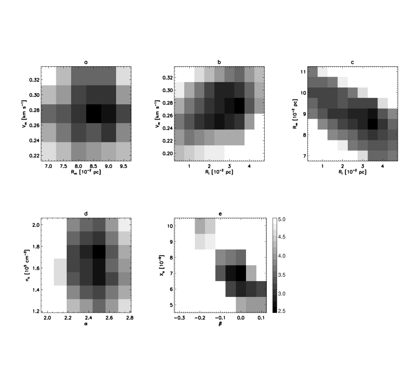
Figure 3: Distribution of $\chi^{2}$ around the best fit solution with $\chi^{2}$ of 2.7 as a function of model parameters for L694-2 (see text for the best fit model parameters). Panels a, b, and c are about velocity field, and d and e are about density and abundance distribution, respectively.

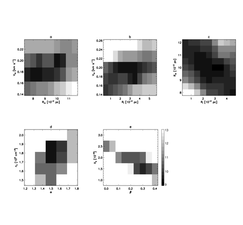
Figure 4: Distribution of $\chi^{2}$ around the best fit solution with $\chi^{2}$ of 9.2 as a function of model parameters for L1197. Others are the same as in Fig. 3.

The spectra of the best fit models are displayed in Fig. 1, where one can note that almost all the details are reproduced, particularly for L694-2. The density and velocity distribution of the models are shown in Fig. 2. The minimum $\chi^{2}$’s are estimated to be 2.7 and 9.2 for L694-2 and L1197, respectively. The distributions of the $\chi^{2}$ around the best fit model are displayed in Fig. 3 and Fig. 4. As expected, the abundance parameters are not completely independent, since both are related to the column density of HCN. There seems to be (anti-)correlations among the velocity parameters, too.

To summarize, the infall velocity begins to increase from 0 near the $R_{i}=0.035$ pc for both the cores, and reaches the maximum infall velocity of $V_{m}=0.28$ km s^-1 at $R_{m}=0.085$ pc for L694-2 and $V_{m}=0.20$ km s^-1 at $R_{m}=0.10$ pc for L1197 as shown in Fig. 2. The central density and power index of L694-2 are around $n_{c}=1.75\times 10^{5}$ cm^-3 and $\alpha=2.5$, while those of L1197 are $n_{c}=1.75\times 10^{5}$  cm^-3 and $\alpha=1.5$, respectively. Our result of L694-2 is similar to that derived from the near-infrared extinction and dust emission maps (Harvey et al., 2003a, b). The abundance is uniform with $7\times 10^{-9}$ for L694-2 ($\beta\approx 0.0$), while it increases slightly toward the center for L1197 ($\beta\approx 0.3$) from $1.7\times 10^{-9}$ to $3.5\times 10^{-9}$.

5 Discussion

Since we optimized several parameters cyclically, it is uncertain whether they are a set of best fit parameters. This may be true because we did not explore sufficient parameter spaces. However, since our optimization is based on the qualitative understanding of line profile formation, it is unlikely that a quite different solution will exists. The degree of coincidence of the synthesized and the observed line profiles also supports this argument, as shown in Fig. 1. Although a new solution may be derived, but characteristic features such as the $\Lambda$-shaped velocity field will remain unchanged.

The fact that the velocity distribution is concentrated in the middle and outer layers is attributed to the selection of HCN hyperfine lines that can probe a wide range of core interiors and to the relaxation of the condition of a constant or monotonic decrease/increase in the velocity field. Our model naturally explains the “extended inward motion” observed for several starless cores since the infall motion is dominant in the middle and outer layers. The size of the infalling layer is $\approx 2R_{m}\sim 0.2$ pc, which is consistent with the observations (Myers, 2005). The extended inward motion probed by CS toward L1544 and L1551 appears to be exceptional in that it extends over very wide area. This may be due to other types of motion (Swift et al., 2006).

The velocity field that we found does not contradict the observation of Williams et al. (2006), in which increasing inward motion toward the center in the central 30^′′ region of L694-2 is derived. For this, they used the optically thin N₂H⁺ line to probe the infall velocity of $<~{}0.1$  km s^-1 and therefore the more dominant motion in the middle and outer layers has been missed. In our case, we assumed that the velocity in the central region is zero in order to reduce the number of parameters. In fact, we have tested several sets of models whose velocity fields have non-zero values in the deeper part, and have found that the velocity of $<0.1$  km s^-1 is acceptable.

The distribution of the infall motion of our model is similar to that of the ambipolar diffusion model and isothermal core collapse model (Ciolek & Basu, 2000; Foster & Chevaler, 1993) in the sense that the models also have the $\Lambda$-shaped velocity field and their infall velocity peaks lie just outside the central density-flat region. However, the velocity gradient of our model inside the velocity peak position is steeper than that predicted by the dynamic models. We can observe such a sudden decrease in the infall motion in the deeper layer in the so-called first collapse phase of the model used in Masunaga et al. (1998). However, this occurs when the central part is very dense and opaque at an evolutionary stage later than that of our sample. Some mechanisms resisting against gravity such as rotation may work; however, they are easily excluded since rotation is very slow (Williams et al., 2006). An oscillation of starless cores around equilibrium may be able to explain this, as shown in Keto & Field (2005), where pressure wave reflected from center combined with inward motion due to perturbation from outside results in the steep velocity gradient in the middle. However the magnitude of the motion is much less than sound speed. In the case of L694-2 and L1197, the inward motion is similar to or greater than the sound speed, suggesting that they are undergoing dynamical collapse. The mechanism of a steeper pressure gradient should be sought, but it is inappropriate to describe it in greater detail at this stage.

The motion of the ambipolar diffusion model (Ciolek & Basu, 2000) is very slow and therefore it cannot be used to explain the velocity field derived in this study. This is because the model of Ciolek & Basu (2000) is developed for L1544 when the infall velocity of this core was known to be less than 0.1 km s^-1. If the magnetic field is reduced to explain the infall motion of the cores with ambipolar diffusion, the model will be supercritical and reduced to the usual isothermal collapse model.

6 Conclusion

By combining high spatial resolution HCN observation toward L694-2 and L1197 with the Monte Carlo radiative transfer calculation, we have found that the infall velocity is most dominant in the middle and outer layers of the cores and the infall velocity can be as large as 0.3 km s^-1. The most important feature of our study is that the velocity field is determined with such accuracy and fidelity that it is possible to compare dynamics and observations for the first time. An extensive investigation of the velocity distribution in collapsing starless cores is in progress (Sohn et al., in preparation). The result will clarify the dynamic status of starless cores in greater detail.

Figure 1: The comparison of spectra from the best fit model (line) and those from the observation (histogram) for L694-2 (left) and L1197 (right) as a function of projected radial distance, which is noted in the rightmost panels. Observed spectra are shifted so that their LSR velocity is zero.

Figure 2: The density and infall velocity distributions of the best fit model for L694-2 (left) and L1197 (right).

References

- Bernes (1979) Bernes, C., 1979, A&A, 73, 67
- Ciolek & Basu (2000) Ciolek, G.E., Basu, S., 2000, ApJ, 529, 925
- De Vries & Myers (2005) De Vries, C.H., Myers, P.C., 2005, ApJ, 620,800
- Evans et al. (2001) Evans, N.J.,II., Rawlings, J.M.C., Shirley, Y.L., Mundy, L.G., 2001, ApJ, 557, 193
- Foster & Chevaler (1993) Foster, P.N., Chevalier, R.A., 1993, ApJ, 416, 303
- González-Alfonso & Cernicharo (1993) Gonzá lez-Alfonso, E., Cernicharo, J., 1993, A&A, 279, 506
- Harvey et al. (2003a) Harvey, D.W.A., Wilner, D.J., Myers, P.C., Tafalla, M., 2003a, ApJ, 597, 424
- Harvey et al. (2003b) Harvey, D.W.A., Wilner, D.J., Lada, C.J., Myers, P.C., Alves, J.F., 2003b, ApJ, 598, 1112
- Kandori et al. (2005) Kandori, R., et al. , 2005, AJ, 130, 2166
- Keto & Field (2005) Keto, E., Field, G., 2005, ApJ, 635, 1151
- Keto et al. (2004) Keto, E., Rybicki, G.B., Bergin, A., Plume, R., 2004, ApJ, 613, 355
- Lee et al. (1999) Lee, C.W., Myers, P.C., Tafalla, M., 1999, ApJ, 526, 788
- Lee et al. (2001) Lee, C.W., Myers, P.C., Tafalla, M., 2001, ApJS, 136, 703
- Lee et al. (2004) Lee, C.W., Myers, P.C., Plume, R., 2004, ApJS, 153, 523
- Masunaga et al. (1998) Masunaga, H., Miyama, S.M., Inutsuka, S., 1998, ApJ, 495, 346
- Mller et al. (2005) Mller, H.S.P., Schlder, F., Stutzki, J., Winnevisser, G., 2005, J.Mol.Struct. 742, 215
- Myers (2005) Myers, P.C., 2005, ApJ, 623, 280
- Myers et al. (1996) Myers, P.C., Mardones, D., Tafalla, M., Williams, J.P., Wilner, D.J., 1996, ApJL, 465, 133
- Park et al. (1999) Park, Y.-S., Kim, J., Minh, Y. C., 1999, ApJ, 520, 223
- Sohn et al. (2004) Sohn, J., Lee, C.W., Lee, H.M., Park, Y.-S. Myers, P.C., Lee, Y., Tafalla, M., 2004, JKAS, 37, 261
- Swift et al. (2006) Swift, J., Welch, W., Francesco, J.D., Stojimirovíc, I., 2006, ApJ, 637, 392
- Tafalla et al. (2002) Tafalla, M., Myers, P.C., Caselli, P., Walmsley, C.M., Comito, C., 2002, ApJ, 569, 815
- Tafalla et al. (2004) Tafalla, M., Myers, P.C., Caselli, P., Walmsley, C.M., 2004, A&A, 416, 191
- Tafalla et al. (2006) Tafalla, M., Santiango-Garía, J., Myerys, P.C., Caselli, P., Walmsley, C.M., Crapsi, A., 2006, A&A, 455, 577
- Ward-Thompson et al. (1994) Ward-Thompson, D., Scott, P.F., Hills, R.E., André, P., 1994, MNRAS, 268, 276
- Williams et al. (2006) Williams, J. P., Lee, C.W., Myers, P.C., 2006, ApJ, 636, 952
- Zhou et al. (1993) Zhou, S., Evans, N.J.II., Kmpc, C., Walmsley, C.M., 1993, ApJ, 404, 232