An Elementary Introduction to the JWKB Approximation

Abstract

Asymptotic expansion of the second-order linear ordinary differential equation $\Psi^{\prime\prime}+k^{2}f(z)\Psi=0$, in which the real constant $k$ is large and $f={\rm O}(1)$, can be carried out in the manner of Liouville and Green provided $f$ does not vanish. If $f$ does vanish, however, at $z_{0}$ say, then Liouville-Green expansions can be carried out either side of the turning point $z=z_{0}$, but it is then necessary to ascertain how to connect them. This was first accomplished by Jeffreys, by a comparison of the differential equation with Airy’s equation. Soon afterwards, the situation was found to arise in quantum mechanics, and was discussed by Brillouin, Wentzel and Kramers, after whom the method was initially named. It arises throughout classical physics too, and is encountered frequently when studying waves propagating in stars. This brief introduction is aimed at clarifying the principles behind the method, and is illustrated by considering the resonant acoustic-gravity oscillations (normal modes) of a spherical star.

1 Introduction

It is common, and often apparently most straightforward, to approach problems in macroscopic stellar physics by solving the governing equations numerically. However, simple analytical techniques are often more revealing. For the latter it is usually necessary to idealize the situation in hand, sometimes grossly so, to render  the equations tractable. The outcome can reveal the phenomenon under study in a very different light from that provided by specific numerical examples. In particular, because in some respects analytical results are more general, appreciation of their structure can guide one more easily towards greater understanding. Even viewed merely as a diagnostic tool, that understanding, and sometimes just the analytical solutions themselves,  have proved to be useful in the past simply for finding errors in numerical computations, both before and after publication. Numerical and analytical investigations are complementary, and each would be much poorer without the other.

This is the first of a short series of invited articles intended to illucidate some of the analytical techniques that are used in macroscopic stellar physics. It discusses one of the most useful techniques for studying the wave-like solutions of ordinary linear differential equations of second order: namely, the so-called Liouville-Green expansion combined with the method of Jeffreys for connecting solutions across turning points, more commonly known as the WKB approximation. The method is presented and, I hope, made plausible, giving a slight flavour of the background arguments without resorting to mathematical proof, with the aim of guiding those not already conversant with the method towards its proper use.

2 The Liouville-Green expansion

In modern times, the term WKB approximation has commonly been assigned to what is more properly regarded as the leading term in the Carlini–Liouville–Green (LG) expansion of solutions of the second-order ordinary linear differential equation

$$\frac{{\rm d}^{2}\Psi}{{\rm d}z^{2}}+k^{2}f(z)\Psi=0~{},$$ (1)

in which $k$ is real (positive) and large, and $f={\rm O}(1)$ is slowly varying, in the sense that $k\gg|H^{-1}_{f}|\equiv|-{\rm d}\ln f/{\rm d}z|~{}$. Such equations arise throughout classical physics in describing waves, and asymptotic approximations to their solutions appear to have been considered first by Carlini (1817), actually in a study of a problem in celestial mechanics, and subsequently by Green (1837) and by Liouville (1837).

One of the simplest physical examples is that of small-amplitude adiabatic acoustic waves in an otherwise homobaric fluid, whose linearized governing equations are

$$\rho_{0}\frac{\partial^{2}\mbox{\boldmath$\xi$}}{\partial t^{2}}=-\nabla p^{\prime}~{},$$ (2)

$$p^{\prime}=\delta p=c^{2}\delta\rho=c^{2}\left(\rho^{\prime}+\mbox{\boldmath$\xi$}.\nabla\rho_{0}\right)=-\rho_{0}c^{2}\rm{div}\,\mbox{\boldmath$\xi$}~{},$$ (3)

where $p=p_{0}+p^{\prime}$ is pressure, $\rho=\rho_{0}+\rho^{\prime}$ is density and $\xi$ is displacement, the zero denoting equilibrium value, the prime, Eulerian perturbation, and $\delta$ denoting Lagrangian perturbation. The square of the sound speed in the unperturbed fluid is given by $c^{2}=\gamma_{1}p_{0}/\rho_{0}$, where $\gamma_{1}$ is the first adiabatic exponent. The unperturbed pressure $p_{0}$ is constant, and in this simple case $\rho_{0}$ and $c^{2}$ are considered to vary with only a single Cartesian coordinate $z$, and not with time, $t$. The divergence of equation (2) may be combined with equations (2) and (3) to yield the equation

$$\nabla^{2}\delta p+H_{\rho}^{-1}\mbox{\boldmath$n$}.\nabla\delta p-{1\over c^{2}}{\partial^{2}\delta p\over\partial t^{2}}=0~{},$$ (4)

where $H_{\rho}^{-1}\mbox{\boldmath$n$}=-\nabla\rm{ln}\rho_{0}$ defines the density scaleheight $H_{\rho}$, and $n$ is a unit vector in the $z$ direction. In the special case in which the disturbance $\delta p$ varies only in the $z$ direction, equation (4) reduces to the Klein-Gordon equation

$${\partial^{2}\chi\over\partial t^{2}}+\omega^{2}_{\rm c}\chi=c^{2}{\partial^{2}\chi\over\partial z^{2}}~{},$$ (5)

where $\chi=\rho^{-{1\over 2}}_{0}\delta p$ and

$$\omega^{2}_{\rm c}(z)={c^{2}\over 4H^{2}_{\rho}}\left(1-2{{\rm{d}}H_{\rho}\over{\rm{d}}z}\right)~{}.$$ (6)

Because $\rho_{0}$ and $c^{2}$ are constant in time and are independent of the co-ordinates perpendicular to $n$, equation (4) admits oscillatory solutions with frequency $\omega$ of the form $\delta p(\mbox{\boldmath$x$},t)=\Re\left[\rho^{1\over 2}_{0}\Psi(z)e^{i\left(\mbox{\boldmath$k$}_{\perp}.\mbox{\boldmath$x$}-\omega t\right)}\right]$, where $\Re$ denotes real part and $\Psi$ satisfies

$$\frac{{\rm d}^{2}\Psi}{{\rm d}z^{2}}+\left(\frac{\omega^{2}-\omega^{2}_{\rm c}}{c^{2}}-k_{\perp}^{2}\right)\Psi=0~{},$$ (7)

in which $k_{\perp}=\left|\mbox{\boldmath$k$}_{\perp}\right|$, where $\mbox{\boldmath$k$}_{\perp}$ is a constant wavenumber component perpendicular to $n$. Equation (7) is essentially of the form of equation (1), provided that $\omega$ is high enough.

If $\rho_{0}$ and $c$ were actually constant, $\omega_{\rm c}$ would vanish and equation (7) would admit solutions $\Psi=\Psi_{0}e^{\pm ik_{\parallel}z}$, where $\Psi_{0}$ is a constant amplitude and $k_{\parallel}=\sqrt{\omega^{2}/c^{2}-k^{2}_{\perp}}$. This represents a wave travelling with speed $v_{\phi}:=\omega/\left|\mbox{\boldmath$k$}\right|=c$ in the direction $\mbox{\boldmath$k$}=\left(\mbox{\boldmath$k$}_{\perp},\pm k_{\parallel}\right)$, provided that $k_{\parallel}$ is real, because the phase $\tilde{\phi}=\mbox{\boldmath$k.x$}-\omega t$ is invariant in a frame of reference moving in the direction of $k$ with speed $v_{\phi}$, namely with $\mbox{\boldmath$x$}=\mbox{\boldmath$x$}_{0}+v_{\phi}t\hat{\mbox{\boldmath$k$}}$, where $\hat{\mbox{\boldmath$k$}}=\left|\mbox{\boldmath$k$}\right|^{-1}\mbox{\boldmath$k$}$. The quantity $v_{\phi}$ is called the phase speed.

This solution motivates the LG expansion. Suppose first that $f>0$ in equation (1). If $c^{2}$ and $\omega_{\rm c}^{2}$ in equation (7) vary
slowly with $z$ one can write $\left(\omega^{2}-\omega^{2}_{\rm c}\right)/c^{2}-k^{2}_{\perp}=k^{2}\kappa^{2}(z)$, where $k$ is constant and $\kappa=f^{1/2}$ is a function whose magnitude is of order unity and whose scaleheight $H_{\kappa}$ is much greater in magnitude than $k^{-1}$. In other words, the equilibrium, background, state varies only little over the characteristic lengthscale $k^{-1}$ of variation of the wave. It is only under such circumstances that the concept of a wave is readily interpreted.

Thus, one poses a wave-like solution to equation (7) by setting

$$\Psi=\Psi_{0}(z)e^{i\tilde{\phi}(z,t)}=\Psi_{0}(z)e^{i(k\psi(z)-\omega t)}~{},$$ (8)

regarding $k$ as a large parameter. It is usual then to expand $\psi$ in inverse powers of $k$; here I shall afford myself the flexibility of expanding both $\psi$ and $\Psi_{0}$:

$$\psi = \psi_{0}+k^{-1}\psi_{1}+k^{-2}\psi_{2}+\ldots~{},$$

$$\Psi_{0} = \Psi_{0,0}+k^{-1}\Psi_{0,1}+k^{-2}\Psi_{0,2}+\ldots~{}.$$ (9)

Substituting expressions (8) and (2) into equation (7), with $k^{2}\kappa^{2}$ in place of $\left(\omega^{2}-\omega^{2}_{\rm c}\right)/c^{2}-k^{2}_{\perp}$, and equating to zero terms of like order, yields the sequence of equations:

$$\psi_{0}^{\prime}=\pm\kappa~{},$$ (10)

$$2i\psi^{\prime}_{0}\Psi^{\prime}_{0,0}+(i\psi_{0}^{\prime\prime}-2\psi_{0}^{\prime}\psi^{\prime}_{1})\Psi_{0,0}=0~{},$$ (11)

$$2i\psi^{\prime}_{0}\Psi^{\prime}_{0,1} + (i\psi_{0}^{\prime\prime}-2\psi^{\prime}_{0}\psi^{\prime}_{1})\Psi_{0,1}+\Psi_{0,0}^{\prime\prime}+2i\psi^{\prime}_{1}\Psi_{0,0}^{\prime}$$ (12)

$$+ (i\psi_{1}^{\prime\prime}-\psi^{\prime 2}_{1}-2\psi_{0}^{\prime}\psi^{\prime}_{2})\Psi_{0,0}=0~{},$$

$${\rm etc.,}$$

where here and henceforth the prime denotes differentiation with respect to the argument. These equations can be solved successively.

The first is equation (10), whose solution is

$$\psi_{0}=\pm\int\kappa{\rm d}z~{}.$$ (13)

One now encounters in equation (11) a nonuniqueness, because we have two new functions, $\Psi_{0,0}$ and $\psi_{1}$, with only one equation to determine them. This is a result of the flexibility I introduced by expanding the two functions $\Psi_{0}$ and $\psi$ in a representation of only a single function $\Psi$, so there is redundancy. One is therefore at liberty to choose either one of those functions, or any relation between them, as one wishes. How one does that can be regarded as a matter of convenience, and first I make the common choice of setting $\psi_{1}=0$ and solving the resulting equation for the leading-order amplitude, $\Psi_{0,0}$, yielding

$$\Psi_{0,0}\propto\psi_{0}^{\prime-1/2}\propto\kappa^{-1/2}~{},$$ (14)

the signs of proportionality indicating that one can multiply the functions by any constant. One can continue, but evidently the equations are beginning to become somewhat cumbersome; rather than trying to write down a general procedure, it is preferable to tailor one’s way through the complexity, using prudence to discern the way.

Of course   one could cut the cackle   by setting $\psi_{n}=0$,
$n>0$, yielding $2\psi^{\prime}\Psi^{\prime}_{0,n}+\psi^{\prime\prime}\Psi_{0,n}-i\Psi^{\prime\prime}_{0,n-1}=0,~{}\psi=\psi_{0}$, whence

$$\Psi_{0,n}={\textstyle\frac{1}{2}}i\kappa^{-1/2}\int\kappa^{-1/2}~{}\Psi^{\prime\prime}_{0,n-1}{\rm d}z~{};$$ (15)

this has the formal advantage of generating the entire sequence of functions in one compact formula. However, the sequence does not always converge. Evidently, if one expands only $\Psi_{0}$ and if $\psi$ does not describe the phase adequately, the (real part of the) exponential $e^{ik\psi}$ will vanish in the wrong place, and although $\Psi$ might be forced to have a zero in the right place in an attempt to rectify that, it cannot remove a zero in $\Re(e^{ik\psi})$ that is in the wrong place without itself being singular at that point. Therefore, the radius of convergence of the expansion is likely to be smaller than it need be. Alternatively, one could expand only $\psi$, as was common in the early days. The procedure is algebraically more complicated, but it tends to deliver a more robust approximation. Alternate terms are real and imaginary, the latter accounting for the variation of the amplitude. In this respect, it is interesting to observe that if instead of setting $\psi_{1}=0$ in equation (11) one sets $\Psi_{0,0}=1$, then $\psi_{1}^{\prime}=i\psi_{0}^{\prime\prime}/2\psi_{0}^{\prime}$; whence $\psi_{1}=\frac{i}{2}\ln\kappa$, and

$$\Psi\sim e^{\pm ik\int\kappa{\rm d}z-\frac{1}{2}\ln\kappa}=\kappa^{-\frac{1}{2}}e^{\pm ik\int\kappa{\rm d}z}~{},$$ (16)

which reproduces the solutions implied by equations (13) and (14). Proceeding further, one obtains the second-order correction to the phase, which is given by equation (17) below; then the third-order term provides the second-order correction to the amplitude, which is identical to equation (18).

The algebraic technicalities are eased by expanding both $\psi$ and $\Psi_{0}$. One encounters nonuniqueness at each stage in the sequence of equations (10)–(12), and it is often expedient to alternate between expansions in $\Psi_{0}$ and $\psi$, which is not surprising given that the terms in the phase expansion alternate between being real and imaginary when $\Psi_{0}$ is held fixed. Thus, one can set $\Psi_{0,1}=0$ in equation (12) and obtain

$$\psi_{2}=\pm{\textstyle\frac{1}{2}}\int\kappa^{-1/2}\left(\frac{{\rm d}^{2}}{{\rm d}z^{2}}\kappa^{-1/2}\right){\rm d}z~{},$$ (17)

and then set $\psi_{3}=0$ in the subsequent equation in the sequence to yield

$$\Psi_{0,2}=-{\textstyle\frac{1}{4}}\kappa^{-2}\frac{{\rm d}^{2}}{{\rm d}z^{2}}\kappa^{-1/2}~{},$$ (18)

and so on.    Equations (17) and (18)  are somewhat simpler to derive by this procedure than are their counterparts in the pure phase expansion. The expressions for $\psi_{2}$ and $\Psi_{0,2}$ are essentially first and second derivatives of $\kappa^{-1/2}$ respectively; higher-order ‘corrections’ to the solution contain yet higher derivatives, which generically augur eventual divergence: the expansion is asymptotic and must be terminated at some order.

If one needs to develop connexion formulae of higher-order than those presented in §5 it is prudent to arrange for $\Psi_{0,n}$ and $\psi_{n+1}$ to be related in such a way as to ensure that the Wronskian $\Psi_{+}\Psi^{\prime}_{-}-\Psi_{+}^{\prime}\Psi_{-}$ of the approximations $\Psi_{+}$ and $\Psi_{-}$ to linearly independent solutions of equation (7) is constant (Fröman and Fröman, 1996), as it is for the exact solutions, and as it is also for each of the asymptotic representations (16) and (19).

Terminating the LG expansion at equation (14) provides the simplest, leading-order, representation. It results from solving just the first pair of equations in the sequence beginning with equations (10)–(12). It is that formula which nowadays is often called the WKB approximation.

In cases where $f<0$ in equation (1), $\kappa^{2}<0$ in equation (7), solutions can be obtained by exactly the same procedure as the wave-like solutions, provided $|f(z)|$ remains of order unity so that the ordering of the sequence of equations (10)–(12) etc. is preserved. The outcome in the so-called WKB approximation is again given by equation (16), which is better rewritten:

$$\Psi\sim|\kappa|^{-1/2}e^{\pm k\int|\kappa|{\rm d}z}~{}.$$ (19)

The solutions therefore vary exponentially. Such ‘waves’ are termed evanescent; evidently they do not propagate in the $z$ direction.

Near a point where $\kappa^{2}$ vanishes, the ordering of the sequence of equations (10)–(12) etc. is not preserved, and the approximation cannot be used.

3 Normal form

Equation (1) is in what is called normal form, having no term in which $\Psi$ is singly differentiated. It might appear at first sight that to add such a singly differentiated term would be of no serious consequence, because the formal LG expansion could still be applied to the more general equation. However, to do so is not prudent, for unless one is very careful indeed, and perhaps even if one is very careful, one risks ending up with a representation of the solution whose domain of applicability is more restricted than it need necessarily be. To illustrate the point let us consider again an equation with constant coefficients:

$$\frac{{\rm d}^{2}\Psi}{{\rm d}z^{2}}+2\eta\frac{{\rm d}\Psi}{{\rm d}z}+k^{2}\Psi=0~{},$$ (20)

with $\eta={\rm O}(1)$. Its solutions are $\exp(-\eta z\pm i\sqrt{k^{2}-\eta^{2}}z)$. Applying the LG expansion in the usual way, up to ${\rm O}(k)$, yields the WKB equations:

$$\psi_{0}^{\prime}=\pm k~{},$$ (21)

$$\frac{\Psi^{\prime}_{0,0}}{\Psi_{0,0}}=-\eta~{};$$ (22)

whence

$$\Psi\sim e^{-\eta z\pm ikz}~{}.$$ (23)

This approximate solution is valid only for a range $d$ of $z$ satisfying $d\ll 2k/\eta^{2}$.

If, on the other hand, one writes $\Psi=e^{-\eta z}u(z)$, then

$$\frac{{\rm d}^{2}u}{{\rm d}z^{2}}+(k^{2}-\eta^{2})u=0~{},$$ (24)

which is in normal form. Now the WKB-approximate solution is actually exact. Of course, one could continue the direct LG expansion of equation (20) to higher order, which simply provides the expansion of  $\sqrt{k^{2}-\eta^{2}}z$  in inverse powers of $k^{2}$, but it takes the (formal) solution of two of the differential equations in the analogue of the sequence (10)–(12) etc. for each term, which is a lot of work. Therefore it is undoubtedly at least expedient first to cast equations with singly differentiated dependent variables into normal form before proceeding with the expansion.

Of course, it could be said that the demonstration with an equation with constant coefficients proves nothing about expansions of equations with non-constant coefficients. That is not wholly the case, however, because provided the coefficients vary smoothly, so do the solutions, and one can say that the casting into normal form is advantageous at least for equations whose coefficients are close to being constant. Furthermore, we have a great deal of experience with equations of this kind, and we know that under a wide variety of circumstances these asymptotic techniques based on small departures from constancy work much better when the departures are not so small than perhaps one might feel they ought. This is not mathematical proof, but pragmatism, based upon which I strongly recommend the taking of the trouble to formulate the problem sensibly at the outset. To do so is unlikely to cause a deterioration in the eventual outcome, and I baldly assert that it is actually very likely to provide substantial improvement.

Second-order linear ordinary differential equations can always be cast into normal form, just as they can always be case into self-adjoint form. If one has, for example, the equation

$$\frac{{\rm d}^{2}y}{{\rm d}z^{2}}+2\eta\frac{{\rm d}y}{{\rm d}z}+k^{2}\kappa^{2}y=0~{},$$ (25)

where $k$ is constant, and $\eta$ and $\kappa$ are functions of $z$, and if one wishes to preserve the independent variable $z$,   then one writes $y=u\Psi$, substitutes into the differential equation, and simply chooses $u$ in such a way as to make the coefficient of ${\rm d}\Psi/{\rm d}z$ vanish. The result is $u=\exp(-\int\eta{\rm d}z)$ and

$$\frac{{\rm d}^{2}\Psi}{{\rm d}z^{2}}+\left(k^{2}\kappa^{2}-\eta^{2}-\frac{{\rm d}\eta}{{\rm d}z}\right)\Psi=0~{}.$$ (26)

It is also sometimes desirable to transform the independent variable into something more natural, such as acoustic radius (namely, sound travel time from the centre of the star), for example, if one were studying stellar acoustic waves.     That alone would destroy the normal form, if the equation had been in that form in the first place. However, one can again start from equation (25), but first express it in terms of a new independent variable $x$, and once again write $y=u\Psi$, this time with $u=({\rm d}z/{\rm d}x)^{1/2}\exp(-\int\eta\frac{{\rm d}z}{{\rm d}x}{\rm d}x)$, to obtain

$$\frac{{\rm d}^{2}\Psi}{{\rm d}x^{2}}+\left[k^{2}\kappa^{2}\left(\frac{{\rm d}z}{{\rm d}x}\right)^{2}-v(x)\right]\Psi=0~{},$$ (27)

where

$$v=w^{2}+\frac{{\rm d}w}{{\rm d}x}~{},~{}~{}~{}w(x)=\eta\frac{{\rm d}{z}}{{\rm d}x}-\frac{1}{2}\frac{{\rm d}}{{\rm d}x}{\rm{ln}}\left(\frac{{\rm d}{z}}{{\rm d}x}\right).$$ (28)

In the case of waves propagating in the $z$ direction, it can be useful to replace $z$ by the mass variable $q=\int\rho~{}{\rm d}z$. Waves in either a homobaric fluid or in a plane-parallel atmosphere stratified under constant gravity $g$ satisfy

$${\partial^{2}\delta p\over\partial t^{2}}=\tilde{c}^{2}{\partial^{2}\delta p\over\partial q^{2}}~{},$$ (29)

where $\tilde{c}=\rho c$, which establishes a transformation between the Klein-Gordon equation (5) and the wave equation (29). By applying the WKB approximation to the usual wave-equation analysis it is straightforward to demonstrate that an arbitrary infinitesimal disturbance $\delta p$ propagates at a rate $\tilde{c}$ along the $q$ coordinate in either direction without significant change of shape and with amplitude varying as $\tilde{c}^{1/2}$, provided that the scale of variation of that disturbance is much less than the scaleheight of $\tilde{c}$. If the disturbance varies sinusoidally with time, the wave equation (29) reduces directly to the form (1).

4 Critical acoustic cutoff frequencies

Before proceeding to a discussion of the JWKB approximation, which I intend to illustrate with the problem of determining asymptotic properties of acoustic-gravity waves, I pause for a moment to discuss the so-called critical cutoff frequencies.   They represent   the frequency   beneath which
a wave   cannot   propagate,    although,   when   described in
these physical terms, it must be appreciated that they are not uniquely defined. That is simply because the concept of propagation itself is not well defined. As I alluded at the outset, even the idea of a wave is itself an asymptotic concept, and is not easily interpreted unless the scale of variation of the background state is substantially greater than the magnitude of the inverse wave number – the very conditions under which the approximations described here are designed to be used. It has been a consequence of the resulting imprecision that some apparently unsuspecting workers have been too careless in writing down what should have been precise equations to describe a physical situation, naturally under idealized, yet well defined, conditions, and have so degraded their inferences unnecessarily.

The critical frequency that is perhaps the most familiar in physics is the plasma frequency, $\omega_{\rm p}$. Indeed, its very existence is the reason why plasma is so named (I refer here to an ionized gas, not to the liquid component of blood, although the basis for the latter’s appellation is essentially the same.) The advantage of this example over that of acoustic-gravity waves is that it can be considered for an infinite uniform plasma (in the absence of an imposed magnetic field), in which Langmuir waves of frequency $\omega$ satisfy the equation

$$\frac{{\rm d}^{2}\Psi}{{\rm d}z^{2}}+\frac{\omega^{2}-\omega^{2}_{\rm p}}{c^{2}}\Psi=0~{},$$ (30)

with $c^{2}$ and $\omega^{2}_{\rm p}=n_{{\rm e}}e^{2}/m_{\rm e}\epsilon_{0}$ each being constant. In that case the critical cutoff frequency $\omega_{\rm p}$ is quite well defined in the physical terms I used above, as is the concept of propagation: high-frequency waves, with $\omega>\omega_{\rm p}$, propagate in the $z$ direction (which, of course, is arbitrary) with wavenumber $k=\sqrt{\omega^{2}-\omega^{2}_{\rm p}}/c$, whereas temporally periodic disturbances with $\omega<\omega_{\rm p}$ are evanescent, having an e-folding length $c/\sqrt{\omega^{2}_{\rm p}-\omega^{2}}$.

I might mention, in passing, that Langmuir waves have been likened to the Jeans waves in an essentially infinite uniform self-gravitating fluid, a situation with  which many  astronomers are more familiar.  These waves are said to satisfy

$$\frac{{\rm d}^{2}\Psi}{{\rm d}z^{2}}+\frac{\omega^{2}-\omega^{2}_{\rm J}}{c^{2}}\Psi=0~{},$$ (31)

(they actually do, but only approximately, for to avoid the so-called Jeans swindle  the background state must vary, slowly, in either space or time, as Jeans himself recognized), where $\omega^{2}_{\rm J}=4\pi G\rho_{0}$. However, with respect to scales much smaller than the Jeans length $c/\omega_{\rm J}$, the gravitational term is negligible, and equation (31) loses its cutoff. It is only when $\rho_{0}$ or $c^{2}$ varies with $z$ that a cutoff is reintroduced, but then the spatial variation tends to cloud the idea of propagation. The resulting imprecision is emphasized by comparing the Klein-Gordon equation (5), which contains an explicit cutoff frequency $\omega_{\rm c}$, with the precisely equivalent wave equation (29), which does not. The issue at stake, if one wishes to retain the physical picture, is to define, in a spatially varying medium, where the wave can propagate and where it cannot. I hope it is evident now that that is unlikely to lead to a universally well defined end. But it can be well defined under restricted circumstances, restricted in a sense that I shall explain below. And provided that one confines oneself consistently to the circumstances in which one has chosen to pose the problem, a workable definition can emerge, and with it the chance of a correct solution to the problem in hand. Indeed, it is to the task of determining how the solutions of equation (1) in this uncertain hinterland connect the well determined representations (16) and (19) that the JWKB procedure is addressed.

Before proceeding, permit me to digress on the issue of the choice of dependent variable. It is not uncommon to work with the component $\xi_{\parallel}:=\mbox{\boldmath$n$}.\mbox{\boldmath$\xi$}=:\xi_{z}$ of the displacement, or, equivalently, velocity, in the direction $n$ of variation of the background state, rather than the (Lagrangian) pressure perturbation. In the very simple case of the pure acoustic wave considered in §2, one first separates the parallel component $\xi_{\parallel}$ from the component of $\xi$ perpendicular to $n$, and then eliminates the perpendicular component and $\delta p$ from equations (2) and (3). The procedure is straightforward, and yields

$$\left(\nabla_{\perp}^{2}-{1\over c^{2}}{\partial^{2}\over\partial t^{2}}\right)^{2}\xi_{\parallel}+H^{-1}_{c^{2}}\nabla_{\perp}^{2}\mbox{\boldmath$n$}.\nabla\xi_{\parallel}+\,\;\;\;$$

$$\left(\nabla^{2}_{\perp}-{1\over c^{2}}{\partial^{2}\over\partial t^{2}}\right)\left(\mbox{\boldmath$n$}.\nabla-H_{\gamma_{1}}^{-1}\right)\mbox{\boldmath$n$}.\nabla\mbox{\boldmath$\xi$}_{\parallel}=0~{},$$ (32)

in which $\nabla_{\perp}^{2}$ is the $\nabla^{2}$ operator in the plane perpendicular to $\mbox{\boldmath$n$};{\rm also}\ H{{}_{\gamma_{1}}}=\left(-\mbox{\boldmath$n$}.\nabla{\rm ln}\gamma_{1}\right)^{-1}$ and $H_{c^{2}}=\left(-\mbox{\boldmath$n$}.\nabla{\rm ln}c^{2}\right)^{-1}$ are the scaleheights of $\gamma_{1}$ and $c^{2}$, respectively. This equation is rather more complicated than equation (4). In particular, it is of higher order, although after effecting the separation
$\xi_{\parallel}=\Re\left[\Phi(z)e^{i\left(\mbox{\boldmath$k$}_{\perp}.\mbox{\boldmath$x$}-\omega t\right)}\right]$ the resulting ordinary differential equation satisfied by $\Phi(z)$ is of only second order, as is equation (7). The corresponding equation pertaining to a background state that has non-Cartesian symmetry, such as spherical symmetry, is yet more complicated. It provides justification for working with an intrinsic scalar, such as $\delta p$, rather than the component of a vector. I remark also that in this simple case in which $p_{0}$ is constant, the Eulerian and Lagrangian pressure fluctuations are numerically the same; I work formally with $\delta p$ rather than $p^{\prime}$ because that generalizes more easily to the situation in which the equilibrium state is stratified under gravity.

Let  us  consider  now  the  adiabatic  acoustic-gravity   waves in a spherical star. The governing equations in the Cowling approximation (an approximation obtained by neglecting the Eulerian perturbation to the gravitational potential) are

$$\frac{{\rm d}\xi}{{\rm d}r}+\left(\frac{2}{r}-\frac{L^{2}g}{\omega^{2}r^{2}}\right)\xi+\left(1-\frac{L^{2}c^{2}}{\omega^{2}r^{2}}\right)\frac{\delta p}{\rho c^{2}}=0~{},$$ (33)

$$\frac{{\rm d}\delta p}{{\rm d}r}+\frac{L^{2}g}{\omega^{2}r^{2}}\delta p-\frac{g\rho F}{r}\xi=0$$ (34)

(e.g. Gough, 1993) with respect to spherical polar coordinates $(r,\theta,\phi)$, where $\xi$ is the vertical component of displacement from which has been factored a spherical harmonic function $Y^{m}_{l}(\theta,\phi)$, $\delta p$ continues to be the associated Lagrangian pressure perturbation, but now with $Y^{m}_{l}$ factored out, $g$ is the local acceleration due to gravity, with scaleheight $H_{g}$, and

$$F=\frac{\omega^{2}r}{g}+2+\frac{r}{H_{g}}-\frac{L^{2}g}{\omega^{2}r}~{},$$ (35)

which I call the f-mode discriminant; $L^{2}=l(l+1)$, where $l$ is the degree of the spherical harmonic that describes the angular variation of the eigenfunctions. The other variables continue to retain the meanings I assigned to them earlier. One can now eliminate $\xi$ from equations (33) and (34)  to yield  a single  second-order  differential equation for  $\delta p$,  which, after reduction to normal form, is approximated by

$$\frac{{\rm d}^{2}\Psi}{{\rm d}r^{2}}+K^{2}\Psi=0~{},$$ (36)

where $\Psi=(r^{3}/g\rho F)^{1/2}\delta p$ and

$$K^{2}=\frac{\omega^{2}-\omega^{2}_{\rm c}}{c^{2}}-\frac{L^{2}}{r^{2}}\left(1-\frac{N^{2}}{\omega^{2}}\right)~{},$$ (37)

in which

$$N^{2}=g\left(\frac{1}{H_{\rho}}-\frac{g}{c^{2}}\right)$$ (38)

is the square of the buoyancy frequency.

Equations (36)–(38) generalize equation (7). They are not the exact equations to result from equations (33)–(35), but are what I call the planar approximation to them, valid as $Kr\rightarrow\infty$. They do not include the local effect of spherical geometry, the only sign of sphericity that survives being the globally geometrical representation $L/r$ of the horizontal wavenumber. Including all the geometrical terms is straightforward (Gough, 1993); they merely add a little complexity to the formulae without changing those aspects of the mathematical structure of the equation that concern us here, so I have omitted them for clarity. The quantity $\omega_{\rm c}$, which is defined by equation (6), is what is called the acoustic cutoff frequency. It is not exactly a general cutoff frequency for $\Psi$ in the sense that I described cutoff in connexion with equations (30) and (31), but is instead what that frequency would be for spherically symmetric $(L=0)$ waves, uninfluenced by buoyancy.

Equation (36) is similar to equation (1), with $k=\omega/\bar{c}$, $\bar{c}$ being a characteristic value of $c$ (such as the value at the turning point, where $f=0$), and with $f$ depending on a parameter $\alpha=\bar{N}/\omega$, where $\bar{N}$ is a characteristic value of $N$. That view is appropriate for discussing acoustic waves. Strictly speaking, equation (36) is not precisely of the form (1), because $\alpha$ depends on $k$, but evidently $f$ becomes only very weakly dependent on $k$ as $k\rightarrow\infty$ and the validity of the asymptotic arguments is unaffected. For gravity waves one takes $k=L^{2}\bar{N}/\omega$ and $\alpha=\omega/\bar{c}$.

Forgive me for emphasizing at this stage what should be perfectly obvious: there is no direct physical relation whatever between the acoustic cutoff frequency $\omega_{\rm c}$ and the buoyancy frequency $N$. The acoustic cutoff, which appears to have been discussed first by Lamb (1909), arises when acoustic waves cannot propagate vertically because the inverse wavenumber is  comparable with  the density scaleheight; consequently there is inadequate inertia on the low-density side of a compression to resist the inevitable acceleration of matter, thereby annulling too much of the pressure gradient to permit adequate subsequent compression of the surroundings, essential for causing the perturbation to propagate in a wave-like manner. The dynamics operates on the vertical component of the motion, and is most effective for motion that is purely vertical:   that motion has no  horizontal variation. Buoyancy, on the other hand, exists only when there is horizontal variation (cf. Reye, 1872) and therefore $L$ must be nonzero, as is evinced by equation (37). One way of regarding it is to observe that the force of gravity acting on a horizontally varying Eulerian density perturbation is not in hydrostatic equilibrium, and the unbalanced pressure gradients that are so engendered cause any typical fluid element to be accelerated. That describes the predominant dynamics of gravity waves. Confusion in the scientific literature between the two totally different processes characterized by $\omega_{\rm c}$ and $N$ appears to have arisen because, at least in an isothermal atmosphere with constant $\gamma_{1}$, the formulae for the two quantities can be made to look somewhat similar, and, if $\gamma_{1}=5/3$, their values are almost the same, differing by only 4 per cent. That is no case for hiding the stark distinction between them.

Permit me also to make another point which I hope by now is also quite obvious. There is a clear procedure for eliminating $\xi$ from equations (33) and (34) — one differentiates equation (34) to obtain an equation for ${\rm d}^{2}\delta p/{\rm d}r^{2}$ in terms of ${\rm d}\xi/{\rm d}r$ and $\xi$, and also ${\rm d}\delta p/{\rm d}r$ and $\delta p$, then substitutes for ${\rm d}\xi/{\rm d}r$ using equation (33), and then for $\xi$ using equation (34), leaving a second-order differential equation for $\delta p$ – and a well defined procedure for casting the resulting equation into normal form, which I described in §2, yielding a unique dependent variable $\Psi$ (to within an inconsequential multiplicative constant) and a unique equation (36). Therefore the structure of equations (36)–(38) is well defined, and so therefore is the acoustic cutoff frequency $\omega_{\rm c}$, and one is not at liberty to change it. I hasten to add, however, that this conclusion holds only within the restrictions I have imposed upon myself: namely to use Lagrangian pressure perturbation (or, more precisely, the appropriate multiple of it) as my dependent variable, and radius $r$ as my independent variable.

The full critical cutoff frequencies $\omega_{\pm}$ associated with equation (36) for $\Psi$ are easily determined by factorizing $K^{2}$ (Deubner and Gough, 1984):

$$c^{2}K^{2}=\omega^{-2}(\omega^{2}-\omega^{2}_{+})(\omega^{2}-\omega^{2}_{-})~{},$$ (39)

where

$$\omega^{2}_{\pm}=\frac{1}{2}(S_{\rm L}^{2}+\omega^{2}_{\rm c})\pm\left[\frac{1}{2}(S^{2}_{\rm L}+\omega^{2}_{\rm c})^{2}-N^{2}S^{2}_{\rm L}\right]^{1/2}~{},$$ (40)

and where

$$S_{\rm L}=\frac{Lc}{r}~{},$$ (41)

which is sometimes called the Lamb frequency. The situation is thus rather more complicated than it is for pure acoustic waves, in which buoyancy plays no part, and for pure gravity waves (in an incompressible fluid, in which sound plays no part), which I have not discussed explicitly here. Nevertheless, it is apparent from equation (39) that solutions resembling propagating waves of the form (8) can be found with $\psi$ real for waves with $\omega^{2}>\omega^{2}_{+}$ and for waves with $\omega^{2}<\omega^{2}_{-}$, and indeed can be approximated by the WKB solutions (16) provided $K^{2}$ is large. If $\omega^{2}$ lies between $\omega^{2}_{-}$ and $\omega^{2}_{+}$, then $K^{2}<0$, the waves can be regarded as being evanescent, and can be approximated by the solutions (19). What is most commonly encountered in practice is a spatially varying yet temporally invariant background state, in which the frequency $\omega$ of a wave is a conserved quantity, a property which here I take for granted. There the wave can encounter regions in which, for given $\omega$, $K^{2}>0$, and therefore $\Psi^{\prime\prime}/\Psi<0$ – the hallmark of a typical wave – and regions in which $K^{2}<0$ and $\Psi^{\prime\prime}/\Psi>0$. They are separated by well defined points at which $K^{2}=0$, and $\Psi^{\prime\prime}=0$. It is therefore convenient to define the former regions, quite precisely, as regions of propagation (often abbreviated as propagating regions, even though the regions themselves do not propagate), and the latter as regions of evanescence (or evanescent regions). They are separated by the points at which $\Psi^{\prime\prime}=0$, where the waves turn from one form to the other; these points are called turning points. Generally, waves in the propagating region cannot penetrate significantly beyond a turning point. Yet the waves are very smooth there $(\Psi^{\prime\prime}=0)$, so in reality unaccounted dissipation processes cannot be invoked to destroy them, in contrast to the dynamics in the vicinity of a critical layer (e.g. Booker and Bretherton, 1967), for example, where waves are absorbed. Therefore isolated turning points must be points of total reflection. If there are two closely spaced turning points enclosing an evanescent region, then, of course, barrier penetration can occur, and reflection is not total.

Although the turning points of equation (36) are defined precisely, they do depend on the choice of both dependent and independent variables. A different dependent variable, such as the displacement, $\xi$, and, more pertinently, its associated counterpart $\Xi$ that satisfies the normal form of the governing equation, is not in phase with the Lagrangian pressure perturbation, and its points of inflexion (together with the corresponding acoustic cutoff frequency) must therefore be different. Indeed, so too do the local vertical wavenumbers differ. But they are all well defined. Carrying out the procedure corresponding to the derivation of equation (36) yields, again in the planar approximation,

$$\frac{{\rm d}^{2}\Xi}{{\rm d}r^{2}}+K^{2}_{\Xi}\Xi=0~{},$$ (42)

where

$$K^{2}_{\Xi}=\frac{\omega^{2}-\omega^{2}_{\Xi{\rm c}}}{c^{2}}-\frac{L^{2}}{r^{2}}\left(1-\frac{N^{2}_{\Xi}}{\omega^{2}}\right),$$ (43)

in which

$$\omega^{2}_{\Xi{\rm c}}=\frac{c^{2}}{4H^{2}_{(\Xi)}}\left(\!1\!+\!2\frac{{\rm d}H_{(\Xi)}}{{\rm d}r}\right),N^{2}_{\Xi}=g\!\left(\!\frac{1}{H_{(\Xi)}}-\frac{g}{c^{2}}\!\right),$$ (44)

the mathematical structure of which is superficially similar to that of equations (36)–(38) and (6). The scale $H_{(\Xi)}$ is defined according to

$$H^{-1}_{(\Xi)}=H^{-1}_{\rho}+\left(1-\frac{L^{2}c^{2}}{\omega^{2}r^{2}}\right)H^{-1}_{c^{2}};$$ (45)

it depends on $\omega$, rendering this formulation of the problem actually rather more complicated than that in terms of $\delta p$. However, the formula for the corresponding acoustic cutoff frequency $\omega_{\Xi{\rm c}}$, defined in the sense of being the cutoff frequency for propagation of waves with $L=0$, as is the cutoff frequency $\omega_{\rm c}$ defined by equation (6), is not dissimilar (aside from a sign) to equation (6), with $H_{(\Xi)}$ being instead the scaleheight of $\tilde{c}$. I have had to adorn the vertical wavenumber $K$ (and the acoustic cutoff frequency $\omega_{\rm c}$ and the buoyancy frequency $N$) with the subscript $\Xi$ to distinguish them from their counterparts (37) (and (6) and (38)), to which, for consistency, I should attach the subscript $\Psi$.

A distortion of the independent variable also changes the locations of the points of inflexion of $\Psi$ and $\Xi$, by an amount which is defined by equations (27) and (28), although, of course, they must always occur on the evanescent sides of the locations of the nearest maxima to the evanescent regions. Transforming the independent variable in equations (36) and (42) to acoustic radius $\tau=\int c^{-1}{\rm d}r$, for example, yields

$$\frac{{\rm d}^{2}c^{\frac{1}{2}}\Psi}{{\rm d}\tau^{2}}+\left(c^{2}K^{2}_{\Psi}-\omega^{2}_{\tau{\rm c}}\right)c^{\frac{1}{2}}\Psi=0$$ (46)

and

$$\frac{{\rm d}^{2}c^{\frac{1}{2}}\Xi}{{\rm d}\tau^{2}}+(c^{2}K^{2}_{\Xi}-\omega^{2}_{\tau{\rm c}})c^{\frac{1}{2}}\Xi=0~{}.$$ (47)

In each case the square of the appropriate acoustic cutoff frequency is augmented by

$$\omega^{2}_{\tau{\rm c}}=\frac{1}{4T^{2}_{c}}\left(1-2\frac{{\rm d}T_{c}}{{\rm d}\tau}\right)~{},$$ (48)

where $T_{c}=(-{\rm d}\ln c/{\rm d}\tau)^{-1}$ is perhaps properly called the sound-speed scaletime. Equation (47) is analogous to a similar equation presented by Christensen-Dalsgaard, Cooper and Gough (1983) describing spherically symmetrical (radial) adiabatic pulsations of a star with the perturbation to the gravitational perturbation  included  (which for  radial waves can be cast as a second-order differential equation). If that equation is reduced to the Cowling approximation, it agrees with equation (47) with $L=0$, as indeed it must. These equations also reduce essentially to corresponding forms presented by Schmitz and Fleck (1998) in the case when $\gamma_{1}$ is assumed to be constant.

5 The JWKB approximation

Consider a wave, given approximately by equation (16), propagating to a turning point, beyond which it is evanescent. The wave is therefore reflected, and travels back into the region of propagation.  An interesting  and important question is: What is the phase change, if any, on reflection? Viewed mathematically, one has the two solutions (16) well inside the region of propagation, $z<z_{0}$ say, where $z_{0}$ is the location of the turning point, the positive and negative signs in the exponent representing the incident and the reflected wave respectively. In the evanescent region well beyond the turning point, equation (19) holds; here one must choose the negative sign, because there is no disturbance far beyond the point of reflection. The question can therefore be restated thus: what combination of the two solutions (16) in $z<z_{0}$ match onto the decaying solution (19) in $z>z_{0}$? Readers not interested in the mathematical background to the answer to this question could skip the following subsection, save to accept the approximations (55)–(58) to the two standard solutions Ai and Bi of Airy’s equation (49).

5.1 Airy’s equation

The question posed at the end of the previous paragraph, in a somewhat different guise, had occupied the minds of mathematicians such as Stieltjes and Stokes in the mid 19th century. In particular, the young Stokes had wondered why it is that one cannot simply analytically continue representations (19) – actually, viewed explicitly as a representation of the Airy integral (50) rather than a representation of the solutions of the differential equation (49) – across the turning point (to be more precise, around it, in the complex-$z$ plane, to avoid the singularity in the representation) into the representations (16). Although the WKB solutions (the terminology I use here is evidently modern, for neither W, K nor B had yet been born) are invalid near the turning point, and therefore cannot be properly connected on the real-$z$ axis, perhaps one might connect them elsewhere in the complex plane along some contour $\cal C$ chosen to be far enough from the turning point that $|kf|\gg 1$ everywhere on $\cal C$. That it cannot be done to produce the correct solution to the differential equation was subsequently named the Stokes phenomenon. What Stokes wanted was to understand this matter, and, of course, to obtain a connexion formula to link the two forms of solution. After several vain attempts, he returned to the problem in 1857, and after three days of concentrated effort the light (metaphorically) dawned at 3 o’clock in the morning. Excitedly he wrote to his fiancée on 19 March, telling her of his new realization, but prefacing it with a poignant acknowledgement of his understanding that once they were married he would no longer be permitted to work to such hours (Larmor, 1907).

The matter is well illustrated by studying Airy’s equation:

$$\frac{{\rm d}^{2}y}{{\rm d}x^{2}}-xy=0~{},$$ (49)

which has a turning point at $x=0$, and whose solutions can be expressed in terms of Bessel functions of order $\frac{1}{3}$. The advantage of using such a simple equation, which, incidentally, is central to the discussion of the more general equation (1) which follows, is that there are exact integral representations of its solutions which are analytic across the turning point. These are

$$y=\frac{1}{2\pi i}\int_{\mathcal{C}}{\rm e}^{-xt+\frac{1}{3}t^{3}}{\rm d}t~{},$$ (50)

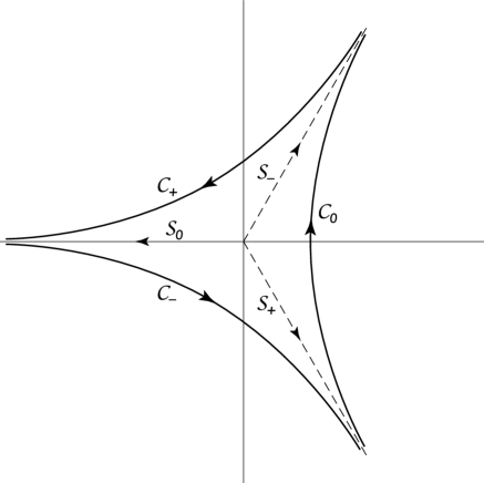
Figure 1: The complex-$t$ plane divided into three regions by the straight lines $\mathcal{S}_{-}$, $\mathcal{S}_{0}$ and $\mathcal{S}_{+}$, each subtending an angle of magnitude $2\pi/3$ with the others. The Airy integrals are defined along the infinite contours $\mathcal{C}_{-},~{}\mathcal{C}_{0}$ and $\mathcal{C}_{+}$, each of which asymptote to $\mathcal{S}_{-}$, $\mathcal{S}_{0}$ or $\mathcal{S}_{+}$ at infinity.

the integral being along an appropriate contour $\mathcal{C}$ in the complex-$t$ plane, which canonically is one of the curves $\mathcal{C}_{-},~{}\mathcal{C}_{0}$ or $\mathcal{C}_{+}$ depicted in Fig. 1. There are various ways of deriving this result, but they are not material to my presentation here. All that one need do is to substitute the representation (50) into equation (49) and show that it fits. There are three natural solutions, $y_{-}$, $y_{0}$ and $y_{+}$, represented by equation (50) on the contours $\mathcal{C}_{-}$, $\mathcal{C}_{0}$ and $\mathcal{C}_{+}$, respectively. Of course they cannot be independent, because equation (49) is of only second order. Since the integrand is entire, it follows that the integral along $\mathcal{C}_{-}\cup\mathcal{C}_{0}\cup\mathcal{C}_{+}$ vanishes, and therefore $y_{-}(x)+y_{0}(x)+y_{+}(x)=0$ for all (finite) $x$.

To span the solution space it is customary to adopt the two independent functions:

$${\rm Ai}(x)=y_{0}(x)~{},$$ (51)

evidently named after Airy (by Harold Jeffreys), and

$${\rm Bi}(x)=iy_{-}(x)-iy_{+}(x),$$ (52)

a not unnatural consequent appellation. Both functions are real for real $x$. It is Ai$(x)$ which is of principal interest here, for that is the solution that is relevant for our main purpose, for it decays, exponentially, for large positive (real) $x$. It can be obtained in terms of a single integral $I$ of a complex variable by deforming the contour $\mathcal{C}_{0}$ to $(-\mathcal{S}_{+})\cup\mathcal{S}_{-}$, on which $t=e^{-i\pi/3}s$ or $t=e^{+i\pi/3}s$ with $s$ real, whence

$$y_{0}(x)=\frac{1}{2\pi i}\left[e^{i\pi/3}I(e^{i\pi/3}x)-e^{-i\pi/3}I(e^{-i\pi/3}x)\right]~{},$$ (53)

which is evidently real when $x$ is real;

$$I(z):\,=\int^{\infty}_{0}e^{-zs-\frac{1}{3}s^{3}}{\rm d}s~{}.$$ (54)

The function Bi may be expressed similarly.

Series expansions of the Airy integral (50) were developed by Stokes (1864, 1871); Jeffreys and Jeffreys (1956) describe how to obtain asymptotic approximations for large $|x|$ by Debye’s method of steepest descents. When $x>0$, the saddle points in the complex-$t$ plane are at $t=\pm\sqrt{x}$, only the one on the positive real axis being accessible to ${\cal C}_{0}$. In its vicinity the line of steepest descents is parallel to the imaginary axis, and by deforming ${\cal C}_{0}$ to pass through $t=\sqrt{x}$ along that line one obtains immediately for ${\rm{Ai}}(x)$:

$${\rm Ai}(x)\sim\textstyle\frac{1}{2}\pi^{-1}x^{-\frac{1}{4}}\exp\left(-\frac{2}{3}x^{\frac{3}{2}}\right)\left[1+{\rm O}\left(x^{-1}\right)\right]$$ (55)

as $x\rightarrow+\infty$. If $x<0$, the saddles are at $t=\pm i\sqrt{-x}$, the lines of steepest descents being inclined at $\pm\pi/4$ from the real axis, respectively. Neither is accessible to ${\cal C}_{0}$, but we may evaluate $y_{\pm}$ instead and express $y_{0}$ as minus their sum: $y_{\pm}\sim\mp\left(2i\sqrt{\pi}\right)^{-1}(-x)^{-1/4}\exp\left[\pm i\left(\frac{2}{3}(-x)^{3/2}+\frac{\pi}{4}\right)\right]$,
whence

$${\rm Ai}(x)\!\sim\!\pi^{-\frac{1}{2}}(-x)^{-{\textstyle\frac{1}{4}}}\!\sin\!\left({\textstyle\frac{2}{3}}(-x)^{\frac{3}{2}}+{\textstyle\frac{1}{4}}\pi\!\right)[1+{\rm O}(x^{-1})]$$ (56)

as $x\rightarrow-\infty$.

The solution Bi$(x)$ grows exponentially as $x\rightarrow\infty$, as of course does any other combination of $y_{-}$, $y_{0}$ and $y_{+}$ that contains a nontrivial component of either $y_{-}$ or $y_{+}$. The particular combination (52) is chosen for defining Bi$(z)$ because it contains no exponentially small component in its asymptotic expansion as $x\rightarrow+\infty$.

The asymptotic analysis of ${\rm{Bi}}(x)$ for $x>0$ requires analysis in the vicinity of the saddle at $t=-\sqrt{x}$, through which the line of steepest descents is along the (negative) real axis. Both $\cal{C}_{+}$ and $\cal{C}_{-}$ can be distorted to pass through it, which leads to a doubling of the amplitude factor:

$${\rm Bi}(x)\sim\pi^{-\frac{1}{2}}x^{-\frac{1}{4}}\exp\left({\textstyle\frac{2}{3}}x^{\textstyle\frac{3}{2}}\right)[1+{\rm O}(x^{-1})]$$ (57)

as $x\rightarrow+\infty$. For $x<0$ one appropriately combines the expressions for $y_{-}$ and $y_{+}$ obtained previously to yield

$${\rm Bi}(x)\!\sim\!\pi^{-\frac{1}{2}}(-x)^{-\frac{1}{4}}\cos\left({\textstyle\frac{2}{3}}(-x)^{\frac{3}{2}}\!+\!{\textstyle\frac{1}{4}}\pi\right)\![1+{\rm O}(x^{-1})]$$ (58)

as $x\rightarrow-\infty$. Notice that the Wronskian of the asymptotic representations (55) and (57), and (56) and (58) takes the same constant value, $\pi^{-1}$, either side of the turning point, as it should.

One can develop expansions to higher order, but I do not do so here. I simply point out that for sufficiently large $x$ the relatively small correction to expression (57) at any order exceeds even the leading-order expression (55). Stokes’ realization was that it is because of that that one cannot analytically continue the leading-order expressions around the turning point and expect them still to represent the same solution of the differential equation (49).

Note that expression (56) provides the appropriate phase of the oscillatory branch of the solution in this relatively simple case, which was Stokes’s goal. But it does not yet answer the question for the more general equation (1). However, one should perhaps pause for a moment to appreciate the power of the argument in the Airy case. Although the asymptotic expressions (55)–(58) are necessarily only approximations, they are approximations to the exact representation (50), and the connexion between them is therefore robust. It isn’t even necessary to know what the functions look like for moderate or small values of $x$, where the conditions motivating the asymptotic expansions at large $|x|$ are not satisfied, although as a matter of natural curiosity one might wish to know. Accurate numerical solutions satisfy that desire. With such a connexion securely understood, Rayleigh (1912) applied the analysis of the Airy integral to a study of the reflection of waves propagating through a medium (actually a stretched membrane, for which equation (7) holds with $\omega_{\rm c}=0$) in which $c^{-2}$ varies linearly with $z$.

5.2 Jeffreys’ connexion

The connexion between the asymptotic representations of the solutions to the more general equation (1) either side of a turning point was first established by Jeffreys in his Cambridge Adams prize essay in 1923 (see also Jeffreys, 1925). Subsequently, interest in the issue arose in quantum mechanics with respect to solutions of the time-independent Schrödinger equation with a Coulomb potential, in studying, in particular, the asymptotic energy levels of the hydrogen atom.   Brillouin (1926) related Schrödinger’s equation to Hamilton-Jacobi theory of classical mechanics, and Wentzel (1926) discussed the leading-order LG expansion of Schrödinger’s equation; in response, Kramers (1926), who as an impoverished young man lived as a guest of the Jeffreys in their house in order to make ends meet during a stay in Cambridge, added the connexion formula that Harold Jeffreys had established. Mathematically their analysis was not new, but, being applied to a branch of physics that was more fashionable than the classical wave propagation that had interested Rayleigh and Jeffreys, it attracted the attention of more physicists (e.g. Young and Uhlenbeck, 1930; Kemble, 1935), and also mathematicians such as Langer (1934, 1937, 1949), and appellations combining the initials of the surnames of the three quantum physicists, in various orders, were given to the method, eventually converging on the order WKB. Yet later, when Jeffreys’ pioneering work was more widely recognized, the initial J was added, either in front or, more commonly, behind. I adopt the former, partly because Jeffreys has precedence, and partly because his analysis was designed to solve a wider class of problems than   merely  those  associated   with   the   time-independent
Schrödinger equation. It is interesting to contemplate, however, that had those who originally named this omnipresent and forgiving approximation been more aware of its true history, they might have dropped the initials W, K and B, and instead called it the SJ approximation.

There are now several ways of justifying the approximation (e.g. Heading, 1962). Jeffreys (1925) noted that if $f(z)$ has a simple zero at $z=z_{0}$, namely $f(z_{0})=0$ and $f^{\prime}(z_{0})\not=0$, then $f(z)\simeq f^{\prime}(z_{0})(z-z_{0})$ near $z=z_{0}$; and if $f^{\prime}(z_{0})>0$, the substitution $x=-k^{\frac{2}{3}}[f^{\prime}(z_{0})]^{\frac{1}{3}}(z-z_{0})$ transforms equation (1) approximately into Airy’s equation (49), which enables approximate solutions of the full equation to be likened to the exact solutions of the comparable approximate equation, and hence to a connexion between representations of the solutions either side of the turning point (via the integral representation (50)). He pointed out that the outcome is a limiting form of the true solution if $k$ is arbitrarily large. Thus the phase of that oscillatory solution in $z<z_{0}$ that connects to the solution that decays as $z\rightarrow+\infty$ is determined from equation (56).

Nowadays it is customary to use an approximation that is also valid far from the turning point. This is achieved by applying what has become known as the Liouville-Green transformation to equation (1), namely

$$x=-k^{\frac{2}{3}}{\rm sgn}(f)\left|{\textstyle\frac{3}{2}}\int^{z}_{z_{0}}f^{\frac{1}{2}}{\rm d}z\right|^{\frac{2}{3}}~{},$$ (59)

$$\Psi=\sigma\Phi:=(-xf^{-1})^{\frac{1}{4}}\Phi~{},$$ (60)

which leaves the equation in normal form. It may be written as

$$\frac{{\rm d}^{2}\Phi}{{\rm d}x^{2}}-x\Phi=k^{-2}h(x)\Phi~{},$$ (61)

where

$$h\{x[\sigma(z)]\}=-\sigma^{3}\frac{{\rm d}^{2}\sigma}{{\rm d}z^{2}}~{}.$$ (62)

First it should be noted again that near the turning point $f\simeq f^{\prime}_{0}(z-z_{0})~{},~{}{\rm where}~{}f^{\prime}_{0}=f^{\prime}(z_{0})$, and that therefore $x\sim-{\rm sgn}(f^{\prime}_{0})k^{\frac{2}{3}}|f^{\prime}_{0}|^{\frac{1}{3}}(z-z_{0})$, which is Jeffreys’ transformation: the term on the right-hand side of equation (61) arises from small higher-order terms in the Taylor expansion of $f$ about $z_{0}$, and can be neglected. Far from the turning point $f$ is no longer small, but, by definition, is of order unity. One can therefore estimate the ratio of the right-hand side of equation (61) to the second term on the left-hand side to be ${\rm O}(k^{-2}\sigma^{4}/xH^{2}_{f})\!=\!{\rm O}(k^{-2}H^{-2}_{f}f^{-1})={\rm O}(k^{-2}H^{-2}_{f})={\rm o}(1)$ as $k\rightarrow\infty$. Therefore, provided that $k$ is sufficiently large, the right-hand side can be ignored throughout, reducing equation (61) to Airy’s equation. What I have described here is not a proof, but it suggests that the solution, $\Phi={\rm Ai}(x)$, to what is now called the comparison (Airy) equation provides a valid approximation to the required solution of equation (1). And indeed Olver (e.g. 1974, 1978) has shown that for sufficiently well behaved functions $f$  the Airy-function approximation converges uniformly for all $x$ to the solution of equation (61) as $k\rightarrow\infty$.

It should be recalled that the JWKB procedure described above applies to simple turning points, for which $f^{\prime}(z_{0})\not=0$. If $f^{\prime}(z_{0})=0$ but $f^{\prime\prime}(z_{0})\not=0$, then one can carry out a similar analysis using Weber’s equation in the form ${\rm d}^{2}y/{\rm d}x^{2}$
$+x^{2}y=0$ as the comparison, and one may generalize further to yet higher-order turning points. Olver has proved uniform convergence in such cases too.

The uniformly valid JWKB approximation to the solution to equation (1) having a single simple turning point at $z=z_{0}$ such that $f>0$ for $z>z_{0}$ can therefore be written in terms of ${\rm Ai}(-x)$, where $x$ is defined by equation (59). Far from the turning point the appropriate asymptotic approximation (55) or (56) to the Airy function is applicable. It yields, after setting $f=\kappa^{2}$, as in §1, and relating $\Phi$ to $\Psi$ by equation (60),

$$\Psi\sim{\textstyle\frac{1}{2}}A|\kappa|^{-\frac{1}{2}}\exp(-\int^{z_{0}}_{z}|\kappa|{\rm d}z)~{}~{}{\rm for}~{}z\ll z_{0},$$ (63)

and

$$\Psi\sim A\kappa^{-\frac{1}{2}}\sin\left(\int^{z}_{z_{0}}\kappa{\rm d}z+\frac{\pi}{4}\right)~{}~{}{\rm for}~{}z\gg z_{0},$$ (64)

where $A$ is a constant amplitude. These are equivalent to the Liouville-Green expressions (19) and (16); but they are more precise, because they define which combination of the solutions (16) corresponds to the evanescent solution in $z<z_{0}$. It goes without saying that there is a similar pair of JWKB-approximate solutions that corresponds to exponential growth in the so-called evanescent zone. Such solutions would need to be combined with (63) and (64) if one were solving, for example, a barrier-penetration problem, either classical or quantum.

6 Equations with two well separated turning points: eigenvalue problems

Few sharp boundaries are encountered in astrophysics. Normally, in wave problems, when waves are confined within some region $\mathcal{P}$ it is because they encounter other, bounding, regions $\mathcal{E}$ into which they cannot propagate, but the ‘interface’ is of finite thickness and is smooth. (I have in mind a 3-dimensional space with propagating and evanescent regions $\mathcal{P}$ and $\mathcal{E}$ separated by 2-dimensional surfaces.) That is not to say that no wave at all can propagate in the bounding regions $\mathcal{E}$. Usually the bounding regions can support waves of the same type as those under consideration, but with rather different frequency or wave number. The ‘boundary’ $\mathcal{B}$ between those regions can usually be regarded as the location of a turning point (or, more generally, as the locus of a turning point), in the sense that I have used it in this article, and is as well defined as are the critical cutoff frequencies.

I confine my discussion to situations in which the background state is independent of time, so that frequency $\omega$ is well defined, and is conserved, as is wave energy in a dissipationless system. (An LG expansion in time, and even a JWKB approximation, can be made to study waves in an appropriately slowly changing environment, but I do not address that here.) Consider there to be a set of locally Cartesian coordinates $(\xi,\eta,\zeta)$ established in the vicinity of the boundary, with $\zeta$ perpendicular to the boundary. (The co-ordinate $\xi$ here is not to be confused with the vertical component of the displacement of equation (33).) Generically, the background (equilibrium) state varies more rapidly with $\zeta$ than it does with $\xi$ and $\eta$ (there are exceptions). On a length scale smaller than the scale of variation on $\mathcal{B}$ of the background state, the differential equation describing the waves reduces approximately to an ordinary (linear) differential equation with respect to $\zeta$ (often of second order, analogous to equation (1), the only case I consider explicitly here), with a turning point ‘on’ $\mathcal{B}$. Why does that turning point arise? In other words, why is wave propagation possible in $\mathcal{P}$ but not in $\mathcal{E}$?

One reason might be that no wave of frequency $\omega$ can propagate in $\mathcal{E}$, whatever its orientation. Then a wave incident on $\mathcal{B}$ has its direction reversed – equation (1) permits no other possibility – undergoing what is called (true) reflection. Alternatively, $\mathcal{E}$ simply doesn’t permit continued propagation of a wave with a particular angle of incidence: if the background state is independent of some particular coordinate $\xi$ (or $\eta$, it cannot be $\zeta$), then the component $k_{\xi}$ of the local wavenumber is conserved across the boundary, and if $f$ in equation (1) is then rendered negative in $\mathcal{E}$ for that value of $k_{\xi}$ (at the frequency $\omega$ of the wave), propagation is impossible; indeed, because the variation of the background state is gentler in $\mathcal{B}$ than perpendicular to it, that describes approximately the situation with respect to the entire component $k_{\perp}$ of the wavenumber in $\mathcal{B}$ (i.e. perpendicular to the normal). The process is often called total internal reflection, and, if $f$ is continuous, the case first considered by Rayleigh (1912), can be thought of as the result of continuous refraction in the vicinity of $\mathcal{B}$. Note that because the exponents of the two LG solutions (16) have the same magnitude at any point, the angle of reflection is equal to the angle of incidence. Note also that, because $f$ varies when either $\omega$ or $k_{\perp}$ vary (at given $\zeta$), the location of $\mathcal{B}$ varies with not only frequency but also with the angle of incidence of the wave; and, for some values of $\omega$ and $k_{\perp}$, $\cal B$ may not exist.

A region $\mathcal{P}$ that is enclosed by $\mathcal{E}$ is called a cavity. Any wave confined within it, in the absence of dissipation, will, under most situations, eventually pass arbitrarily close to any point it had passed formerly, and interfere with itself. For certain frequencies, that interference is constructive everywhere in $\mathcal{P}$, and resonance occurs. The resulting motion is called a mode of oscillation: the contents of the entire region $\mathcal{P}$ oscillate in unison with frequency $\omega$ (it being quiescent elsewhere). For sufficiently high $k$ the LG expansion can be used along the phase trajectories of the waves, using JWKB theory in the vicinity of the boundary of $\mathcal{P}$, to determine the values of $\omega$ that permit resonance. These values are called the eigenfrequencies of the cavity. Such an analysis can be geometrically complicated enough to detract from the main point of this discussion, so I postpone discussion of the general problem to another article. Here I simply consider a problem in just one dimension, in which a wave after reflection is bound to pass through all the points it had passed through previously. Then the governing differential equation is of the type (1), with $k$ and $f$ depending in some way on $\omega$.

To be more specific,  let us consider a situation in which $f(z)=\kappa^{2}>0$ for $z_{1}<z<z_{2}$, and $f<0$ elsewhere. Asymptotic solutions $\Psi_{2}(z)$ in the vicinity of $z_{2}$, and far from $z_{1}$, may be written as $\sigma(x)\Phi_{2}(x)$, where $x$ is defined by equation (59) with $z_{0}$ replaced by $z_{2}$, $\sigma$ is defined by equation (60), and $\Phi(x)={\rm Ai}(x)$. In the vicinity of $z_{1}$ one may do likewise to define $\Psi_{1}(z)=\sigma(x)\Phi_{1}(x)$, but with $x$ defined with the opposite sign, and now with $z_{0}$ replaced by $z_{1}$, to ensure that the interval in which Ai is oscillatory satisfies $z>z_{1}$. For simplicity I shall assume that $z_{1}$ and $z_{2}$ are sufficiently far apart that there is a common region of validity in $(z_{1},z_{2})$ of the high-$(-x)$ expansion (55) of $\Phi_{1}$ and $\Phi_{2}$. This must be possible for sufficiently large $k$. Then $\Psi_{1}$ and $\Psi_{2}$ can be matched. According to equation (64),

$$\Psi_{1}\sim A_{1}\kappa^{-\frac{1}{2}}\sin\left(k\int^{z}_{z_{1}}\kappa{\rm d}z+{\textstyle\frac{\pi}{4}}\right)~{}{\rm for}~{}z \gg z_{1}$$

$$({\rm and}~{}z \ll z_{2})$$ (65)

and

$$\Psi_{2}\sim A_{2}\kappa^{-\frac{1}{2}}\sin\left(k\int^{z_{2}}_{z}\kappa{\rm d}z+{\textstyle\frac{\pi}{4}}\right)~{}{\rm for}~{}z \ll z_{2}$$

$${\rm(and}~{}z \gg z_{1})~{}.$$ (66)

The  representations are identical throughout the common interval of validity if $A_{2}=\pm A_{1}$ and

$${\sin\atop\cos}\left({\textstyle\frac{1}{2}}k\int^{z_{2}}_{z_{1}}\kappa{\rm d}z+{\textstyle\frac{\pi}{4}}\right)=0~{},$$ (67)

which is possible only if

$$k\int^{z_{2}}_{z_{1}}\kappa{\rm d}z=\left(n-{\textstyle\frac{1}{2}}\right)\pi~{},$$ (68)

where $n$ is an integer, and, in order to achieve a possible matching with the two evanescent solutions either side of the oscillatory region, at least one half-wavelength is required:  therefore $n=1,2,3,\ldots~{}$. This is the desired eigenvalue equation.

I promised to illustrate the approximation with acoustic-gravity modes of a star, for which, in the case of a spherical star, $k\kappa$ is $K$ given by equation (37). I do so with some hesitation, however, because stars are not quite as simple as the situation I have just discussed. The reason is that if $\omega$ is high, which is one way of making $K$ large, then the upper turning point $r_{2}$, which occurs roughly where $\omega^{2}_{\rm c}(r)=\omega^{2}$, is close to the surface, towards which $\omega^{2}_{\rm c}$, and perhaps also $N^{2}$ (depending on whether or not the outer layers are convective, although the $\omega^{2}$ dividing $N^{2}$ makes its effect relatively small), rise rapidly, as though they are approaching a singularity located at what I call the seismic surface of the star. This is a structural property of all stars. In practice, where the outer layers become optically thin, the stratification becomes approximately isothermal, and therefore essentially exponential, and the singularity that would be encountered in a polytrope, for example, is avoided. Nevertheless, for many modes, with $\omega$ rather less than the value of $\omega_{\rm c}$ in the photosphere, the transition to exponential behaviour occurs sufficiently well beyond the upper turning point for its presence to be hardly discernible in the dynamically active propagating regions below. Therefore the solution to equation (1) actually feels the influence of the phantom singularity, and the eigenvalue equation (68) needs adjustment. How that is achieved is beyond the scope of this elementary introduction, and is postponed to a subsequent article. Here I simply assume that $\omega$ is not so high as to make that adjustment necessary. There is also a similar problem near the centre, where $L^{2}/r^{2}$ suffers a true (co-ordinate) singularity. This is a geometrical property of any wave problem in a sphere, and was first encountered in the context of JWKB theory in quantum mechanics (with a Coulomb potential). That singularity is well avoided if the degree $l$ of the spherical harmonic (the angular-momentum quantum number in quantum mechanics) is sufficiently large, so that the lower turning point $r_{1}$, which is determined approximately for high-frequency (acoustic) modes by $r_{1}/c(r_{1})=L/\omega$, is not very close to the centre. Similar problems face gravity modes, which have very low frequency, although the problem near the surface of the star is present only in stars with radiative envelopes, for otherwise the modes are shielded from the surface by the evanescent convection zone in which $N^{2}\leq 0$.

With these caveats in mind, I now intrepidly make the substitution $k\kappa=K$ in equation (68), using equation (37) to obtain

$$\int^{\tau_{2}}_{r_{1}}\left[\frac{\omega^{2}-\omega^{2}_{\rm c}}{c^{2}}-\frac{L^{2}}{r^{2}}\!\left(\!1-\frac{N^{2}}{\omega^{2}}\right)\!\right]^{\frac{1}{2}}\!{\rm d}r\!\sim\!\left(n-{\textstyle\frac{1}{2}}\right)\pi~{},$$ (69)

hoping that a range of $\omega$ exists which is high enough for the LG expansion to be reasonably accurate and low enough for the JWKB approximation near the turning points not to be unduly disturbed by singularities, phantom or real.

For acoustic modes $\omega^{2}$ is large, and for many purposes $N^{2}/\omega^{2}$ may be neglected compared with unity, yielding

$$\frac{\left(n-\frac{1}{2}\right)\pi}{\omega}\sim\int^{\tau_{2}}_{\tau_{1}}\left(1-\frac{\omega^{2}_{\rm c}}{\omega^{2}}-\frac{c^{2}}{r^{2}w^{2}}\right)^{\frac{1}{2}}{\rm d}\tau~{},$$ (70)

where $\tau_{1}=\tau(r_{1}),~{}\tau_{2}=\tau(r_{2})$ and $w=\omega/L$; for gravity modes $\omega^{2}/c^{2}$ may often be neglected, yielding

$$\frac{\left(n-\frac{1}{2}\right)\pi}{L}\sim\int^{r_{2}}_{r_{1}}\left(\frac{N^{2}}{\omega^{2}}-1-\frac{r^{2}\omega^{2}_{\rm c}}{L^{2}c^{2}}\right)^{\frac{1}{2}}\frac{{\rm d}r}{r}~{},$$ (71)

in both cases the turning points $r_{1}$ and $r_{2}$ being interpreted as the points at which the integrands vanish.

It is interesting to develop equation (70) further in the case when $L$ is large, for then the lower turning point is close enough to the surface for the effect of the spherical geometry to be small. In that case one may regard the horizontal phase velocity $v_{\phi\rm h}=rw$ to be essentially independent of $r$. If, in addition, one approximates the surface layers of a star of seismic radius $R$ by a plane-parallel polytrope of index $\mu$, so that $c^{2}=\gamma_{1}gz/(\mu+1)$ and $\omega^{2}_{\rm c}=\mu(\mu+2)\gamma_{1}g/4(\mu+1)z$, where $z=R-r$ is depth beneath the seismic surface of the star (e.g. Gough, 1993), then the acoustic depth $\tilde{\tau}$ beneath the seismic surface is given by $\tilde{\tau}=2z/c$, and $\omega^{2}_{\rm c}=\mu(\mu+2)/\tilde{\tau}^{2}$. Equation (70) reduces to

$$\frac{\left(n-\frac{1}{2}\right)\pi}{\omega} \sim \int^{\tilde{\tau}_{2}}_{\tilde{\tau}_{1}}\left[1-\frac{\mu(\mu+2)}{\omega^{2}\tilde{\tau}^{2}}-\frac{\gamma_{1}^{2}g^{2}\tilde{\tau}^{2}}{4(\mu+1)^{2}v_{\phi\rm h}^{2}}\right]^{\frac{1}{2}}{\rm d}\tilde{\tau}$$ (72)

$$= \left[\frac{(\mu+1)v_{\phi\rm h}}{2\gamma_{1}g}-\frac{{\sqrt{\mu(\mu+2)}}-2}{2\omega}\right]\pi~{},$$

in which $\tilde{\tau}_{1}$ and $\tilde{\tau}_{2}$ are respectively the acoustic depths of the upper and lower turning points. This equation may be rewritten

$$\frac{(n+\alpha)\pi}{\omega}=F(v_{\phi\rm h})~{},$$ (73)

where $F(v):=(\mu+1)\pi v/2\gamma_{1}g$ and $\alpha=\frac{1}{2}[\sqrt{\mu(\mu+2)}-1]=$ constant, which is a special case of what is now known as Duvall’s law (1982), namely equation (73) with the functional form of $F$ unspecified and with the constant $\alpha$ not necessarily related directly to a polytropic index, and which formally describes high-frequency acoustic modes in a stellar envelope with a (well behaved) reflecting surface, whatever its stratification. The polytropic form derived here can be rewritten $\omega^{2}\sim(n+\alpha)\tilde{\omega}^{2}_{0}Rk$ as $k\rightarrow\infty$, where $\tilde{\omega}^{2}_{0}=2\gamma_{1}g/(\mu+1)R$ is the square of a characteristic acoustic frequency of the outer layers of the star, and here $k=L/R$ is the horizontal wavenumber at the surface. This is the parabolic form which approximates the solar $k-\omega$ relation familiar to helioseismologists, and was used to provide the first seismic calibration of the adiabatic constant deep in the solar convection zone. The more general form of equation (73) when the polytropic sound-speed variation is not assumed can be inverted to give $c/r$ as a function of the observables $(n+\alpha)\pi/\omega$ and $w$ (e.g. Gough, 1993), and was used to provide the first inferences of the sound speed through the Sun.

7 Closing words

The JWKB approximation provides a wonderfully robust representation of the waves encountered throughout physics. Turning points are very common, and, provided one is well clear of them, the approximation reduces to simple formulae in terms of an exponential function on one side, and a trigonometrical function on the other, together with the connexion formula providing the value of the phase of the trigonometrical function according to whether the exponential function grows or decays away from the turning point. Even near the turning point, it is straightforward to evaluate the Airy-function representation from which these simpler formulae are derived.

In solar physics, the leading term in the LG expansion, now commonly called the WKB approximation, is almost ubiquitous in studies of waves in the atmosphere, and when turning points are encountered the more powerful JWKB approximation is available.  For  internal  acoustic-gravity waves at least one turning point, $r_{1}$, is always present, and the connexion formula provided by the JWKB approximation is essential. I have discussed the latter explicitly, showing how, if $\omega$ is low enough for the waves to be trapped inside the Sun by reflection near the surface, the approximate equation (69) determines the eigenfrequencies of the resonant modes. In the case of acoustic modes of the Sun and Sun-like stars, that formula is only approximate. There are two reasons: (i) if $\omega$ is low enough for the upper turning point not to be too close to the phantom singularity at the seismic surface of the Sun, then one runs the risk of not having $k$ large enough for the Airy equation (61) with the right-hand side ignored to provide a reliable comparison to the full equation. That risk is usually small, because in most (but not all) cases the Airy-function representation is amazingly robust; (ii) if the frequency is high, not only does the upper turning point approach the acoustic surface of the Sun, but it also encounters the upper superadiabatic boundary layer of the convection zone where, over a small distance, the acoustic cutoff frequency becomes imaginary; then there appear to be three turning points which are too close together for the technique described in §6 for piecing together different Airy functions to be applicable. In that case special attention beyond the scope of this introduction is required, but I might at least point out that it is pertinent to the interpretation of observational investigations of the transition to supercriticality, namely to the high-frequency domain exceeding the acoustic cutoff frequency in the atmosphere. In the case of gravity waves in a star with a convective envelope, the threat of a singularity occurs only near the lower turning point, although in the absence of a convective envelope, the surface threatens too.

It is worth mentioning that the leading-order LG expansion is formally applicable only in the limit of infinitesimally slow variation of the function $f$ in equation (1). It therefore does not capture reflection. The JWKB approximation behaves likewise, except near the turning point. Reflection in a spatially varying propagating region is likely to occur everywhere to some degree, but it is significant only when the scale of variation $H_{f}$ of the background state is comparable with or much smaller than the characteristic inverse wavenumber $(kf^{\frac{1}{2}})^{-1}$ of the wave. When it is much smaller the variation may be regarded as a discontinuity, across which one can match two JWKB solutions, in the manner adopted by Poisson (1817) under conditions when the simpler approximation obtained by taking $f$ to be piecewise constant is  applicable.    If $kf^{\frac{1}{2}}H_{f}\approx 1$ over an extended region, one might need to adopt a more complicated comparison equation for the JWKB approximation: to deal with a simple smooth barrier between $z_{1}$ and $z_{2}$, for example, one can adopt Weber’s equation in the form $y^{\prime\prime}+k^{2}(z-z_{1})(z-z_{2})y=0$ (e.g. Langer, 1959); more complicated variations in $f$ require correspondingly more complicated comparison equations. One  must consider in such cases whether the result would justify the effort, because direct numerical solution of an ordinary differential equation is much more straightforward, even when there are singularities present.

Whether the result justifies the effort depends on the use to which one wishes to put the result. If all one needs are eigenfunctions and their corresponding eigenvalues, the direct numerical computation is in many cases simpler and more reliable. But analytical results are, for many a person, easier to interpret. And then it is more likely that one could be able to put them to good use. For example, in the early days of helioseismology, the significance of the so-called large and small frequency separations of low-degree acoustic modes was first recognized from an asymptotic analysis, as subsequently, in a sense, was the Duvall law (1982), use of which has been central to many helioseismological investigations. It has been argued by some helioseismologists that asymptotic analysis was actually unnecessary because the discoveries could equally have been made by numerical investigation. Perhaps they could. But the fact of the matter is that they were not, and that progress in the subject would undoubtedly have been slower without asymptotics. That mode of discovery is likely to continue: the days of asymptotic analysis in stellar physics are certainly not gone.

References

- [1] Booker, J.R., Bretherton, F.P.: 1967, J. Fluid Mech. 27, 513–539
- [2] Brillouin, L.: 1926, Comptes Rend. Acad. Sci. Paris 183, 24–26
- [3] Carlini, F.: 1817, Giorn. Fis. Chim. Storia Nat. Med. Arti 10, 458-460
- [4] Christensen-Dalsgaard, J., Cooper, A.J., Gough, D.O.: 1983, Mon. Not. Roy. Astron. Soc. 203, 165–179
- [5] Deubner, F-L., Gough, D.O.: 1984, Ann. Rev. Astron. Astrophys. 22, 593–619
- [6] Duvall Jr, T.L.: 1982, Nature 300, 242–243
- [7] Fröman, N., Fröman, P.O.: 1996, Phase-Integral Methods Allowing Near-lying Transition Points, Springer Tracts in Nat. Phil. 40, Springer, Heidelberg
- [8] Gough, D.O.: 1993, in Astrophysical Fluid Dynamics (ed. J-P. Zahn & J. Zinn-Justin), Elsevier, Amsterdam 399–560
- [9] Green, G.: 1837, Trans. Camb. Phil. Soc. 6, 457–462
- [10] Heading, J.: 1962, An Introduction to phase-integral methods, Methuen, London
- [11] Jeffreys, H.: 1925, Proc. Lond. Math. Soc. 2nd Ser. 23, 428–436
- [12] Jeffreys, H., Swirles, B. (Lady Jeffreys): 1956, Methods of Mathematical Physics, Cambridge University Press, Cambridge
- [13] Kemble, E.C.: 1935, Phys. Rev. 48, 549–561
- [14] Kramers, H.A.: 1926, Zs Phys. 39, 828–840
- [15] Lamb, H.: 1909, Proc. Lond. Math. Soc. 2nd Ser. 7, 122–141
- [16] Langer, R.E.: 1934, Bull. Am. Math. Soc. 40, 545–582
- [17] Langer, R.E.: 1937, Phys. Rev. 51, 669–676
- [18] Langer, R.E.: 1949, Trans. Amer. Math. Soc. 67, 461–490
- [19] Langer, R.E.: 1959, Trans. Amer. Math. Soc. 90, 113–142
- [20] Larmor, J. (arr.): 1907, Memoir and Correspondence by the late Sir George Gabriel Stokes, Bart, Cambridge University Press, Cambridge, p.62
- [21] Liouville, J.: 1837, J. Math. pures appl. 2, 16–35
- [22] Olver, F.W.J.: 1974, Asymptotics and Special Functions, Academic Press, New York
- [23] Olver, F.W.J.: 1978, Phil. Trans. Roy. Soc. London 289, 501–548
- [24] Poisson, M.: 1817, Mém. Acad. Roy. Soc. Inst. France 2, 305–402
- [25] Rayleigh: 1912, Proc. Roy. Soc. London A86, 207–226
- [26] Reye, T.: 1872, Die Wirbelstürme, Tornados und Wettersaulen, Genesius, Halle
- [27] Schmitz, F., Fleck, B.: 1998, Astron. Astrophys. 337, 487–494
- [28] Stokes, G.G.: 1864, Trans. Camb. Phil. Soc. 10, 105–128
- [29] Stokes, G.G.: 1871, Trans. Camb. Phil. Soc. 11, 412–425
- [30] Wentzel, G.: 1926, Zs Phys. 38, 518–29
- [31] Young, L.A., Uhlenbeck, G.E.: 1930, Phys. Rev. 36, 1154–1167