The Most Massive Black Holes in the Universe:
Effects of Mergers in Massive Galaxy Clusters

Abstract

Recent observations support the idea that nuclear black holes grew by gas accretion while shining as luminous quasars at high redshift, and they establish a relation of the black hole mass with the host galaxy’s spheroidal stellar system. We develop an analytic model to calculate the expected impact of mergers on the masses of black holes in massive clusters of galaxies. We use the extended Press-Schechter formalism to generate Monte Carlo merger histories of halos with a mass $10^{15}{h^{-1}M_{\odot}}$. We assume that the black hole mass function at $z=2$ is similar to that inferred from observations at $z=0$ (since quasar activity declines markedly at $z<2$), and we assign black holes to the progenitor halos assuming a monotonic relation between halo mass and black hole mass. We follow the dynamical evolution of subhalos within larger halos, allowing for tidal stripping, the loss of orbital energy by dynamical friction, and random orbital perturbations in gravitational encounters with subhalos, and we assume that most black holes will efficiently merge after their host galaxies (represented as the nuclei of subhalos in our model) merge. Our analytic model reproduces numerical estimates of the subhalo mass function. We find that mergers can increase the mass of the most massive black holes in massive clusters typically by a factor $\sim$ 2, after gas accretion has stopped. In our ten realizations of $10^{15}{h^{-1}M_{\odot}}$ clusters, the highest initial ($z=2$) black hole masses are $5-7\times 10^{9}M_{\odot}$, but four of the clusters contain black holes in the range $1-1.5\times 10^{10}M_{\odot}$ at $z=0$. Satellite galaxies may host black holes whose mass is comparable to, or even greater than, that of the central galaxy. Thus, black hole mergers can significantly extend the very high end of the black hole mass function.

1. Introduction

The idea that quasars are powered by accretion of gas in a disk orbiting a massive black hole (Salpeter, 1964; Zel’dovich & Novikov, 1964; Lynden-Bell, 1969) requires that enough black holes should exist at the present time to account for all the mass that had to be accreted over the past history of the universe by all observed quasars (Sołtan, 1982). Much progress has been made over the last decade by discovering black holes in galactic nuclei, measuring their masses and characterizing the population (Magorrian et al. 1998). Using the surprisingly tight relation that is observed between the black hole mass and the velocity dispersion of the spheroidal stellar population of the host galaxy (Ferrarese & Merritt 2000; Gebhardt et al. 2000; Tremaine et al. 2002 and references therein), one finds that the average mass density of the population of nuclear black holes is roughly equal to what is required for the amount of light that has been emitted by all Active Galactic Nuclei (AGN), if the radiative efficiency is close to 10%, a typical value expected for geometrically thin accretion disks (see, e.g., Barger et al. 2001; Yu & Tremaine 2002; Shankar et al. 2006). This implies (with the caveat of the substantial observational uncertainties that are still present in the determination of the black hole mass density and the integrated AGN emission) that a major contribution to the growth of the black hole mass density is the accretion of gas that is responsible for AGN, and that contributions from radiatively inefficient accretion (which may arise in super-Eddington or strongly sub-Eddington accretion flows) are at most comparable to the accretion from geometrically thin disks.

Black hole mergers do not change the total mass density in the black hole population, so they do not alter this argument, but they can alter the mass distribution of black holes. Observationally, we have relatively little handle on the black hole mass function outside the range $10^{7}-10^{9}M_{\odot}$ that dominates the average mass density. The most luminous quasars of which we have evidence at high redshift imply black hole masses close to $10^{10}M_{\odot}$ (e.g., Fan et al. 2003), assuming they are radiating at the Eddington luminosity. The most massive black hole discovered so far is in M87, with a mass of $M_{\bullet}\sim 3\times 10^{9}M_{\odot}$. It is natural to assume that the highest mass black holes may be lurking in some of the most massive elliptical galaxies, but we do not know whether the power-law $M_{\bullet}-\sigma$ correlation extends up to these largest black hole masses. Similar uncertainties plague the determination of the abundance of low-mass black holes.

A number of interesting questions can be raised in relation to theoretical expectations for the most massive black holes. Under the assumption that the Eddington luminosity cannot be exceeded (a point recently questioned by Begelman, Volonteri & Rees [2006]), what is the abundance of the most massive black holes we should expect? Do the cold dark matter models for structure formation predict that the most massive black holes should generally reside in central cluster galaxies, or can they sometimes reside in a massive galaxy that has only recently merged in a cluster, still moving in the cluster outskirts? How much could the most massive black holes have grown by mergers? If we search today for black holes in the central cluster galaxies of the most massive clusters, what is the black hole mass we should expect to measure?

With these questions in mind, in this paper we develop a dynamical model for the evolution of the supermassive black hole population. We use this model to examine the effect of black hole mergers on the high-mass end of the present-day mass distribution. The model we develop aims to treat carefully the dynamics of a halo containing a central black hole once it becomes an orbiting satellite within a larger halo. The problem of the merger of two central black holes after their halos are merged will not be considered here, and we simply obtain the maximum merger rate by assuming that two black holes will always merge on a short time scale once they become bound to each other in the center of two merging halos. After the host halo of a black hole’s parent galaxy merges into a bigger halo, it becomes an orbiting subhalo. The subhalo may either remain in orbit indefinitely (in which case the black hole will not merge), or it may be dragged by dynamical friction to the center of the larger halo within which it is orbiting and be tidally disrupted. In the latter case, a black hole merger may ensue. We will present the result of a model where black holes are initially distributed among host halos after they have been formed by gas accretion, and then their mergers are followed according to the dynamical evolution of their subhalos. Our model is similar to that of Volonteri, Haardt & Madau (2003), though we treat the dynamical evolution of the subhalos in greater detail. We shall focus in this paper on the black holes that are present in a halo of $10^{15}{h^{-1}M_{\odot}}$ at the present time, representing a massive galaxy cluster.

Our implementation of a merger tree for dark matter halos is described in § 2, and the method to follow the dynamical evolution of merged subhalos is explained in § 3 and § 4. In § 5, we specify the initial conditions by which we populate halos with black holes of different masses at an initial redshift. The results on the importance of mergers for black holes in clusters, and the masses of the central black holes, are presented in § 6 and discussed in § 7.

2. Properties of Dark Matter Halos

We develop in this paper a dynamical model of substructure in dark matter halos. The first step is to construct a merger tree, starting from a present day halo (which for the application explored in this paper will represent a halo like that of the Coma cluster) and going backwards in time to generate all the merger events. This section describes how the merger tree is generated, how each halo in the tree is assigned a mass and a radius, and the choice we make for the halo density profiles. In § 3, we describe the second step, where we follow the dynamical evolution of the halos after they have become satellites of a larger halo, starting at the earliest time when the first low-mass halos form, and moving forward to the present time.

2.1. Merger History

We use the extended Press-Schechter formalism to generate the merger tree (Press & Schechter, 1974; Bond et al., 1991). This formalism is very simple to use and is known to provide an adequate description for a merger history of a halo of mass comparable to the Milky Way galaxy (e.g., Bullock, Kravtsov & Weinberg 2000), although in detail there are deviations of the halo mass function from the results of numerical simulations (e.g., Eke, Cole & Frenk 1996; Sheth & Tormen 1999; Jenkins et al. 2001).

We define $n(M,z)$ as the number density of halos of mass greater than $M$ at redshift $z$, and $\sigma(M,z)$ as the extrapolated linear rms fluctuation in spheres containing an average mass $M$. The halo number density is related to the fraction of the mass that is in halos of mass $M$ per unit $\ln\sigma(M)$ by

$$f(\sigma,z)={M\over\bar{\rho}_{m}}{dn(M,z)\over d\ln\sigma},\vspace{10pt}$$ (1)

where $\bar{\rho}_{m}$ is the mean matter density of the universe. The Press-Schechter model assumes that

$$f=\sqrt{2\over\pi}{\delta_{c}\over\sigma}\exp\left(-{\delta_{c}^{2}\over 2\sigma^{2}}\right),\vspace{10pt}$$ (2)

where $\delta_{c}(z)$ is the critical threshold on the linear overdensity for collapse at $z$. We adopt the approximate fitting formula for $\delta_{c}(z)$ of Eke, Cole, & Frenk (1996; see also, Carroll, Press & Turner 1992) for a $\Lambda$CDM universe. The idea for the merger tree is based on the conditional probability that a particle in a halo of mass $M_{2}$ at redshift $z_{2}$ was part of a halo of mass $M_{1}$ at redshift $z_{1}(>z_{2})$ (Lacey & Cole, 1993; Cole et al., 2000).

$$f_{12}(M_{1},M_{2})dM_{1} = {1\over\sqrt{2\pi}}{{(\delta_{c1}-\delta_{c2})}\over{(\sigma^{2}_{1}-\sigma^{2}_{2})^{3/2}}}$$ (3)

$$\times\exp\left[-{{(\delta_{c1}-\delta_{c2})^{2}}\over{2(\sigma^{2}_{1}-\sigma^{2}_{2})}}\right]{{d\sigma^{2}_{1}}\over{dM_{1}}}dM_{1},$$

where each subscript indicates the corresponding redshift. Then, the mean number of halos of mass $M_{1}$ that merge into a halo of mass $M_{2}$ over a time step $dt_{1}$ is $dN/dM_{1}=(df_{12}/dt_{1})(M_{2}/M_{1})\,dt_{1}$. The merger tree with mass resolution $M_{\rm res}$ is built by generating new progenitors of mass $M_{\rm res}<M_{1}<M_{2}/2$ with total probability $P$ given by (Cole et al., 2000)

$$P=\int_{M_{\rm res}}^{M_{2}/2}{{dN}\over{dM_{1}}}\,dM_{1}~{},\vspace{10pt}$$ (4)

and adding a rate of smooth mass accretion, $F$, equal to

$$F=\int_{0}^{M_{\rm res}}{{dN}\over{dM_{1}}}{M_{1}\over M_{2}}\,dM_{1}~{},\vspace{10pt}$$ (5)

to account for the mass of unresolved halos with $M_{1}<M_{\rm res}$ that are not discretely generated.

2.2. Density Profile

Density profiles of halos from numerical simulations have been fitted to a variety of forms (Navarro, Frenk & White, 1997; Moore et al., 1999; Fukushige & Makino, 2001; Navarro et al., 2004). Here we will be interested in describing profiles of satellite halos with finite mass after they have merged into a larger halo. The profile of Navarro, Frenk & White (1997) has a density slope $d\log\rho/d\log r$ approaching 3 at large radius, giving rise to a logarithmic divergence of the total mass, which demands the introduction of a cutoff radius. We adopt instead the simple form of the Jaffe sphere:

$$\rho_{\rm h}(r)=\left({M_{\rm h}\over{4\pi R_{\rm h}^{3}}}\right){R_{\rm h}^{4}\over{r^{2}(r+R_{\rm h})^{2}}}~{},\vspace{10pt}$$ (6)

where the Jaffe radius $R_{\rm h}$ is defined as the radius inside which the mass is half of the total halo mass $M_{\rm h}$. This profile is steeper than that found in purely collisionless numerical simulations in the central part, but it has the advantage of describing a finite mass halo with a very simple form for the potential. In addition, black holes should in reality be in the center of a galaxy, and the baryonic component will steepen the profile near the center making it closer to that of a Jaffe sphere.

In later sections, we will be using the one-dimensional velocity dispersion of the Jaffe sphere at each radius for isotropic orbits, which is found from the spherical Jeans equation (Binney & Tremaine, 1987) to be

$$\sigma^{2}(r) = -{6GM_{\rm h}\over R_{\rm h}}\left({r\over R_{\rm h}}\right)^{2}\left(1+{r\over R_{\rm h}}\right)^{2}\ln\left({r\over{r+R_{\rm h}}}\right)$$

$$-{GM_{\rm h}\over 2R_{\rm h}}\left[12\left({r\over R_{\rm h}}\right)^{3}+18\left({r\over R_{\rm h}}\right)^{2}+4\left({r\over R_{\rm h}}\right)-1\right].$$

2.3. Radii of Dark Matter Halos

The evolution of a halo of mass $M_{\rm h}$ after it merges with another object depends not only on its mass, but on its half-mass radius $R_{\rm h}$ as well, because in general denser objects will be less vulnerable to tidal disruption and will more easily survive as orbiting satellites. It is therefore important to estimate the radius of a halo as it evolves, first by acquiring new mass through mergers and accretion, and then by losing mass through tidal disruption once it has been incorporated into a larger halo as a satellite.

When a halo first appears in the merger tree at the resolution mass $M_{\rm res}$, we assign an initial radius to the halo, assuming the standard collapse model in which a spherical top-hat overdense region turns around from the Hubble expansion at radius $R_{\rm t}$, and then virializes at a collapse radius $R_{\rm col}=R_{\rm t}/2$. We use the fitting formula of Bryan & Norman (1998) for the mean density of the non-linear collapsed object, $\rho_{\rm col}=\rho_{\rm crit}(z)\Delta_{\rm col}$, where $\rho_{\rm crit}$ is the critical density at the redshift $z$ of collapse, the mean matter density is $\rho_{m}(z)=\Omega_{m}(z)\rho_{\rm crit}$, and a flat cosmological model is assumed:

$$\Delta_{\rm col}=18\pi^{2}+82x-39x^{2},~{}~{}~{}x=\Omega_{m}(z)-1~{}.\vspace{10pt}$$ (8)

The collapse radius is obtained from

$$M_{\rm h}={4\pi\over 3}\,R_{\rm col}^{3}\rho_{\rm col}~{}.\vspace{10pt}$$ (9)

For the Jaffe density profile of halos we will be assuming in this paper, the Jaffe radius $R_{\rm h}$ that corresponds to this collapse radius is obtained by equating the initial potential energy of a homogeneous sphere at the turnaround radius $R_{\rm t}=2R_{\rm col}$ to half of the potential energy of the Jaffe sphere, which gives

$$R_{\rm h}={5\over 6}\,R_{\rm col}={5\over 12}\,R_{\rm t}~{}.\vspace{10pt}$$ (10)

However, as halos continue to merge, their radius should depend on the detailed merger history. Halos found at a redshift $z$ in which most of the mass has been recently accreted should have a mean density of the order of $\rho_{\rm col}$, but halos that acquired most of their mass at an epoch much earlier than redshift $z$ and have since then accreted at a low rate should have a much higher density, reflecting the density of the universe at the time they were formed (e.g., Navarro, Frenk & White 1997). To simulate this process, the radii of halos in the merger tree are evolved as follows: At any time step in which two halos of masses $M_{\rm h1}$ and $M_{\rm h2}$ merge, and in addition an unresolved mass $M_{\rm acc}$ is accreted, we consider that the new halo of mass $M_{\rm h}=M_{\rm h1}+M_{\rm h2}+M_{\rm acc}$ has formed from a configuration where the two halos and the smoothed mass $M_{\rm acc}$ turned around from a radius $R_{\rm t}=2R_{\rm col}$, with $R_{\rm col}$ given by equation (10). The total energy of the final halo with a Jaffe sphere profile after virialization is half its potential energy, or $-GM_{\rm h}^{2}/(4R_{\rm h})$, where $R_{\rm h}$ is the Jaffe radius of the final halo, and we equate this to the total energy of the system at turnaround:

$$-{GM^{2}_{\rm h}\over 4R_{\rm h}} = -{GM^{2}_{\rm h1}\over 4R_{\rm h1}}-{GM^{2}_{\rm h2}\over 4R_{\rm h2}}$$

$$-{3\over 5}{G(M_{\rm acc}^{2}+2M_{\rm h1}M_{\rm h2}+2M_{\rm h1}M_{\rm acc}+2M_{\rm h2}M_{\rm acc})\over 2R_{\rm col}}~{}.$$

In general, the gravitational potential energy of a homogeneous sphere of mass $M_{\rm h}$ and radius $2R_{\rm col}$ is $(3/5)GM_{\rm h}^{2}/(2R_{\rm col})$. In the last term of equation (2.3), we have included the self-gravity of mass $M_{\rm acc}$, and the interaction terms of mass $M_{\rm h1}$ with $M_{\rm h2}$, of mass $M_{\rm h1}$ with $M_{\rm acc}$, and of mass $M_{\rm h2}$ and $M_{\rm acc}$. The self-gravity terms of $M_{\rm h1}$ and $M_{\rm h2}$ are not included because these are already part of the total energy of the two merging halos that were previously virialized. In the case of a time step in which there is only smooth accretion, we simply put $M_{\rm h2}=0$ in equation (2.3).

3. Substructure Dynamics

This section describes the dynamical evolution of a dark matter halo once it merges into a larger halo within which it orbits as a satellite. At every point in the merger tree when two halos merge, the smallest of the two halos becomes a satellite, and the large one is the host halo within which the satellite orbits. The mass of a halo increases at every step due to accretion and mergers until the moment it merges with a halo larger than itself. After this time, the mass of the halo as a satellite can only decrease due to tidal stripping.

The model we use to compute the dynamical evolution is based on ideas similar to those in the models of Taylor & Babul (2001, 2003), Bullock, Kravtsov & Weinberg (2000, 2001), and Zentner & Bullock (2003). The major differences are the following: (1) We compute the dynamical evolution of all the halos identified in the merger tree, instead of following only the history of the most massive halo that eventually becomes the main halo at the present day. (2) We continue to follow the evolution of satellites after their host halo becomes a satellite itself. (3) We include the random variations of orbits due to relaxation of the satellites with each other. This type of analytic model for the evolution of substructure has been shown to be in reasonable agreement with $N$-body simulation results (Tormen, Diaferio & Syer, 1998; Taylor & Babul, 2001, 2003; Taffoni et al., 2003; Zentner & Bullock, 2003).

When a halo merges and becomes a satellite, it is assigned an initial orbit in its host halo. The evolution of the orbit and the halo structure is then modeled including the effects of dynamical friction, adiabatic orbital variations as the host halo grows, mass loss from the tides of the host halo at the orbital pericenter, and random orbital variations due to the gravitational deflections from other satellites. Satellites are also assigned a core radius; when tides have disrupted the satellite down to the core radius, the satellite is considered to be completely dissolved. For the application we are interested in this paper, the core radius of satellites is set to the black hole zone of influence whenever a black hole is present at the center of a satellite halo (the way halos are populated with black holes will be specified in § 5): $R_{\rm z}\equiv GM_{\bullet}/2\sigma_{0}^{2}$, where $\sigma_{0}$ is the velocity dispersion of the Jaffe sphere at $r=0$ in the absence of a black hole and $M_{\bullet}$ is the mass of a black hole at the center. We consider a satellite to be completely destroyed and merged with its host halo when $M_{\rm h}\leq M_{\bullet}$, and we assume that their central black holes also merge at this point. If the satellite does not contain a black hole, its core radius is set to 1% of the Jaffe radius. We describe these dynamical treatments in detail in the following subsections.

3.1. Orbital Initial Conditions

After a merger, a halo will initially move on an orbit with typical radius $R_{\rm col}$, the radius of collapse of the host halo of mass $M_{\rm h}$ at the redshift of the merger introduced in §2.3. Therefore, we place the halo on an initial orbit with the same energy as a circular orbit at radius $R_{\rm col}$:

$$\epsilon_{0}={\upsilon_{c}^{2}\over 2}-{GM_{\rm h}\over R_{\rm h}}~{}\ln\left(1+{R_{\rm h}\over R_{\rm col}}\right)\,,\vspace{10pt}$$ (12)

where we have used the potential of a Jaffe sphere with half-mass radius $R_{\rm h}$, and

$$\upsilon_{c}^{2}(R_{\rm col})={GM_{\rm h}\over R_{\rm h}+R_{\rm col}}~{}.\vspace{10pt}$$ (13)

In addition to the orbital energy, each halo is also assigned an initial orbital angular momentum. For this, we assume an isotropic velocity distribution, i.e., we assume that the phase-space density depends only on energy. This implies that the radial distribution of particles in orbits of energy $\epsilon_{0}$, in the potential of the Jaffe sphere we have adopted, is

$$P(r)\,dr\propto 4\pi r^{2}dr\int d^{3}\upsilon\delta(\epsilon-\epsilon_{0})\propto r^{2}dr\sqrt{\ln\left({r_{\rm max}\over r}{{r+R_{\rm h}}\over{r_{\rm max}+R_{\rm h}}}\right)}~{},\vspace{10pt}$$ (14)

where $r_{\rm max}$ is the maximum radius at which the satellite can be located for the given initial energy $\epsilon_{0}$. To choose the initial orbital angular momentum of a halo after a merger, we first generate a random radius $r$ after having calculated the initial orbital energy $\epsilon_{0}$ with the distribution of equation (14), and then we compute the potential energy at radius $r$ and the modulus of the velocity vector at this radius required to have the orbital energy $\epsilon_{0}$. The velocity is then assigned a random direction, which yields the orbital angular momentum, and the corresponding pericenter and apocenter of the orbit.

3.2. Dynamical Friction

We compute the rate at which the orbital radius of a satellite decreases owing to dynamical friction using the usual Chandrasekhar formula. A satellite of mass $M_{s}$ at radius $r_{s}$ moving at speed $\upsilon_{s}$ in a field of particles with mass density $\rho_{\rm h}(r_{s})$ that move with a Maxwellian distribution of velocities of dispersion $\sigma$ is subject to a dynamical friction acceleration equal to

$$a_{\rm df}=-{16\sqrt{\pi}\ln\Lambda G^{2}M_{s}\rho_{\rm h}(r_{s})\over\upsilon_{s}^{2}}\left[{\sqrt{\pi}\over 4}{\rm erf}~{}(X)-{X\over 2}e^{-X^{2}}\right]~{},\vspace{10pt}$$ (15)

where $X=\upsilon_{s}/\sqrt{2}\sigma$. Note that the exact value of $a_{\rm df}$ in a Jaffe sphere is different because the velocity distribution is non-Gaussian and is described instead by Dawson’s integrals (Jaffe, 1983; Binney & Tremaine, 1987), but we neglect this small difference for simplicity. The Coulomb logarithm term is $\Lambda=b_{\rm max}/b_{\rm min}$, where $b_{\rm max}$ is taken as the radius $r_{s}$, and $b_{\rm min}$ is the larger of the satellite radius $R_{s}$ and $GM_{s}/\upsilon_{s}^{2}$ (roughly the impact parameter at which the deflection angle would be 1 radian for a point mass).

This dynamical friction acceleration results in a loss of orbital energy $d\epsilon/dt=-\upsilon_{s}a_{\rm df}$. Assuming the satellite moves on a circular orbit $r_{c}$ with $\upsilon_{c}(r_{c})$ given $\epsilon_{0}$, and using $d\epsilon/dr_{c}=\upsilon_{c}\,d\upsilon_{c}/dr_{c}+\upsilon_{c}^{2}/r_{c}$, we find that the time derivative of the orbital radius, $\dot{r}_{c}$, is

$${\dot{r}_{c}\over r_{c}}\left(1+{d\ln\upsilon_{c}\over d\ln r_{c}}\right)=-{a_{\rm df}\over\upsilon_{c}}~{},\vspace{10pt}$$ (16)

which yields, after using equation (13),

$${\dot{r}_{c}\over r_{c}}={-16\sqrt{\pi}\ln\Lambda\over P_{\rm orb}}{M_{s}\over M_{\rm h}}{{R_{\rm h}(r_{c}+R_{\rm h})}\over{r_{c}(r_{c}+2R_{\rm h})}}\left[{\sqrt{\pi}\over 4}{\rm erf}~{}(X)-{X\over 2}e^{-X^{2}}\right],\vspace{10pt}$$ (17)

where $P_{\rm orb}=2\pi r_{c}/\upsilon_{c}$ is the orbital period of the satellite. We use this equation in conjunction with formula (2.2) for the velocity dispersion at radius $r_{c}$ to evaluate the rate at which the orbit of every satellite decreases due to dynamical friction. For a more accurate calculation, this rate should be computed as a function of $r_{s}$ and the orbital eccentricity, but here we apply a constant rate of orbital energy decrease, independent of the eccentricity. We also require that the relative rate of change of the angular momentum per unit mass, $L=r_{c}\upsilon_{c}$, is independent of eccentricity:

$${\dot{L}\over L}={\dot{r}_{c}\over r_{c}}+{\dot{\upsilon}_{c}\over\upsilon_{c}}={\dot{r}_{c}\over r_{c}}\,{r_{c}+2R_{\rm h}\over 2(r_{c}+R_{\rm h})}~{}.\vspace{10pt}$$ (18)

3.3. Adiabatic Orbital Variations

As a halo increases its mass accreting new matter, the orbit of a satellite will change in response to the time variation of the potential. We use adiabatic invariance to calculate the orbital changes due to the slow, gradual increase in the mass interior to the satellite orbit. Conservation of the action variable implies that the product $r_{c}\upsilon_{c}$ must be conserved. Using the expression (13) for $\upsilon_{c}(r_{c})$, we find that the orbital radius must vary at a rate

$$\left({r_{c}+2R_{\rm h}\over r_{c}+R_{\rm h}}\right){\dot{r}_{c}\over r_{c}}={\dot{R}_{\rm h}\over r_{c}+R_{\rm h}}-{\dot{M}_{\rm h}\over M_{\rm h}}~{},\vspace{10pt}$$ (19)

where $\dot{M}_{\rm h}$ and $\dot{R}_{\rm h}$ are the time derivatives of the mass and radius of the halo. We also require that the angular momentum of the orbit is conserved to determine the eccentricity variation.

3.4. Tidal Mass Loss

Subhalos are subject to mass loss due to tidal gravitational forces from their host halo (e.g., Binney & Tremaine 1987; Gnedin 2003). It is useful to define the tidal radius $r_{\rm t}$, the radius of the subhalo beyond which the tidal force from the host halo is stronger than the internal gravity of the subhalo. Particles outside $r_{\rm t}$ typically become unbound, resulting in mass loss.

To model the tidal mass loss, we follow the simple prescription that each time a subhalo passes by its pericenter it loses all the mass that is outside the tidal radius $r_{\rm t}$. This tidal radius is obtained by requiring that the average density within $r_{\rm t}$ in the subhalo and the average density of the host halo within the subhalo orbit are roughly the same:

$$r_{\rm t}=\left[{M_{s}\over\alpha M_{\rm h}(<D)}\right]^{1/3}D~{},\vspace{10pt}$$ (20)

where $D$ is the distance to the subhalo from the host halo center, and the dimensionless parameter is $\alpha=2$ for the Roche limit and $\alpha=3$ for the Jacobi limit. Hayashi et al. (2003) investigated the tidal mass loss of dark matter subhalos in a static potential using $N$-body simulations and found that the Jacobi limit is a good approximation. Here we adopt the Jacobi limit ($\alpha=3$).

The mass and radius of the subhalo after each passage by its pericenter are modified according to

$$M^{\prime}_{\rm h}=M_{\rm h}(<r_{\rm t})=M_{\rm h}{r_{\rm t}\over r_{\rm t}+R_{\rm h}},~{}~{}~{}R^{\prime}_{\rm h}=R_{\rm h}{r_{\rm t}\over r_{\rm t}+R_{\rm h}}~{}.\vspace{10pt}$$ (21)

This ensures that the velocity dispersion of the subhalo at small radius remains unaffected.

3.5. Random Orbital Deflections

Subhalos have their orbits perturbed by the gravitational interactions among themselves. These random perturbations may reduce the orbital pericenter, thereby hastening the destruction of the satellite, or they may also increase the pericenter and allow the satellite to survive. Here we adopt a simple prescription to account for these orbital perturbations, based on the fact that, to conserve the total energy of the system, the energy lost by satellites owing to the dynamical friction process must equal the energy gained by all the matter in the host halo (both smooth matter and satellites) owing to random encounters. We first compute the contribution to orbital perturbations due to the dynamical friction of each $i$-th subhalo. The orbital energy lost over a short time interval $\Delta t$ is

$$\Delta E_{i}={\dot{E}_{i}}\Delta t=F_{\rm dyn}\upsilon_{c}\Delta t.\vspace{10pt}$$ (22)

We note that the contribution from smoothly distributed mass of the host halo is negligible compared to the contribution from subhalos. Then, using the idea that the energy $\Delta E_{i}$ is transferred to all the mass, $\Delta M_{i}$, of the host halo between the radii in which the orbit of the $i$-th subhalo is comprised, the orbital perturbation $\Delta\upsilon_{j}$ applied to the $j$-th subhalo is obtained by summing over all the contributions from the other subhalos,

$${1\over 2}\Delta\upsilon_{j}^{2} = \sum_{i\neq j}w_{ij}{\Delta E_{i}\over\Delta M_{i}}=\sum_{i\neq j}w_{ij}\upsilon_{c_{i}}^{2}\left({R_{\rm h}\over r_{c_{i}}}\right)\left({M_{s_{i}}^{2}\over M_{\rm h}\Delta M_{i}}\right)$$ (23)

$$\times\left({\upsilon_{c_{i}}\Delta t\over r_{c_{i}}}\right){4\over\sqrt{\pi}}\ln\Lambda\left[{\sqrt{\pi}\over 4}{\rm erf}(X_{i})-{X_{i}\over 2}e^{-X_{i}^{2}}\right],$$

where $\Delta M_{i}\equiv M_{\rm h}(<r_{A,i})-M_{\rm h}(<r_{P,i})$ is the mass of the host halo between the radii $r_{A,i}$ and $r_{P,i}$, which are the apocenter and pericenter radii of the orbit of the $i$-th subhalo. The summation is made only over the subhalos whose orbits overlap with the orbit of $j$-th subhalo, and we adopt a simple weighting factor,

$$w_{ij}={\min(r_{A,i},r_{A,j})-\max(r_{P,i},r_{P,j})\over r_{A,j}-r_{P,j}},\vspace{10pt}$$ (24)

to account for the fraction of the time that the $j$-th halo spends in the region where it can interact with the $i$-th halo. Although this time fraction is not linear with the radial width of the overlap region, we use this form for simplicity. Computing exactly the fraction of the energy that each satellite deposits in each radial shell would not introduce large differences on the statistical results in any case.

In summary, at each interval $\Delta t$, we add an orbital perturbation with amplitude $\Delta\upsilon_{j}$ and arbitrary direction to the velocity of each subhalo, deflecting its orbit. We note that this method of perturbing the orbits of the satellites yields results that are independent of the timestep $\Delta t$ in the limit of a small timestep, as they should be. Because random perturbations in the velocity are added quadratically, the amplitude of the velocity perturbation at each timestep should indeed be proportional to $\sqrt{\Delta t}$, as obtained in equation (23).

3.6. Transfer of Subhalos

When a subhalo is being tidally disrupted, smaller satellites within the subhalo may be moved out of the system by the tidal forces, and have their orbit transferred to the larger halo within which the subhalo is orbiting. To incorporate this effect in our simple model, we remove satellites from their parent subhalos whenever their orbital radius is greater than the tidal radius $r_{\rm t}$, and we assign to them a new orbit in the larger halo. Since escapees follow the motion of their original subhalo, we assume that the new satellite orbit is close to that of their parent in the larger halo, although perturbed randomly by a velocity perturbation $\Delta\boldsymbol{\upsilon}$, which is applied at the position of the parent in the larger halo. The velocity perturbation given to an escaping “sub-subhalo” is obtained by computing the velocity dispersion $\sigma(r)$ at its position in its original subhalo and generating three one-dimensional velocity perturbations along each axis from a Gaussian distribution with this dispersion.

It happens occasionally that one of the satellites of a subhalo acquires the escape velocity $\upsilon_{\rm esc}^{2}(r)=(2GM_{\rm h}/R_{\rm h})\ln(1+R_{\rm h}/r)$ owing to the random orbital perturbations. Then, it simply escapes the subhalo and is placed in a new orbit within the larger halo which is the same as that of its parent halo; in this case we add a random velocity perturbation with magnitude $\Delta\upsilon$ computed from energy conservation: $\Delta\upsilon^{2}=\upsilon^{2}(r)-\upsilon_{\rm esc}^{2}(r)$. When this happens to a satellite of a parent halo that does not belong to any larger halo, the escaping subhalo is simply removed (in practice we find this does not occur very frequently).

Figure 1.— Halo mass function at $z=2$. Solid curve: Halo mass function at $z=2$ in a high-density region that forms a halo of mass $M_{\rm h}=10^{15}{h^{-1}M_{\odot}}$ at $z=0$. Dashed curve: Globally averaged halo mass function at $z=2$.

Figure 2.— Examples for the dynamical evolution of six subhalos hosting a black hole, after they merge into the large cluster halo that reaches a mass $M=10^{15}{h^{-1}M_{\odot}}$ at $z=0$. The thin lines in the four panels show the subhalo mass, radius ($R_{S}$), pericenter ($r_{P}$) and apocenter $r_{A}$) of the six satellites as a function of redshift. In the upper left panel, the thick curves are the parent halo ($solid$) and black hole ($dashed$) mass. The thick solid curve in the other three panels is the luster radius ($R_{\rm h}$).

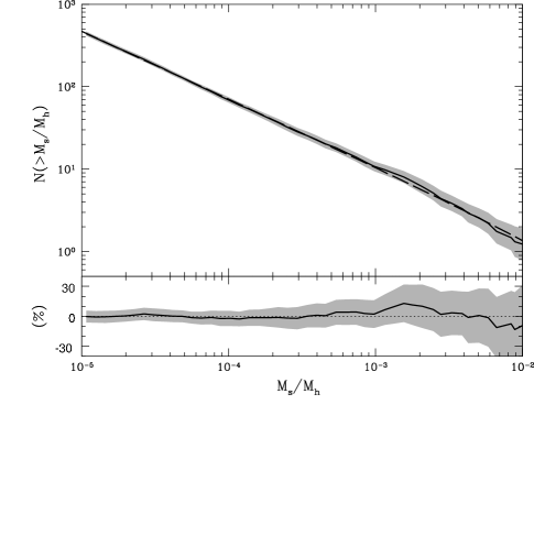
Figure 3.— Solid line: Number of subhalos found within the $10^{15}{h^{-1}M_{\odot}}$ halo at $z=0$ with a mass fraction above a value $M_{s}/M_{h}$, obtained in our model from the average of 10 numerical realizations. Shaded region: statistical uncertainty, computed from the error on the mean of the ten realizations. Dashed line: Analytic subhalo mass function found to fit results of full numerical simulations of halo substructure (Vale & Ostriker, 2006). Bottom panel: Percentage deviation of our calculation relative to this fit.

Figure 4.— Populating halos with black holes at $z=2$. $(a)$ Assumed relation of the halo and black hole masses, determined from their cumulative global mass functions at $z=2$. As an example, black holes of mass $\sim 6\times 10^{8}M_{\odot}$ are placed in halos of mass $\sim 10^{13}{h^{-1}M_{\odot}}$ by matching their cumulative number densities. $(b)$ Solid curve: black hole mass function in the cluster region at $z=2$; dashed curve: global black hole mass function at $z=2$.

4. Numerical Model

4.1. Merger Tree

We use the extended Press-Schechter formalism described in § 2.1 to generate the mass accretion histories of halos. We adopt a flat $\Lambda$CDM cosmology where the present Hubble constant is $h\equiv H_{0}/(100~{}{\rm km\,s}^{-1}{\rm Mpc}^{-1})=0.7$, the matter density is $\Omega_{m}=0.3$, the baryon density is $\Omega_{b}=0.02h^{-2}$, the power spectrum normalization is determined by $\sigma_{8}=0.9$, and the primordial spectral index is $n=1$ (e.g., Spergel et al. 2003; Tegmark et al. 2004). The power spectrum shape is obtained using the transfer function of Eisenstein & Hu (1999).

We are particularly interested in this paper in studying the origin of black holes (and the contribution of mergers to their growth) in massive galaxy clusters, such as the Coma cluster. We therefore generate a merger tree starting at $z=0$ with a halo mass $M_{\rm h}=10^{15}{h^{-1}M_{\odot}}$, and identify all the progenitor halos with mass larger than the mass resolution $M_{\rm res}$. In order to accurately follow the growth and accretion history of halos with masses near $M_{\rm res}$, we actually generate the merger tree down to a smaller mass, which for a halo of mass $M_{h1}$ is set to the minimum of $10^{-3}M_{h1}$ and $M_{\rm res}$. In this way, the variability of the halo mass growth due to the stochastic accretion of individual halos is adequately reproduced. However, only halos with mass above $M_{\rm res}$ are included when we follow their dynamical evolution and the history of their central black hole.

We adopt $M_{\rm res}=10^{10}{h^{-1}M_{\odot}}$ for the halos for which we follow the dynamical evolution. As we shall see in §5.1, the halos in which we place black holes in our model are of larger mass ($\gg 10^{11}{h^{-1}M_{\odot}}$) than our resolution limit, and the halos with no black holes are included in the calculation only for the purpose of taking into account the orbital perturbations they cause on the larger subhalos. We use a timestep for the merger tree corresponding to $\Delta z=10^{-4}$, which is small enough to ensure that $P\ll 1$ in equation (4). We have verified the validity of our Monte-Carlo procedure by generating many merger trees for a large number of halos with the $z=0$ Press-Schechter mass function, and comparing the obtained mass functions at high redshift to the analytic Press-Schechter mass function.

The halo mass function at $z=2$ for a high-density region that is constrained to assemble into a halo of mass $M_{\rm h}=10^{15}{h^{-1}M_{\odot}}$ at $z=0$ is shown in Figure 1 (solid line), compared to the globally averaged halo mass function at $z=2$ (dashed line). Hereafter, we use the term “globally averaged” to refer to a halo mass functions averaged over the whole universe, without any restrictions to regions with special properties. As expected, massive halos are more abundant than average in a region selected for forming a massive cluster at a later epoch. The average of ten different realizations of a merger tree was used for the statistical results presented below in Figures 3 and 7.

4.2. Examples of Dynamical Evolution

It is useful to illustrate with a few examples the way that the dynamical processes described in § 3 work to determine the evolution of the subhalos, and ultimately the merger rates of black holes in our model. Figure 2 plots the redshift-evolution of the pericenter ($r_{p}$), apocenter ($r_{A}$), Jaffe radius ($R_{s}$), and mass of six subhalos with black holes, which we have selected as illustrative examples (not randomly) from the merger tree for the formation of a halo with mass $M_{\rm h}=10^{15}{h^{-1}M_{\odot}}$ at $z=0$. We generally refer to the largest halo present in the merger tree as the “cluster halo.”

In our model, a halo grows in mass from accretion and mergers as long as it merges only with objects smaller than itself, and it becomes a subhalo when it merges into a larger object. From that point on, the mass of the subhalo can only decrease as it experiences tidal disruption. In Figures 2$a$ and 2$b$, the masses and radii of the subhalos are shown starting at the time they merge into the cluster halo. The decrease in mass and radius occurs at each pericenter passage, according to equation (21). The thick solid and long dashed lines in Figure 2$a$ show the mass of the cluster halo and of the central black hole, while the radius of the cluster halo is shown as the thick solid line in the other three panels.

The evolution of the orbits is shown in Figures 2$c$ and 2$d$, which plot the pericenter and apocenter as a function of time. There is an average tendency for the orbits to shrink because of dynamical friction. The rate at which the orbits shrink increases with subhalo mass and with proximity to the center. As the subhalos approach the center, their masses and radii are reduced by tidal disruption. It should be noted here that when the mass of both the subhalo and cluster halo inside radius $r$ vary linearly with $r$ (as is the case for Jaffe spheres in the inner parts), the mass of a subhalo after tidal disruption at pericenter $r_{p}$ will be proportional to $r_{p}$, and the ratio of the subhalo mass to the cluster halo mass enclosed within the subhalo orbit remains constant. Therefore, the ratio of the dynamical friction time to the orbital time remains constant also, and the subhalo continues to spiral toward the center in a constant number of orbits in each logarithmic radial interval. The subhalo is therefore completely destroyed in a finite time, and the black holes are then assumed to merge. In the example in the figures, two halos are destroyed in the center at $z\simeq 0.56$ and $z\simeq 0.25$, causing the jumps in the mass of the central black hole. The mass ratios of the two mergers are 30% and 83%, respectively. There is one more black hole that merges at $z\simeq 0.16$ with a mass ratio of 168% (not shown in the Figure for the sake of clarity). Another four halos are shown which are gradually decreasing their orbital radius but still survive by $z=0$. The halos added to the cluster at $z\simeq 0.25-0.3$ have a very slow rate of orbital decay, and their pericenter is large enough to avoid any tidal disruption. Their apocenters and pericenters show random variations owing to the gravitational encounters among subhalos.

In general, subhalos are destroyed when the dynamical friction time is shorter than the age of the system. Subhalos that avoid tidal disruption have an initial dynamical friction time long compared to the age of the universe. If the cluster halo were to remain perfectly static, eventually all subhalos would spiral to the center given a sufficiently long time. However, this does not happen because as the cluster halo continues to grow in mass, large subhalos that are continuously merging cause random perturbations on the orbits of smaller subhalos which can increase their orbital radii and therefore their dynamical friction times. Additionally, whenever the halo within which a satellite is orbiting merges into a larger system and is tidally disrupted, the satellite is placed in an orbit in the larger system with a much longer dynamical friction time. In this way, small subhalos can survive indefinitely orbiting in larger halos as long as the halos continue to merge and grow.

The important dynamical effects determining the rate of black hole mergers obtained in our model are the fraction of satellites that can spiral all the way into the center of their parent halo by dynamical friction before they are scattered, and the rate at which they are tidally disrupted as they pass near the halo center. Hence, the black hole merger rates we present in §6 are most sensitive to the rate of dynamical friction and mass loss by tidal disruption as a function of orbital eccentricity and semimajor axis, as well as the rate of orbital perturbations by other satellites.

As a test of our analytic model, we compare the subhalo mass function we obtain in the cluster halo at $z=0$, plotted in Figure 3, with results that have been obtained from numerical simulations. We include only subhalos on orbits with a circular radius smaller than the cluster halo radius, to compare with numerical simulation results where subhalos are identified as bound objects inside the virial radius of the parent halo. Our subhalo mass function is computed from the average of ten realizations of the merger tree of the cluster halo. We fit the result to a Schechter mass function for the subhalo mass function,

$$N(M_{s}|M_{\rm h})dM_{s}=A\left({M_{s}\over\beta M_{\rm h}}\right)^{-\alpha}\exp\left(-{M_{s}\over\beta M_{\rm h}}\right){dM_{s}\over\beta M_{\rm h}},\vspace{10pt}$$ (25)

where $\alpha$ is the power-law slope and $\beta M_{\rm h}$ is the cutoff mass (Vale & Ostriker, 2006). The normalization is given by

$$A={\gamma/\beta\over\Gamma[2-\alpha]-\Gamma[2-\alpha,M_{s,{\rm max}}/\beta M_{\rm h}]}~{},\vspace{10pt}$$ (26)

where the total mass fraction in subhalos is $\gamma$, $M_{s,{\rm max}}=0.5M_{\rm h}$ is the maximum subhalo mass, and $\Gamma[x]$ and $\Gamma[a,x]$ are the Gamma and the incomplete Gamma functions, respectively. We fix the cutoff mass fraction to $\beta=0.3$ (Shaw et al., 2005) and fit the analytic function to our results, allowing the parameters $\alpha$ and $\gamma$ to vary. The resulting best-fit subhalo mass function is shown as a dashed line, and has values $\alpha=1.82$ and $\gamma=0.12$, in good agreement with typical values found in numerical simulations, $\alpha=1.7-1.9$ and $\gamma\simeq 0.1$ (De Lucia et al., 2004; Shaw et al., 2005; Zentner et al., 2005). Our model basically agrees with the results found in simulations within the uncertainty.

5. Black Hole Mass Function in Clusters at $z=2$

This section describes the way we initially populate halos with central black holes. Our dynamical evolution model described previously tells us the rate at which halos merge all the way to their central cusps, and we assume that the merger of the central black holes follows immediately after the merger. The simple model that we now describe for the initial population of black holes in halos allows us to derive a rate of black hole mergers from the rate of halo mergers that proceed all the way to their centers.

A full model of the evolution of the black hole mass function including the effects of gas accretion and mergers would include the gradual growth of black holes from gas accretion as constrained by observations of the quasar luminosity function at each redshift, and would simultaneously follow black hole mergers from the dynamical evolution of host halos. Here we make a simplifying assumption that separates the two evolutionary factors for the growth of black holes: gas accretion and mergers. Observationally, we know that most of the radiative energy of luminous quasars was emitted over a narrow range of redshift, $1.5\lesssim z\lesssim 4$ (e.g., Croom et al., 2004; Richards et al., 2006). Hence, we make the approximation that gas accretion creates all the black holes instantaneously at $z=2$, roughly at the epoch of the peak in quasar activity, and that subsequently the black hole mass function evolves only by mergers. We choose to place the black holes in halos at $z=2$ with their observed mass function at $z=0$. If black hole mergers cause relatively small changes in the black hole mass distribution, then the evolved mass function should still be approximately correct.

The black hole mass function at $z=0$ is often estimated by using observed luminosity functions or velocity dispersion measurements of galaxies, and observed correlations with the central black hole masses. Here we use the black hole mass function obtained by Steed & Weinberg (2003). This is derived from the distribution of early-type galaxy velocity dispersions (Sheth et al., 2003) using the relation between the black hole mass $M_{\bullet}$ and velocity dispersion $\sigma$ in Tremaine et al. (2002), and adding also a contribution from spiral galaxies (these become the dominant host galaxies of black holes with $M_{\bullet}\leq 10^{8}M_{\odot}$, using the estimate of Aller & Richstone (2002) ). We also include an intrinsic scatter to the $M_{\bullet}-\sigma$ power-law relation of 0.5 dex, with a log-normal distribution in black hole mass.

We assign black holes to host halos at $z=2$ by assuming that all halos that have not merged into any larger object contain a black hole by $z=2$, and that there is a monotonically increasing, one-to-one relation between the halo mass, $M_{\rm h}$, and the corresponding black hole mass, $M_{\bullet}(M_{\rm h})$, at this redshift. This implies that the cumulative number densities of halos with mass above $M_{\rm h}$ must be equal to the cumulative number density of black holes with mass above $M_{\bullet}(M_{\rm h})$. This is illustrated in Figure 4$a$, where the globally averaged halo and black hole mass functions are plotted. As an example, halos of mass $M_{\rm h}=10^{13}{h^{-1}M_{\odot}}$ have the same number density as black holes of mass $6\times 10^{8}M_{\odot}$, so we place a black hole of this mass in each halo of mass $M_{\rm h}$. We apply this relation down to a minimum black hole mass of $10^{6}M_{\odot}$, which corresponds to a halo mass $M_{\rm h}\geq 8\times 10^{11}{h^{-1}M_{\odot}}$.

Note that the merger tree and the dynamical evolution of halos are computed from $z\gg 2$, even though black holes are only assigned to halos at $z=2$. Furthermore, the black holes have $no$ impact on the dynamical evolution of their host halos in our model. When orbiting halos merge all the way to their centers, we simply add the mass of their two black holes to obtain the mass of the new central black hole.

In Figure 4$b$, the black hole mass function in the cluster halo at $z=2$ obtained in this way is compared to the globally averaged black hole mass function. The black hole mass function in the cluster halo that we simulate is of course not the same as the globally averaged black hole mass function because, owing to the biased spatial distribution of halos, the region that collapses into a massive halo at $z=0$ contains an excess density of halos at $z=2$ and therefore an excess density of black holes compared to the global average. The mass function is shown as the number of black holes per unit of comoving original volume before the cluster collapses. Therefore the larger number density of black holes is not due to the physical collapse of the cluster halo, and reflects only the biased distribution of black holes.

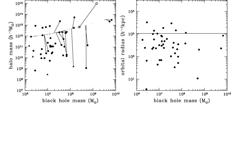
Figure 5.— Distribution of satellite halos containing a nuclear black hole in one realization of the cluster halo. Left panel: Filled symbols indicate masses of black holes and their host subhalos at $z=0$. Small dots give the initial relation between halo mass and black hole mass at $z=2$. For black holes that have merged, the initial and final masses are connected; for other black holes, only the halo masses have changed. The asterisk and open circle identify the central halo and black hole in the cluster. Squares indicate subhalos that have their own satellite halos with black holes, and these satellites are shown as triangles. Right panel: Orbital radius of satellites hosting a black hole in the cluster (the central black hole is not plotted). The horizontal bar is the radius of the cluster.

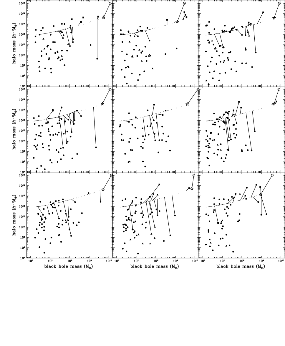
Figure 6.— Distribution of the black holes in the nine additional realizations of the merger tree of the cluster halo. The symbols are the same as Fig. 5.

Figure 7.— $(a)$ Thin solid lines: Halo mass function in the $M=10^{15}{h^{-1}M_{\odot}}$ cluster at $z=0$ in each realization. Thick solid: Halo mass function averaged over the ten realizations. Thick dashed: Globally averaged halo mass function. $(b)$ Black hole mass function in the cluster initially (at $z=2$) and at $z=0$, after the mergers have occurred. The thick dashed line is the globally averaged black hole mass function. $(c)$ and $(d)$ Individual small dots are the number of mergers and mass growth factors for black holes that have merged in ten realizations. Thick solid lines are averages. Thin solid lines are the number of mergers and mass ratios, when interaction between subhalos is ignored.

6. Impact of Mergers on Black Hole Growth

In this section, we present the results on the impact of mergers on the black hole mass function in a massive cluster and the way black holes are distributed in a cluster. We do not consider any possible ejections of black holes due to gravitational wave recoil, and we neglect the mass lost due to the emission of gravitational waves during mergers.

First, we examine the results of one particular realization of a $10^{15}{h^{-1}M_{\odot}}$ halo. The left panel in Figure 5 shows the initial and final values of the black hole mass and the host subhalo mass for all the black holes hosted by satellite halos of the cluster. The small dots are the values at $z=2$, and they follow the black hole mass$-$halo mass relation that we impose as initial conditions. At $z=0$, the black hole and halo masses are shown as filled symbols. The central black hole in the cluster is the one hosted by the main halo with mass $10^{15}{h^{-1}M_{\odot}}$, and all other halos have become satellites in the cluster. Subhalos with their own satellite systems that have survived tidal disruption by the main cluster halo are shown as filled squares, and satellites of subhalos are shown as triangles. Note that the evolution of the halos from $z=2$ to $z=0$ may either increase the halo mass due to mergers and accretion of other halos, or decrease the halo mass due to tidal stripping and disruption when they become subhalos in a larger halo. On the other hand, the black hole mass can only increase if two black holes merge, following a complete disruption of the host subhalo. To facilitate the identification of progenitor black holes, we connect filled symbols ($z=0$) and dots ($z=2$) of the black holes that have experienced any mergers. The right panel in Figure 5 shows the final orbital radius of each satellite in the cluster and the black hole mass, showing little correlation between these two quantities, except perhaps at the highest masses where the black holes may tend to be hosted by satellites closer to the cluster center.

Most of the black holes with masses above $\sim 10^{7.5}M_{\odot}$ experience mergers, and some of them increase their mass in a substantial way. The central black hole is the one that grows the most, experiencing many mergers and growing its mass by a factor $\sim 5$. At lower masses, most black holes do not experience any merger; for these, the filled symbol is at the same black hole mass as the small dot (note that some small dots do not have any corresponding large symbol because they have merged with a more massive black hole). In our dynamical model, the satellites representing the host galaxies of these black holes form galaxy groups and later become part of a larger cluster, where their dynamical friction time is too long to produce any significant decay. Although the outer parts of these satellites may be tidally disrupted (producing the large reductions in halo mass for most of the cases shown in the figure), the core of the satellite containing the black hole survives and remains as a satellite halo. We need to caution that the rarity of mergers for low-mass black holes may be caused in our model by the fact that we do not include black holes with initial mass below $10^{6}M_{\odot}$, and we place all the black holes at $z=2$ in field halos (halos that are not satellites in a larger halo).

The black hole that ends up in the cluster center is identified as the one that was present in the original halo which, merging only with other halos smaller than itself, became the cluster halo at $z=0$. In any merger-tree simulation of the formation of a cluster, there is one and only one initial halo that has always merged with other halos smaller than itself, which is found by tracing back the merger history from the final cluster and choosing always the most massive progenitor halo at every merger event. This halo is not necessarily the most massive halo at $z=2$. Because the growth rates of halos are stochastic, there may be halos of high mass at $z=2$ which grow slowly, while other halos of originally lower mass grow faster and become more massive by the time that all the halos merge to form the final cluster at $z=0$. This is in fact the case in the example of Figure 5, where the initial halo that becomes the center of the final cluster is identified by an asterisk. This central progenitor has a mass of $\sim 10^{12.7}{h^{-1}M_{\odot}}$ at $z=2$ and it grows rapidly to become the cluster halo, while several other halos that were originally more massive (the largest having nearly $10^{14}{h^{-1}M_{\odot}}$ at $z=2$) become satellites as they merge at late times with the fast-growing halo. When this situation occurs, the black hole in the central galaxy will not be the most massive one. In the present example, the black hole in the cluster center would have a mass of only $10^{9.2}M_{\odot}$, while black holes in other satellite galaxies have masses as high as $\sim 10^{9.8}M_{\odot}$.

This situation, however, is not the most common one, as can be seen in Figure 6, where an additional nine random realizations of the formation of a $10^{15}{h^{-1}M_{\odot}}$ halo are examined. In the majority of cases, the halo that becomes the final cluster at $z=0$ was the most massive halo at $z=2$. Out of the ten random realizations we have performed, there is only one case where black holes in satellite galaxies are substantially more massive than the black hole ending up at the center, but there are several where black holes in satellite galaxies are of comparable mass to the central one. We also see that there is a substantial dispersion for the mass of the central black hole in a cluster of fixed mass ($10^{15}{h^{-1}M_{\odot}}$), going from values as high as $1.5\times 10^{10}M_{\odot}$ to as low as $2\times 10^{9}M_{\odot}$. If we take the most massive black hole in the cluster (rather than the central one), then the low-end of this mass range increases to $4\times 10^{9}M_{\odot}$, still implying a substantial dispersion.

In practice, the distinction between the black hole in the cluster center and black holes in satellites is ambiguous observationally. Clusters typically have substructure and may have more than one galaxy that could qualify as “central.” However, observationally we know that there is a linear correlation between black hole mass and the stellar mass of an elliptical galaxy (or the bulge component of a spiral galaxy). This observed relation tells us that, irrespective of whether a giant galaxy is considered to be the central one in a cluster or a satellite, its stellar mass should follow the same correlation with black hole mass that was imprinted during the quasar epoch at high redshift. Mergers will increase the mass of a black hole and the spheroidal stellar component by the same factor (neglecting gravitational wave emission and ejected stars), so in any clusters where the central black hole is not the most massive one, it should probably also be true that the central galaxy is not the one with the largest stellar mass, and that the most massive black hole is in the galaxy with the most massive stellar component.

Figure 7 summarizes the results of the ten realizations. The initial halo mass functions at $z=2$ of the ten realizations are shown in the first panel, together with the average mass function. The mass functions in the realizations contain many more massive halos than average because of the bias introduced when selecting a region that forms a $10^{15}{h^{-1}M_{\odot}}$ halo at $z=0$. The second panel shows the black hole mass functions. For the same reason, the initial mass function contains many more massive black holes per unit volume than the average mass function. Black hole mergers result in a substantial change in the black hole mass function, in particular a large increase in the number of black holes of $M\gtrsim 5\times 10^{9}M_{\odot}$.

Because of this increase, our initial conditions in which the $z=2$ black hole mass function matches the $z=0$ mass function are not fully consistent with our results. However, one should note that Figure 7$b$ shows the change in the black hole mass function in a $10^{15}{h^{-1}M_{\odot}}$ cluster, and that such clusters are rare; the global evolution of the high end of the mass function will be weaker.

In the last two panels, thick solid histograms show the number of mergers experienced by each black hole in terms of the black hole mass, and the average factor by which the black hole mass increases as a result of these black hole mergers. Figure 6c shows that most black holes of $M\gtrsim 10^{8}M_{\odot}$ experience mergers. However, their mass growth is small except for the most extremely massive black holes, $M\gtrsim 3\times 10^{9}M_{\odot}$. The majority of black holes, with lower masses, grow only by a small factor because they often merge with black holes of much lower mass than themselves. At low masses, black holes are removed by merging into more massive objects, causing a decrease in the mass function of a factor of $\sim 2$ (Fig.7$b$). We are cautious in interpreting this result because it may be severely affected by our approximation of placing the black holes initially at $z=2$: had we followed the evolution of black holes from a higher redshift, when many more low-mass halos are present, many more mergers of low-mass halos (and their central low-mass black holes) would probably have occurred. The minimum black hole mass of $10^{6}M_{\odot}$ in our simulation should probably also be increased in order to correctly follow the black hole mergers at higher redshift, and a model of black hole growth from gas accretion that is distributed over redshift (instead of occurring instantaneously at $z=2$, as we have assumed here) would need to be included.

A fundamental process affecting the way black hole mergers can occur in our model is the mechanism of random orbital perturbations described in § 3.5 to take into account the interactions of the satellite halo containing the black hole with other satellites. If these perturbations are absent, a satellite can only continue to undergo orbital decay by dynamical friction, unless its parent halo merges into another object. The perturbations allow a satellite to randomly gain orbital energy and in this way avoid tidal destruction. It is therefore useful to check how much our merger rates are altered if we suppress these interactions, to see if the results are highly sensitive to their presence and to the detailed way in which we implement the perturbations. This is quantified in Figure 7, in panels ($c$) and ($d$), where thin solid histograms show the results with the perturbations turned off. As expected, the number of black hole mergers increases, although by a relatively small amount, while the mass growth remains similar. Hence the results are not greatly affected by the presence of the perturbations. We also find that the enhanced disruption of subhalos when perturbations are turned off results in a subhalo mass function for which only 7% of the total mass is contained in subhalos, less than is found in numerical simulations. Thus, our physically motivated recipe for including orbital perturbations produces better agreement between the analytic model and numerical simulations (see Fig.3).

7. Conclusions

We have developed a dynamical model of substructure in dark matter halos based on numerical merger trees and analytic models of the dynamical evolution of satellites, with the purpose of modeling the rates of mergers of nuclear black holes. We have improved on previous work by tracing the evolution of satellites in a satellite halo, and by accounting for satellite-satellite interactions. Our model reproduces the analytic subhalo mass function found previously in numerical simulations, for $M_{s}\geq 10^{-5}M_{\rm h}$ in a halo of $M_{\rm h}=10^{15}{h^{-1}M_{\odot}}$. In this paper, we have focused on examining the effect of mergers on the abundances of the most massive black holes in clusters of galaxies, using a simplified model where black holes have completed their growth by gas accretion by $z=2$ and remain with a fixed mass after that, unless they undergo mergers when their host galaxies merge. We have assumed that the merger of two satellites in a halo always leads to the merger of their central black holes (which maximizes the merging rate for black holes).

We find that mergers have an important impact on the most massive black holes in the cluster. For the most massive black holes in a cluster, with $M>10^{9}M_{\odot}$, a growth in mass by a factor $\sim 2$ is typical. Our ten realizations of a $10^{15}{h^{-1}M_{\odot}}$ cluster include four black holes with a final mass of $1-1.5\times 10^{10}M_{\odot}$, but without mergers such black holes would be extremely rare.

Mergers are less important for black holes of lower mass. The main effect found in our simulation on low-mass black holes is that they are depleted by a factor $\sim 2$ because of their mergers into more massive black holes. This result may be affected by our procedure of initially populating the halos with black holes at $z=2$, and by the minimum black hole mass of $10^{6}M_{\odot}$ that we use. We also caution that the effect of depletion in the global black hole mass function may be much weaker than the effect in the cluster environment, because by the epoch of $z=2$, most of the low-mass black holes that were formed in a region collapsing in a massive cluster at present have already merged in larger objects.

We have also found that the most massive black hole is not always located in the central galaxy of the cluster, if we define the central galaxy to be the one that formed in the halo that has always merged with other halos smaller than itself. In practice, it may be difficult to assign observationally which galaxy in the cluster corresponds to this central one; moreover, the linear relation between black hole mass and bulge stellar mass should not be altered.

Our model may overestimate the importance of mergers because we have assumed that, once the nuclei of two satellite halos have approached each other down to the radii of influence of the black holes, the black holes will always merge. Actually, two black holes may become stalled after they have scattered all the stars interior to their orbit as well as any remaining stars in the loss-cone, and before reaching the radius of orbital decay by gravitational waves (Begelman, Rees & Blandford, 2006), so it may be that not all black hole binaries merge. It is unlikely that a majority of mergers end up in stalled binary systems, however, because few binary black holes in galactic nuclei are found, and because the presence of gas is likely to drive the binary to a merger in any case (Gould & Rix 2000). Moreover, models that try to estimate the probability of ejection of black holes during three-body interactions find that only a small fraction of the black holes can be lost in this way (Volonteri et al. 2003).

Therefore, the results of our paper support the idea that black hole mergers are important in shaping the black hole mass function at low $z$, particularly affecting in a strong way the abundance of the most massive black holes in rich clusters of galaxies. In a subsequent paper, we shall examine more generally the impact of mergers on the evolution of black holes outside of massive clusters.

References

- Aller & Richstone (2002) Aller, M. C., & Richstone, D. 2002, AJ, 124, 3035
- Barger et al. (2001) Barger, A. J., Cowie, L. L., Bautz, M. W., Brandt, W. N., Garmire, G. P., Hornschemeier, A. E., Ivison, R. J., & Owen, F. N. 2001, AJ, 122, 2177
- Begelman, Rees & Blandford (2006) Begelman, M. C., & Rees, M. J., & Blandford, R. D. 1980, Nat, 287, 307
- Begelman, Volonteri & Rees (2006) Begelman, M. C., Volonteri, M., & Rees, M. J. 2006, MNRAS, 370, 289
- Binney & Tremaine (1987) Binney, J., & Tremaine, S. 1987, Galactic Dynamics (Princeton: Princeton Univ. Press)
- Bond et al. (1991) Bond, J. R., Cole, S., Efstathiou, G., & Kaiser, N. 1991, ApJ, 379, 440
- Bryan & Norman (1998) Bryan, G. L., & Norman, M. L. 1998, ApJ, 495, 80
- Bullock, Kravtsov & Weinberg (2000) Bullock, J. S., Kravtsov, A. V., & Weinberg, D. H. 2000, ApJ, 539, 517
- Bullock, Kravtsov & Weinberg (2001) Bullock, J. S., Kravtsov, A. V., & Weinberg, D. H. 2001, ApJ, 548, 33
- Carroll, Press & Turner (1992) Carroll, S. M., Press, W. H., & Turner, E. L. 1992, ARA&A, 30, 499
- Cole et al. (2000) Cole, S., Lacey, C. G., Baugh, C. M., & Frenk, C. S. 2000, MNRAS, 319, 168
- Croom et al. (2004) Croom, S. M., Smith, R. J., Boyle, B. J., Shanks, T., Miller, L., Outram, P. J., & Loaring, N. S. 2004, MNRAS, 349, 1397
- De Lucia et al. (2004) De Lucia, G., et al. 2004, MNRAS, 348, 333
- Eisenstein & Hu (1999) Eisenstein, D. J., & Hu, W. 1999, ApJ, 511, 5
- Eke, Cole & Frenk (1996) Eke, V. R., Cole, S., & Frenk, C. S. 1996, MNRAS, 282, 263
- Fan et al. (2003) Fan, X. et al. 2003, AJ, 125, 1649
- Ferrarese & Merritt (2000) Ferrarese, L., & Merritt, D. 2000, ApJ, 539, 9L
- Fukushige & Makino (2001) Fukushige, T., & Makino, J. 2001, ApJ, 557, 533
- Gebhardt et al. (2000) Gebhardt, K., et al. 2000, ApJ, 539, 13L
- Gnedin (2003) Gnedin, O. Y. 2003, ApJ, 582, 141
- Gould Rix (2000) Gould, A., & Rix, H.-W. 2000, ApJ, 532, 29
- Hayashi et al. (2003) Hayashi, E., Navarro, J. F., Taylor, J. E., Stadel, J., & Quinn, T. 2003, ApJ, 584, 541
- Jaffe (1983) Jaffe, W. 1983, MNRAS, 202, 995
- Jenkins et al. (2001) Jenkins, A., Frenk, C. S., White, S. D. M., Colberg, J. M., Cole, S., Evrard, A. E., Couchman, H. M. P., & Yohida, N. 2001, MNRAS, 321, 372
- Lacey & Cole (1993) Lacey, C., & Cole, S. 1993, MNRAS, 262, 627
- Lynden-Bell (1969) Lynden-Bell, D. 1969, Nature, 223, 690
- Magorrian et al. (1998) Magorrian, J., et al. 1998, AJ, 115, 2285
- Moore et al. (1999) Moore, B., Quinn, T., Governato, F., Stadel, J., & Lake, G. 1999, MNRAS, 310, 1147
- Navarro, Frenk & White (1997) Navarro, J. F., Frenk, C. S., & White, S. D. M. 1997, ApJ, 490, 493
- Navarro et al. (2004) Navarro, J. F., et al. 2004, MNRAS, 349, 1039
- Press & Schechter (1974) Press, W. H., & Schechter, P. 1974, ApJ, 187, 425
- Richards et al. (2006) Richards, G. T., et al. 2006, AJ, 131, 2766
- Salpeter (1964) Salpeter, E. E. 1964, ApJ, 140, 796
- Shankar et al. (2006) Shankar, F., Lapi, A., Salucci, P., De Zotti, G., & Danese, L. 2006, ApJ, 643, 14
- Shaw et al. (2005) Shaw, L., Weller, J., Ostriker, J. P., & Bode, P. 2006, ApJ, 646, 815
- Sheth et al. (2003) Sheth, R. K., et al. 2003, ApJ, 594, 225
- Sheth & Tormen (1999) Sheth, R. K., & Tormen, G. 1999, MNRAS, 308, 119
- Sołtan (1982) Sołtan, A. 1982, MNRAS, 200, 115
- Spergel et al. (2003) Spergel, D. N. et al. 2003, ApJS, 148, 175
- Steed & Weinberg (2003) Steed, A., & Weinberg, D. H. 2003, ApJ, submitted (astro-ph/0311312)
- Taffoni et al. (2003) Taffoni, G., Mayer, L., Colpi, M., & Governato, F. 2003, MNRAS, 341, 434
- Taylor & Babul (2001) Taylor, J. E., & Babul, A. 2001, ApJ, 559, 716
- Taylor & Babul (2003) Taylor, J. E., & Babul, A. 2004, MNRAS, 348, 811
- Tegmark et al. (2004) Tegmark, M., et al. 2004, Phys. Rev. D, 69, 103501
- Tormen, Diaferio & Syer (1998) Tormen, G., Diaferio, A., & Syer, D. 1998, MNRAS, 299, 728
- Tremaine et al. (2002) Tremaine, S., et al. 2002, ApJ, 574, 740
- Vale & Ostriker (2006) Vale, A., & Ostriker, J. P. 2006, MNRAS, 371, 1173
- Volonteri, Haardt & Madau (2003) Volonteri, M., Haardt, F., & Madau, P. 2003, ApJ, 582, 559
- Yu & Tremaine (2002) Yu, Q., & Tremaine, S. 2002, MNRAS, 335, 965
- Zel’dovich & Novikov (1964) Zel’dovich, Y. B., & Novikov, I. D. 1964, Dokl. Akad. Nauk. SSSR, 158, 811 (English translation: 1965, Sov. Phys. Dokl., 9, 834)
- Zentner & Bullock (2003) Zentner, A. R., & Bullock, J. S. 2003, ApJ, 598, 49
- Zentner et al. (2005) Zentner, A. R., Berlind, A. A., Bullock, J. S., Kravtsov, A. V., & Wechsler, R. H. 2005, ApJ, 624, 505