Gaussian decomposition of H i surveys

Abstract

Context. To investigate the properties of the 21-cm radio-lines of galactic neutral hydrogen, the profiles of “The Leiden/Argentine/Bonn (LAB) Survey of Galactic H i” are decomposed into Gaussian components.

Aims. The width distribution of the obtained components is analysed and compared with similar studies by other authors.

Methods. The study is based on an automatic profile decomposition algorithm. As the Gaussians obtained for the complex H i profiles near the galactic plane cannot be directly interpreted in terms of the properties of gas clouds, we mainly study the selected simplest profiles in a limited velocity range. The selection criteria are described and their influence on the results is discussed.

Results. Considering only the simplest H i profiles, we demonstrate that for Gaussians with relatively small LSR velocities ($-9\leq V_{\mathrm{C}}\leq 4\leavevmode\nobreak\ \mathrm{km\,s}^{-1}$) it is possible to distinguish three or four groups of preferred line-widths. The mean widths of these groups are $\mathrm{FWHM}=3.9\pm 0.6$, $11.8\pm 0.5$, $24.1\pm 0.6$, and $42\pm 5\leavevmode\nobreak\ \mathrm{km\,s}^{-1}$. Verschuur previously proposed similar line-width regimes, but with somewhat larger widths. He used a human-assisted decomposition for a nearly 50 times smaller database and we discuss systematic differences in analysis and results.

Conclusions. The line-widths of about 3.9 and $24.1\leavevmode\nobreak\ \mathrm{km\,s}^{-1}$ are well understood in the framework of traditional models of the two-phase interstellar medium. The components with the widths around $11.8\leavevmode\nobreak\ \mathrm{km\,s}^{-1}$ indicate that a considerable fraction (up to about 40%) of the H i gas is thermally unstable. The reality and the origin of the broad lines with the widths of about $42\leavevmode\nobreak\ \mathrm{km\,s}^{-1}$ is more obscure. These, however, contain only about 4% of the total observed column densities.

1 Introduction

The tradition to analyse the 21-cm H i line profiles in terms of Gaussian components has its roots in the finding that the H i absorption features are often well represented by Gaussian functions in optical depth $\tau(\nu)$. This is understandable when the line profile is dominated by the thermal motions or nonthermal motions consisting of a large number of turbulent elements. The decomposition of the emission profiles is physically meaningful only when $\tau(\nu)\ll 1$. Nevertheless, both the opacity and brightness profiles of most sources are easily decomposed into Gaussains, so whether or not this model is physically correct, it works empirically and is convenient. Moreover, even if such a decomposition is not a physically valid description of the galactic ISM, it is a valid mathematical description of the corresponding 21-cm H i profile.

Mathematically the most questionable point of the Gaussian decomposition is that often it is not unique. This nonuniqueness means that several quite different solutions may approximate the observed profile almost equally well, and the decomposition provides no satisfactory means for choosing between these solutions, while others, equally good or even better ones, may not be found at all. However, when we decompose a large number of profiles by exactly the same algorithm, we may hope that for similar profiles the algorithm will prefer similar decompositions. This means that usually some specific features in the observed profiles are represented by some specific set of Gaussians, which can be found from the overall data-set more easily than un-parametrized spectral features. The latter is one of our main interests in Gaussian decomposition and from this point of view all obtained Gaussians are real, as they describe some features in observed profiles. If and how these Gaussians are related to the physical properties of the galactic ISM is a question, which must be answered separately for every selected subset of the components.

Proceeding from these considerations, in the first paper of this series (Haud Hau00 (2000), hereafter Paper I) we described a new fully automated computer programme for the decomposition of large 21-cm H i line surveys into Gaussian components. We used the Leiden/Dwingeloo Survey (LDS) of galactic neutral hydrogen (Hartmann Har94 (1994)) as test data for decomposition. After our initial paper a new revision of the LDS data (LDS2) has been published (Kalberla et al. Kal05 (2005)). Recently a similar Southern sky high sensitivity H i survey at $\delta\leq-25\degr$ was completed in the Instituto Argentino de Radioastronomia (IARS) and published by Bajaja et al. (Baj05 (2005)). Both surveys have been combined to form the Leiden/Argentine/Bonn (LAB) full sky database (Kalberla et al Kal05 (2005)). Using our Gaussian decomposition programme, we have decomposed all profiles in these surveys.

The specifications for the LDS2 and the IARS closely match each other, but all the data reduction and calibration procedures for combining them into the LAB were carried out entirely independently (Kalberla et al. Kal05 (2005)). Proceeding from this, also the Gaussian decomposition was carried out separately for the LDS2 and the IARS. For the published version of the LDS2, in the cases of repeated observations at the same sky positions, the final profiles were selected on the basis of the best agreement of their preliminary Gaussian decompositions with the decompositions of the neighbouring profiles (Kalberla et al. Kal05 (2005)) and for our final decomposition we used these preselected profiles. In the case of the IARS, we used for the decomposition the original 1008-channel data of all the observed profiles and for repeated observations we applied before the final decomposition the same selection criteria as used for the LDS2.

In both surveys the observations were made on a galactic coordinate grid with observed points spaced by $(\Delta l,\Delta b)=(0\aas@@fstack{\circ}5/\cos b,0\aas@@fstack{\circ}5)$. The velocity resolution was $1.03\leavevmode\nobreak\ \mathrm{km\,s}^{-1}$ in the case of the LDS2 and $1.27\leavevmode\nobreak\ \mathrm{km\,s}^{-1}$ for the IARS. For both surveys the authors declare the final rms noise of the data to be about $0.07\leavevmode\nobreak\ \mathrm{K}$, but our estimates have given somewhat larger values. For the LDS we have obtained an estimate of $0.09\leavevmode\nobreak\ \mathrm{K}$ (Paper I) and the same value is given also by Westphalen (Wes97 (1997)). With the IARS the situation seems to be more complicated (Haud & Kalberla Hau06 (2006), hereafter Paper II). When for the signal-free regions of the profiles the estimate given by the authors of the survey seems to be correct, in the regions containing the emission signal, we estimated higher noise levels than it may be expected on the basis of the signal-free regions and the radiometer equation. From the regions containing the line emission we estimated the noise level for zero intensity line emission to be about $0.08\leavevmode\nobreak\ \mathrm{K}$ (Fig. 12. of Paper II).

When performing the Gaussian decomposition, the main attention was turned on keeping the number of resulting Gaussians as small as possible (Paper I). For every profile in the first decomposition stage new Gaussians were added until the rms of the residuals became less or equal to the noise level of the signal-free regions of the profile. The dependence of the noise level on the signal strength was taken into account according to the radiometer equation. After preliminary decomposition of each profile special analysis was applied to find additional possibilities for removing some less important components from the final decomposition without increasing the residuals above the noise level. To reduce the ambiguities in choosing between different, but nearly equally acceptable solutions, we have used the assumption that in survey observations the profiles from neighbouring sky positions must share some common properties and therefore their decompositions must be as similar as possible. The described procedure gave us 1 064 808 Gaussians per 138 830 profiles for the LDS2 and 444 573 Gaussians per 50 980 profiles in the case of the IARS.

In Paper II we analysed the distributions of the parameters of the obtained components. We discussed both the original LDS data and the newer LAB. The main attention was paid to the separation of the Gaussians describing different artefacts of the observations (interferences), reduction (baseline problems) and the decomposition (separation of the signal from the noise) process. In the present paper, we continue the analysis of the distribution of the Gaussian parameters, but in this case the main focus is on the components, most likely corresponding to the galactic H i. We start with the general distribution of all Gaussians and concentrate on the distribution of the widths of weak components with near zero velocities.

Earlier, a similar distribution has extensively been studied by Verschuur and co-authors (Ver89 (1989), Ver94 (1994), Ver99 (1999), Ver02 (2002), Ver04 (2004)). Their results are qualitatively very similar to ours, but we must note some differences in the quantitative values. By trying to follow the approach used by Verschuur, we point out the main differences found and their possible influence on the final results. In the concluding sections of the paper, we discuss the relation of our results to the properties of the galactic H i.

2 The general distribution of Gaussian widths

In Paper II we discussed mainly the frequency distribution of the Gaussians in their height vs. width plane (Fig. 1). We defined the height of a Gaussian by the value of the central brightness temperature $T_{\mathrm{b0}}>0$ from the standard Gaussian formula

$$T_{\mathrm{b}}=T_{\mathrm{b0}}\mathrm{e}^{-\frac{(V-V_{\mathrm{C}})^{2}}{2\sigma_{V}^{2}}},$$ (1)

where $T_{\mathrm{b}}$ is the brightness temperature and $V$ is the velocity of the gas relative to the Local Standard of Rest. $V_{\mathrm{C}}$ is the velocity corresponding to the centre of the Gaussian. We characterise the widths of the components by their full width at the level of half maximum ($\mathrm{FWHM}$), which is related to the velocity dispersion $\sigma_{V}$ obtained from our decomposition programme by a simple scaling relation $\mathrm{FWHM}=\sqrt{8\ln{2}}\sigma_{V}$.

In Paper II we have demonstrated that not all Gaussians obtained in our decomposition and represented in Fig. 1 could be considered as corresponding to the real H i emission. A considerable number of the obtained components are due to different observational, reductional and decompositional problems. Very narrow Gaussians actually represent the strongest random noise peaks misinterpreted by the decomposition programme as possible signal peaks and the radio-interferences not found or properly removed during the reduction of the observed profiles. Many of somewhat wider weak Gaussians seem to be caused by the increased uncertainties in bandpass removal near the profile edges. In the direction of even wider Gaussians, at least some weak components may be due to the problems in the determination of the profile baselines, but some of these Gaussians may also arise from the emission of the high velocity dispersion halo gas (HVDHG) reported by Kalberla et al. (Kal98 (1998)).

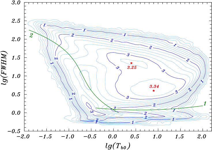
Figure 1: Frequency distribution of the parameter values in $(\lg(T_{\mathrm{b0}}),\lg(\mathrm{FWHM}))$ plane for all Gaussians obtained in the decomposition of the LAB. Isodensity lines are drawn in the scale of $\lg(N+1)$ with the interval of 0.2. The two main maxima are labelled with their height values. The green thick solid lines 1 and 2 represent the selection criteria discussed in Paper II.

In Fig. 1 such spurious components (in the lower left-hand part of the figure) are separated by two thick solid lines from the others (in the upper right-hand part of the figure) more likely describing the real galactic H i emission. However, from Fig. 1 we can also see that the parameters of the components, most likely corresponding to the galactic H i, are not distributed randomly, but exhibit concentration around two more or less distinct values. We can clearly see such a concentration around the values of $T_{\mathrm{b0}}\approx 8\leavevmode\nobreak\ \mathrm{K}$, $\mathrm{FWHM}\approx 4\leavevmode\nobreak\ \mathrm{km\,s}^{-1}$ and a weaker one at $T_{\mathrm{b0}}\approx 2.5\leavevmode\nobreak\ \mathrm{K}$, $\mathrm{FWHM}\approx 22\leavevmode\nobreak\ \mathrm{km\,s}^{-1}$. This finding is in general agreement with the earlier results by Mebold (Meb72 (1972)), who decomposed nearly 1700 21-cm H i emission line profiles into about 2400 Gaussian components and found that their width distribution has two distinct maxima at $\mathrm{FWHM}\approx 7\leavevmode\nobreak\ \mathrm{km\,s}^{-1}$, mostly populated by components with $10\la T_{\mathrm{b0}}\la 50\leavevmode\nobreak\ \mathrm{K}$ (narrow components), and $24\leavevmode\nobreak\ \mathrm{km\,s}^{-1}$ for Gaussians with $3\la T_{\mathrm{b0}}\la 10\leavevmode\nobreak\ \mathrm{K}$ (shallow components).

Mebold (Meb72 (1972)) used the profiles with lower spectral resolution than that of the LAB. Moreover, his profiles were from relatively low galactic latitudes and the stronger emission components become wider and more non-Gaussian due to the saturation and self-absorption. Considering this, we have a surprisingly good match of the maxima of at first glance physically meaningless (lumping into one high-latitude H i and heavily-saturated low-latitude galactic disk profiles, HVC’s and IVC’s and even the observational, reductional and decompositional artefacts) distribution in Fig. 1 with the ones described by Mebold. In his paper Mebold concluded: “… it is most likely that the narrow components are emitted by cold ($T\la 70\leavevmode\nobreak\ \mathrm{K}$) H i clouds and the shallow components by a hot ($750\la T\la 9200\leavevmode\nobreak\ \mathrm{K}$) and optically thin H i intercloud medium”. However, in this way the general coincidence of the distribution properties of the Gaussians described above, may indicate that even in our mathematical representation of the profiles with the Gaussians at least some components may preserve physical information about the properties of the underlying galactic H i. In the following we will try to separate from the overall set of Gaussians the ones most directly related to the structure of the local galactic H i.

3 The central velocity vs. width distribution

It is well known that due to the concentration of the gas in the Galaxy into a thin disk and the differential rotation of this disk, the parameters of the observed H i profiles depend rather strongly on the direction of the observations. The area under the profile shows the $1/\sin b$ variation with the galactic latitude. The centre of gravity of the line has the $\sin 2l$ variation with longitude and $\cos^{2}b/\sin b$ variation with latitude. The line-width has a component which changes like $\sin^{2}2l$ with longitude and like $\cos^{4}b/\sin^{2}b$ with latitude. A considerable part of these changes in line-shapes are represented in the Gaussian decomposition by decomposing the more complicated profiles near the galactic plane with the larger numbers of Gaussians, but most likely to a certain extent these dependences will also affect the properties of the Gaussians themselves.

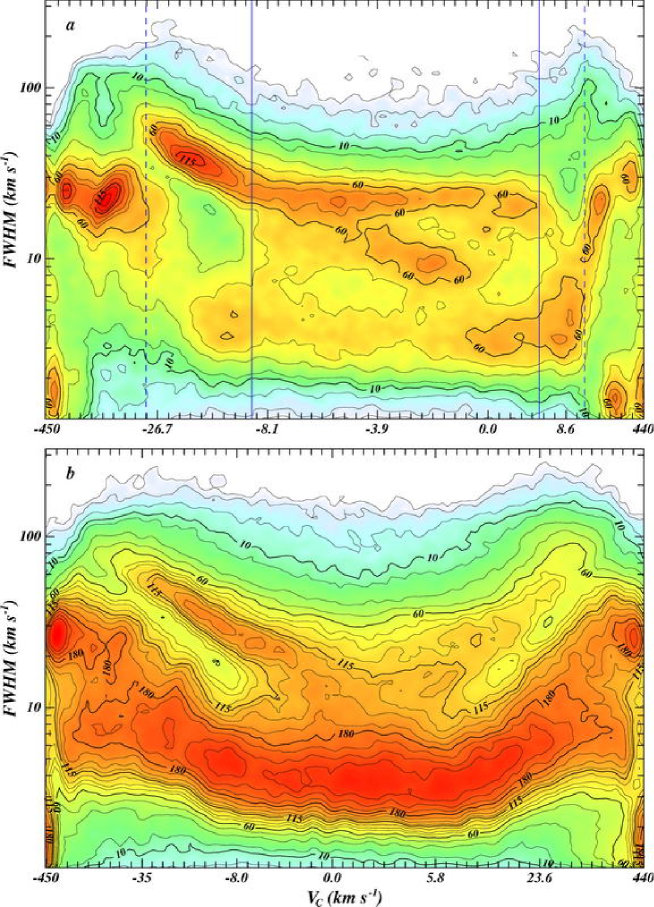
Figure 2: The distribution of Gaussian parameters in the central velocity – Gaussian width plane for two different latitude ranges: upper (a) panel for $|b|\geq 40\degr$ and the lower (b) one for $|b|<40\degr$. The contour lines on both panels are drawn at the levels of 1, 2, 5, 10, 15, 30, 45, 60, 75, 85, 100, 115, 125, 140, 160, 180, 200, 225, 250 and 300 Gaussians per counting bin. The ticks on the x-axis are drawn so that the number of Gaussians between every pair of neighbouring ticks is approximately the same. The precise values of the velocity corresponding to ticks of the upper panel are: $-450$, $-215$, $-120$, $-80$, $-60$, $-52$, $-47$, $-41$, $-36$, $-30.8$, $-26.7$, $-22.5$, $-19.1$, $-16.5$, $-14.4$, $-12.7$, $-11.3$, $-10.2$, $-9.4$, $-8.7$, $-8.1$, $-7.6$, $-7.1$, $-6.6$, $-6.2$, $-5.8$, $-5.4$, $-5.0$, $-4.6$, $-4.2$, $-3.9$, $-3.5$, $-3.16$, $-2.82$, $-2.47$, $-2.13$, $-1.77$, $-1.39$, $-0.95$, $-0.50$, 0.00, 0.59, 1.33, 2.21, 3.2, 4.6, 6.3, 8.6, 12.4, 21.6, 37, 70, 118, 207 and 440. Those for the lower panel are: $-450$, $-138$, $-107$, $-89$, $-74$, $-63$, $-54$, $-48$, $-41$, $-35$, $-30.3$, $-25.7$, $-22.0$, $-18.7$, $-15.8$, $-13.3$, $-11.3$, $-9.5$, $-8.0$, $-6.7$, $-5.5$, $-4.5$, $-3.6$, $-2.75$, $-1.97$, $-1.26$, $-0.59$, 0.00, 0.54, 1.08, 1.60, 2.10, 2.63, 3.2, 3.8, 4.4, 5.1, 5.8, 6.6, 7.5, 8.5, 9.7, 11.1, 12.6, 14.5, 16.9, 19.9, 23.6, 28.5, 35, 43, 52, 62, 73, 88, 107, 156 and 440. In panel a, the vertical solid lines enclose the velocity region $-9\leq V_{\mathrm{C}}\leq 4\leavevmode\nobreak\ \mathrm{km\,s}^{-1}$ of weak dependence of the line-widths on the central velocity of the components and the dashed lines correspond to the region $-31\leq V_{\mathrm{C}}\leq 18\leavevmode\nobreak\ \mathrm{km\,s}^{-1}$ discussed in the latter half of the paper.

From the relations discussed above, it follows that with the increasing mean velocity of the line also the line-width must increase. For our Gaussians this is illustrated in Fig. 2 separately for profiles at latitudes $|b|\geq 40\degr$ (upper panel) and $|b|<40\degr$ (lower panel). To construct both panels of this figure, we sorted in corresponding latitude intervals all Gaussians with central velocities in the decomposition range ($-460<V_{\mathrm{C}}<396\leavevmode\nobreak\ \mathrm{km\,s}^{-1}$ in the LDS2 and $-437<V_{\mathrm{C}}<451\leavevmode\nobreak\ \mathrm{km\,s}^{-1}$ in the IARS; for details see Papers I and II) in the ascending order of their central velocities and then grouped the sequence into 129 bins of an equal number of Gaussians, rejecting some Gaussians with the most extreme velocities. We binned the line-widths in equal steps of $\lg(\sigma_{V})$ of 0.025. The isolines in Fig. 2 give the numbers of Gaussians in each of such two-dimensional parameter interval. The latitude limit of $|b|=40\degr$ was chosen rather arbitrarily. For testing purposes, we constructed similar plots also by taking the limit at $|b|=30\degr$. In this case, the total number of Gaussians was increased in the upper panel and decreased in the lower panel, but the general structure of the distributions remained the same. Therefore, we may expect that the exact value of the limiting latitude is not very critical until it remains in some reasonable range.

The first thing we can see from Fig. 2 is that the typical line-widths of the density enhancements in the distribution of Gaussian parameters are not independent of the velocities of the Gaussians, but are larger for larger absolute values of the central velocities of the Gaussians. Moreover, this dependence seems to be stronger for lower latitudes than for higher ones, as expected from the relations discussed above. We can also see that at high velocities Figs. 2a ($|b|\geq 40\degr$) and 2b ($|b|<40\degr$) are rather similar (when we take into account the differences in the velocity scales of these plots). This is most likely caused by the fact that even near the galactic plane the amounts of the very high velocity gas remain modest, the corresponding Gaussians are relatively well separated from the bulk of the disk gas and their parameters are rather well defined.

At lower velocities, the differences are more remarkable. As discussed in detail in Paper II, there is much more gas near the galactic plane than at greater heights and therefore at low latitudes the effects of velocity crowding, blending and saturation become more severe and the profiles become more complex than at higher latitudes. As a result, the lower panel of Fig. 2 is dominated by the narrowest Gaussians and at larger widths we cannot distinguish other clear frequency enhancements. Most likely such a picture is caused by the fact that in this region the obtained Gaussians are only mathematically representing the profile and do not have any direct relation to the properties of the galactic H i. However, in the distribution of Gaussian widths at high galactic latitudes we can easily distinguish three frequency enhancements. Those with the smallest and largest widths correspond more or less to the enhancements visible also in the general distribution given in Fig. 1, but the concentration at intermediate widths is new, not unambiguously visible in the previous figure.

When the line-widths of the density enhancements in Figs. 2 are in general dependent of the central velocity of the corresponding Gaussians, they are nearly velocity independent in the region of $-9\la V_{\mathrm{C}}\la 4\leavevmode\nobreak\ \mathrm{km\,s}^{-1}$ (marked in Fig. 2a by two solid vertical lines). Therefore, in this velocity interval it would be also meaningful to estimate the mean line-widths of the three visible line-width groups of Gaussians. To obtain these estimates, we first found the distribution of the widths of all Gaussians with $|b|\geq 40\degr$, $-9\la V_{\mathrm{C}}\la 4\leavevmode\nobreak\ \mathrm{km\,s}^{-1}$ and modelled this distribution as a sum of three lognormal distributions defined by

$$f_{\mu,\sigma^{2}}(x)=\left\{\begin{array}[]{ll}0&(x\leq 0)\\ \frac{1}{\sqrt{2\pi}\sigma x}\mathrm{e}^{-\frac{(\ln(x)-\mu)^{2}}{2\sigma^{2}}}&(x>0)\,.\end{array}\right.$$ (2)

From many different density functions, more or less suitable for modelling the distribution of Gaussian widths, the values of which are defined to be positive, we have chosen to use the lognormal distribution, as its usage was technically rather convenient (if some parameter is distributed according to the lognormal law, the distribution of the logarithms of this parameter is described by a Gaussian). Mebold (Meb72 (1972)) has argued that his narrow and shallow components are more easily distinguishable when the line-width distribution is studied in logarithmic scale and in comparison with all initially tested distributions the lognormal one gave the best fits.

For the lognormal distribution, the mean value can be calculated as $\mathrm{M}(x)=\mathrm{e}^{\mu+\frac{\sigma^{2}}{2}}$, where $\mu$ and $\sigma$ may be considered as free parameters for fitting the model distribution to the observed one. In the case of Fig. 2a, we obtain for the means of three fitted distributions $\mathrm{FWHM}=3.89\pm 0.02$, $11.3\pm 0.1$ and $23.8\pm 0.2\leavevmode\nobreak\ \mathrm{km\,s}^{-1}$ (the error estimates here are the formal errors of the fit and do not account for errors in determination of the parameters of Gaussians or any possible systematic errors due to the applied data reduction methods).

The exact numerical values for the mean line-widths of the near zero velocity density enhancements in Fig. 2a also depend on the used velocity limits (solid vertical lines in Fig. 2a). These limits in their turn depend somewhat on the applied latitude limit for the separation of the panels in Fig. 2: the lower latitude limits tend to indicate more symmetrical velocity limits. However, for reasonable changes in latitude and velocity limits the changes in the width estimates are rather small. For example, when lowering the latitude limit to $|b|=30\degr$ and using the velocity limit $|V_{\mathrm{C}}|\la 8\leavevmode\nobreak\ \mathrm{km\,s}^{-1}$, we obtained the following mean width estimates: $\mathrm{FWHM}=3.78\pm 0.03$, $10.8\pm 0.2$ and $23.9\pm 0.5\leavevmode\nobreak\ \mathrm{km\,s}^{-1}$. The comparison of these numbers with the results given above also yields more realistic estimates of the actual reliability of the mean widths than the pure formal fitting errors.

4 The Gaussians from the simplest profiles

In the previous sections we used all the Gaussians obtained in the decomposition of all the profiles in the LAB database and tried to demonstrate how the distributions of their widths differ in different velocity or latitude regions. Finally, we concentrated our attention to the components with nearly zero velocity and to the relatively simple profiles at high galactic latitudes. Now we try to use the obtained information and limit ourselves to the simplest profiles and to the Gaussians describing only the low-velocity (relatively nearby) gas. Therefore, we must apply some selection criteria similar to those discussed in the previous section. First of all, as demonstrated by Fig. 2, we must exclude the complex profiles near the galactic plane. However, due to different complexity of the profiles in different longitude intervals the usage of a fixed latitude limit is probably not the best solution for this problem. Therefore, we decided to estimate the complexity of each profile individually.

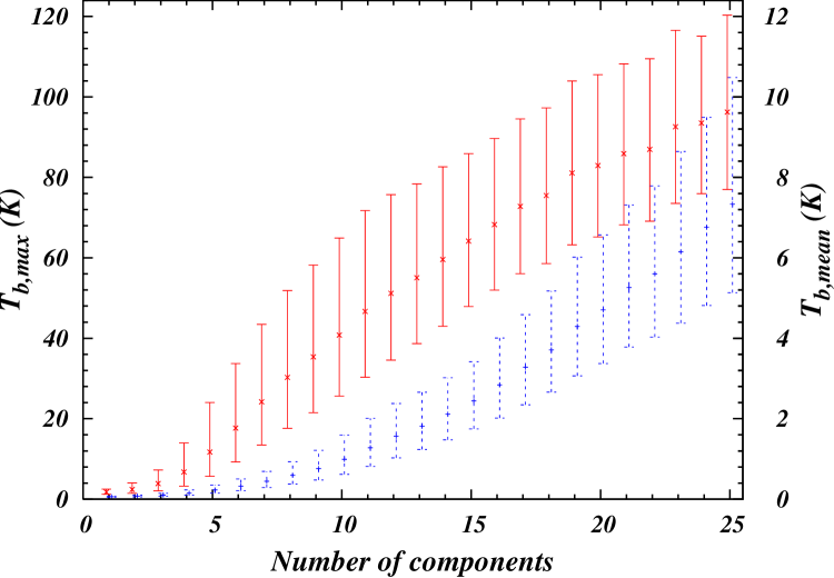
Figure 3: The relation between the number of Gaussians used for the decomposition of the profile, the peak brightness temperature (as estimated from the Gaussian decomposition) of the profile (red solid symbols, the vertical axis on the left) and the mean channel value in the region used for decomposition (blue dashed symbols, the vertical axis on the right). The errorbars represent the standard deviations around the mean of the corresponding distributions. The symbols are horizontally shifted to avoid overlap.

The complexity of the profile has two aspects. On the one hand, it is determined by the line formation process and to consider this, we must know the properties of the gas along the line of sight. In general, this information is not available and therefore we cannot directly distinguish the lines representing the superposition of the emission of many gas concentrations projected on each other from those formed by the emission of a relatively small number of gas clouds. However, on average, the brighter profiles are also more complex.

On the other hand, it is also important to know how well determined the parameters of the Gaussians obtained in the decomposition of every given profile are. In principle, this could be estimated. We have determined for every profile a set of Gaussian parameters, which corresponds to some minimal value of the residual rms of the deviations between the observed profile and its Gaussian representation. If we change the values of Gaussian parameters, the rms increases. The region within which the rms increases by no more than some predefined amount defines the confidence region around our solution. If we define the allowed increase of the rms so that the corresponding part of the parameter space contains some fixed percentage of the probability distribution of Gaussian parameters, the size and the shape of the confidence region give us the estimates for the errors of the obtained parameters. At the same time, this procedure requires huge amounts of computation, most likely not justified for the present study. However, on average, for profiles with a larger number of overlapping Gaussians the parameters of the latter are determined with lower confidence. Finally, as the number of Gaussians used for decomposition is rather well correlated with the emission content of the profile (Fig. 3), we choose as a primary indicator of the profile complexity the number of Gaussians needed for its decomposition.

However, in Paper II we demonstrated that some of the Gaussians are caused by different observational, reductional and decompositional problems and with high probability do not describe the properties of the galactic H i. As some profiles contain many spurious Gaussians, their inclusion in the analysis may considerably distort the profile complexity estimates. Therefore, before considering the complexity of the profiles, it is useful to exclude such Gaussians from consideration. We identify them by the criteria illustrated in Fig. 1 by thick solid lines. As described in Paper II, these criteria are analytically given by

$$\lg(\mathrm{FWHM})<0.057\lg(T_{\mathrm{b0}})^{2}-0.067\lg(T_{\mathrm{b0}})+0.094$$ (3)

(very narrow Gaussians are mostly due to stronger observational noise peaks and radio-interferences) and

$$\begin{array}[]{ll}\lg(T_{\mathrm{b0}})<&-0.370\lg(\mathrm{FWHM})^{3}+1.132\lg(\mathrm{FWHM})^{2}-\\ &1.567\lg(\mathrm{FWHM})+0.117\\ \end{array}$$ (4)

(most of the weakest components are caused by different uncertainties in the determination of the baselines for profiles). Here we are not interested in high-velocity clouds and therefore do not apply in the case of Eq. (4) any velocity limits used in Paper II, but we still reject all components with the central velocities outside the velocity range used for the decomposition. After rejection of these spurious components we classified the profiles on the basis of the total number of remaining Gaussians needed for the decomposition of any particular profile.

So far we have used in this section all the Gaussians irrespective of their central velocities. However, in the previous section we demonstrated that the mean line-widths of the components tend to increase with the increase of the absolute value of their central velocities. We also saw that this increase is slower for near zero velocities and becomes stronger at higher velocities. It is somewhat arbitrary to fix any numerical velocity limits for the regions with slow and faster line-width changes. In Fig. 2 these differences are also slightly exaggerated by the compression of the velocity scale at higher velocities. Nevertheless, when for the line-width group with widest Gaussians in Fig. 2a in the velocity interval of $|V_{\mathrm{C}}|\la 5\leavevmode\nobreak\ \mathrm{km\,s}^{-1}$ the mean line-width changes are not more than $0.25\leavevmode\nobreak\ \mathrm{km\,s}^{-1}$ per $1\leavevmode\nobreak\ \mathrm{km\,s}^{-1}$ of the central velocity change, for the velocity interval of $-30\la V_{\mathrm{C}}\la-10\leavevmode\nobreak\ \mathrm{km\,s}^{-1}$ this gradient increases at least to $1.5\leavevmode\nobreak\ \mathrm{km\,s}^{-1}$ per $1\leavevmode\nobreak\ \mathrm{km\,s}^{-1}$. Therefore, to restrict ourselves to the region of more or less constant mean line-widths, we accept for the following the velocity range appropriate for the higher latitude data and indicated in Fig. 2a by solid vertical lines. After such selection we separated in each class of profiles the Gaussians, central velocities of which fall into this range of $-9\leq V_{\mathrm{C}}\leq 4\leavevmode\nobreak\ \mathrm{km\,s}^{-1}$, and constructed for every class the distribution of the widths of these components.

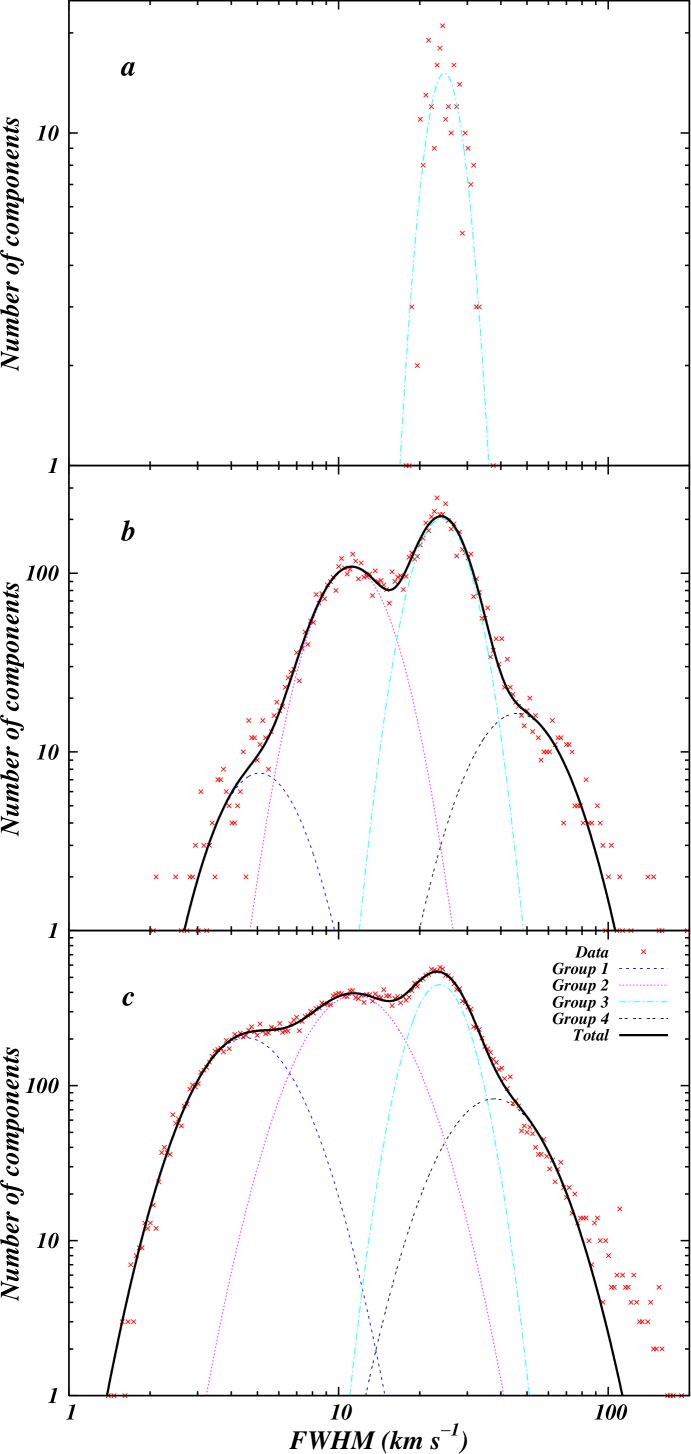
Figure 4: The distribution of the widths of Gaussians for the profiles decomposed to one (upper panel), two (middle panel) or three (lower panel) components.

It turned out that for profiles decomposed into one, two or three accepted Gaussians, the concentration of the widths around some distinct mean values was rather well defined without any additional selection criteria (Fig. 4). To estimate the mean widths characteristic of these different line-width groups, we once again modelled the obtained distributions as sums of lognormal distributions. As in Paper II we saw that the discrimination between the probably real and spurious Gaussians becomes more difficult at larger widths, we restricted the modelling process to the line-widths $\mathrm{FWHM}<100\leavevmode\nobreak\ \mathrm{km\,s}^{-1}$. Approximately above this width limit the selection criterion given by Eq. (4) becomes inoperative and at the greater widths no Gaussians are excluded by it. As a result, in these regions the proportion of the spurious components among the Gaussians, accepted for our analysis, may increase. This increase may be visible in the $\mathrm{FWHM}>100\leavevmode\nobreak\ \mathrm{km\,s}^{-1}$ region of Fig. 4c as a group of points above the fitted model line.

As can be seen from Fig. 4a, when the profile is successfully decomposed by only one low velocity Gaussian, such components belong exclusively to the line-width group 3, as defined by Fig. 4c. When the profile is decomposed by two Gaussians, the widths of corresponding components have already a much wider spread (Fig. 4b). Most of them still fall to group 3, but also to group 2, first discussed in connection with Fig. 2a, is well represented. Moreover, this is the case where group 2 is most clearly visible as a separate concentration of the line-widths. Beside these two dominating groups two weaker ones can be seen. On the left-hand side of the distribution, signs of group 1, which was the main group in Fig. 2b, become visible, but on the right-hand side the presence of a new group seems to be rather obvious.

In Fig. 4c the role of group 1 has considerably increased and it has become a well-established component of the distribution. The new fourth group still remains rather ill-defined. Moreover, as with more complex profiles the role of extremely wide Gaussians increases, the presence of group 4 becomes even somewhat more questionable than it may seem on the basis of Fig. 4b. Therefore, we add this new group to our list of the possible frequency enhancements in the distribution of the Gaussian widths, but we must remember that this group is established considerably less reliably than the other three.

On the basis of the profiles decomposed into one, two or three low velocity Gaussians, the estimates for the mean line-widths of the four groups of the components described above, are $4.9\pm 0.1$, $12.0\pm 0.3$, $24.4\pm 0.2$, and $43\pm 5\leavevmode\nobreak\ \mathrm{km\,s}^{-1}$. Unlike the previous estimates, here the errors are not given on the basis of the formal errors of the parameter fitting, but a procedure somewhat similar to bootstrap was used. We estimated the mean values and their formal errors separately for profiles with one, two or three Gaussians and also for any combination of such classes (the profiles with one and two or one and three Gaussians together and so on), calculated the weighted (on the basis of formal fitting errors) means of the results and accepted as an error the standard deviation of the obtained estimates from these means. We expect that such estimates include more realistically the uncertainties of the obtained values than the pure formal errors of the fit of the model to a fixed dataset.

For more complex profiles (four and more accepted Gaussians per profile) the components of the first group (the narrowest ones) become more and more dominating and this makes the recognition of the second group harder and harder (this is well demonstrated also by Fig. 2, where the second group is invisible in the lower panel, which represents the complex profiles near the galactic plane). The third group remains relatively well established, but the identification of the fourth group becomes increasingly complex and dependent on the accepted upper width limit, as in such profiles the frequency of extremely wide components increases. However, these changes are weaker for weaker profiles. At the same time, there is no clear-cut line between weak and strong profiles. Therefore, we decided to attempt to determine the width distributions of the Gaussians for different profile strength limits and we used in the following two different ways to define the profile strength. In the first case, we used as an indicator of the profile strength the peak brightness temperature of the profile (as estimated from the smooth Gaussian representation), but in the second case, we used the mean channel value (calculated from the original observed profile) over the velocity range used for decomposition.

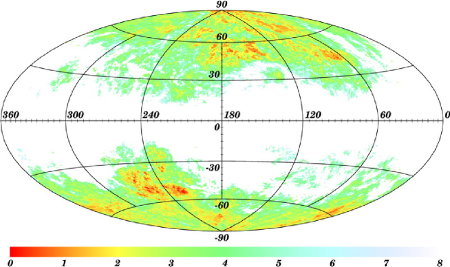
Figure 5: The sky positions of the 79 648 profiles used for the final line-width estimates. The positions of the simplest profiles are marked by the reddest dots. The colour scale represents in the first order the number of Gaussians per profile. Among the profiles with an equal number of Gaussians those with lower peak brightness temperature are plotted with redder colour.

For both profile strength definitions we repeated the estimates over a wide range of strength upper limits, but accepted for final results only the cases, where the means for all lognormal distributions were estimated with the formal errors below 50% (or 25% in a more restrictive case). In the case of the strength definition through the peak brightness temperature, the profile strength upper limit was increased in steps of $0.1\leavevmode\nobreak\ \mathrm{K}$ from the zero until there were no more acceptable results during the last 10 steps. Only for the profiles decomposed into three Gaussians even the inclusion of the strongest lines with the highest peaks extending up to $44.3\leavevmode\nobreak\ \mathrm{K}$ permitted determination of the parameters of different line-width groups. In all other cases no profiles with $T_{\mathrm{b,max}}>15.8\leavevmode\nobreak\ \mathrm{K}$ could be used and 89.7% of the profiles used for the final estimates had $T_{\mathrm{b,max}}\leq 12\leavevmode\nobreak\ \mathrm{K}$.

When using the peak brightness temperature as the profile strength indicator, the obtained mean line-widths were $4.3\pm 0.6$, $12.0\pm 0.5$, $24.1\pm 0.7$, and $42\pm 5\leavevmode\nobreak\ \mathrm{km\,s}^{-1}$ for the 50% maximal error limit and $4.6\pm 0.5$, $12.1\pm 0.4$, $24.1\pm 0.6$, and $41\pm 4\leavevmode\nobreak\ \mathrm{km\,s}^{-1}$ for 25%. Then the same procedure, but increasing the profile strength upper limit in steps of $0.001\leavevmode\nobreak\ \mathrm{K}$ was also repeated for the mean channel value as a profile strength indicator. In this case, the results were $3.9\pm 0.6$, $11.7\pm 0.4$, $24.1\pm 0.6$, and $43\pm 5\leavevmode\nobreak\ \mathrm{km\,s}^{-1}$ for the 50% limit and $4.3\pm 0.7$, $11.8\pm 0.4$, $24.1\pm 0.7$, and $42\pm 4\leavevmode\nobreak\ \mathrm{km\,s}^{-1}$ for 25%.

As we can see, the results are in general agreement within their error estimates, which consider the dispersion of the results for a particular selection process, but do not take into account the uncertainties related to the choice of the peak brightness or mean channel value as the profile strength indicator or the usage of the 25% or the 50% precision limit. As the results seem to depend more on the way of estimating the profile strength than on the limit of formal errors of the parameter determination, we accept as the final result the average over different profile strength estimates for the 50% error limit. After correcting the mean line-widths also for the width of the correlator channels in the LAB the corresponding values are: $3.9\pm 0.6$, $11.8\pm 0.5$, $24.1\pm 0.6$, and $42\pm 5\leavevmode\nobreak\ \mathrm{km\,s}^{-1}$. Altogether these estimates are based on the decomposition of 79 648 selected profiles. This set of profiles represents 42.0% of all observed sky positions in the LAB. The sky distribution of the corresponding profiles is given in Fig. 5.

As an additional check, we repeated the procedure described in this section also for the symmetrical velocity limit ($|V_{\mathrm{C}}|\leq 8\leavevmode\nobreak\ \mathrm{km\,s}^{-1}$ ) of the analysed profiles. As a profile strength indicator, we used the peak brightness and accepted the fits where the means for all lognormal distributions were estimated with the formal errors below 50%. In this case, we obtained the following values: $4.3\pm 0.5$, $12.0\pm 0.5$, $24.0\pm 0.7$, and $43\pm 5\leavevmode\nobreak\ \mathrm{km\,s}^{-1}$, the results still in good agreement with the earlier ones.

As we can see from Fig. 5, when selected on the basis of the number of Gaussians per profile and the strength of the emission line, the profiles used do not follow any well-defined latitude limit. Nevertheless, the mean values obtained for different line-width groups are still in good agreement with the estimates from the latitude limited samples obtained in Sec. 3. (we remind that the error estimates in these two cases are based on different considerations). This result, when combined also with Fig. 2, indicates that when there are clear differences in the overall line-width distribution of the most simple and most complex profiles, the transition from one to another is relatively smooth, without a well-defined boundary between them. Moreover, as differently selected samples give rather similar values for the mean line-widths of the groups, it seems that the width distributions of the profiles of different complexity differ from each other mainly by the degree of the presence of different line-width groups and not so much by the mean widths of these groups.

5 The comparison with earlier results

In the previous section we demonstrated that in the distribution of the widths of the Gaussians representing the simplest 21-cm line profiles of the galactic H i, we can distinguish at least three, but probably even four distinct groupings of the line-widths. Earlier, similar results have been reported by Verschuur and co-authors, who have published several papers (Ver89 (1989), Ver94 (1994), Ver99 (1999) hereafter VP, Ver02 (2002), Ver04 (2004) hereafter V4) where they argue that neutral hydrogen emission profiles produced by gas in the local interstellar medium are characterised by three, or probably four, line-width regimes where dominant and pervasive features have widths of the order $5.2\pm 0.4$ (VP regime 3), $12.8\pm 0.4$ (VP regime 2), $31.0\pm 0.5$ (VP regime 1b), and $50.1\pm 0.6\leavevmode\nobreak\ \mathrm{km\,s}^{-1}$ (VP regime 1a). They also note that these line-width regimes show a striking resemblance to a set of velocity regimes described by a plasma physical mechanism called the critical ionization phenomenon.

As we can see, our results are qualitatively identical. We both clearly distinguish three different groupings or regimes of the H i line-widths and admit that there may be also the fourth one with a larger mean line-width than the three main groups. However, we must recognize that there are considerable differences in the numerical values of the mean line-widths obtained by us and by Verschuur (as given in VP). On average, our results are about 17% smaller than those given in VP. The differences are the largest (approximately 22%) for groups 1 and 3 (VP regimes 3 and 1b) and the smallest (12%) for groups 2 and 4 (VP regimes 2 and 1a). At the same time, there are also considerable differences in our approaches to data analysis. Our studies are based on somewhat different initial data (the LAB instead of the published version of the LDS), we have used different Gaussian decomposition algorithms and selection criteria for choosing the components for final analysis. Our approaches to estimating the mean line-widths of the groups of the components are also different. Therefore, it is interesting to check how all these differences may have influenced the results obtained. As in most cases in his papers Verschuur has not given the results for his regime 1a, we follow the same practice in this section.

In Gaussian decomposition Verschuur and co-authors have clearly preferred the human assisted approach, as they assume that Gaussian decomposition “is not something that can be left to an idealized computer program” (VP). We have relied on the computer from the beginning (Paper I). The probability that the differences in decomposition algorithms may be the primary source of the discrepancies in the mean line-widths of our line-width groups and Verschuur’s regimes could be reduced if we could demonstrate that our programme gives for identical initial data practically the same results as obtained by Verschuur. This can be most easily done for the “random directions chosen from the Leiden/Dwingeloo data files” for which VP give in their Table 2 the list of sky positions from where the profiles of the sample have been chosen.

We analysed the Gaussians corresponding to these profiles of the LDS. In the width range of $0.5<\mathrm{FWHM}<60\leavevmode\nobreak\ \mathrm{km\,s}^{-1}$, used by VP (see Fig. 4b in VP), we found three concentrations of the line-widths around mean values of $\mathrm{FWHM}=5.4\pm 0.7$, $13.0\pm 0.5$ and $29.7\pm 6.8\leavevmode\nobreak\ \mathrm{km\,s}^{-1}$. In their Table 7, VP gave for the same sample the values equal to $5.2\pm 1.3$, $12.8\pm 1.2$ and $32.8\pm 1.8\leavevmode\nobreak\ \mathrm{km\,s}^{-1}$. As can be seen, for exactly the same initial data our results coincide within errors (here we use once again the formal errors of the fit).

The general selection criteria used by Verschuur are best described in the second chapter of V4. To test these criteria and to approximate the V4 results, we decomposed 206 671 profiles of the LDS (as published by Hartmann & Burton Har97 (1997)) into 1 644 665 Gaussians and applied the following selection criteria defined in accordance with our understanding of the criteria used in V4:

1. Profiles along the lines of constant Galactic longitude at $10\degr$ intervals, starting with $l=0\degr$ and every $1\degr$ in latitude were used.

2. The latitude range was from $|b|=80\degr$ (inc.) down toward the Galactic plane until:

   1. the latitudes $|b|<40\degr$ were reached, or

   2. the unsmoothed profile was found in which the brightness temperature in at least one channel in the velocity range of $-460<V_{\mathrm{C}}<396\leavevmode\nobreak\ \mathrm{km\,s}^{-1}$ was $10\leavevmode\nobreak\ \mathrm{K}$ or greater.

3. If the smooth profile, as reconstructed from the Gaussian decomposition, contained in the velocity interval of $-60\leq V_{\mathrm{C}}\leq 40\leavevmode\nobreak\ \mathrm{km\,s}^{-1}$ multiple peaks with separation less than $20\leavevmode\nobreak\ \mathrm{km\,s}^{-1}$ and the depth of the minimum between them less than 10% of the height of the lower peak, the Gaussians corresponding to this profile were not used in the analysis.

4. Any Gaussian with a peak brightness temperature of $<0.15\leavevmode\nobreak\ \mathrm{K}$ was removed from further consideration.

5. Only the components with the central velocity $V_{\mathrm{C}}$ in the range of $-31\leq V_{\mathrm{C}}\leq 18\leavevmode\nobreak\ \mathrm{km\,s}^{-1}$ were used for the study and all profiles requiring more than four such Gaussians were removed from the analysis.

Following V4, we analysed the results separately for positive and negative latitude data. For positive latitudes we obtained the mean values $\mathrm{FWHM}=4.5\pm 0.5$, $14.8\pm 1.7$, $30.4\pm 1.9\leavevmode\nobreak\ \mathrm{km\,s}^{-1}$ and for negative-latitudes we found $\mathrm{FWHM}=3.9\pm 0.5$, $11.5\pm 1.9$, $23.2\pm 0.4\leavevmode\nobreak\ \mathrm{km\,s}^{-1}$. We can see that on average these numbers are slightly larger than the corresponding results based on our selection criteria and the LAB data. Most likely this is due to the wider velocity range used by V4 (indicated in Fig. 2a by two dashed vertical lines). However, in the first order, these numbers must be compared with those given in Table 7 of V4: $\mathrm{FWHM}=5.8\pm 2.4$, $13.7\pm 2.3$, $35.1\pm 4.0\leavevmode\nobreak\ \mathrm{km\,s}^{-1}$ for positive and $\mathrm{FWHM}=5.2\pm 1.9$, $14.5\pm 2.4$, $33.9\pm 3.6\leavevmode\nobreak\ \mathrm{km\,s}^{-1}$ for negative latitude data, respectively (here our and V4 error estimates are most likely not directly comparable). With the exception of group 2, our values are still smaller than those by V4.

So far we have estimated the mean line-widths of the different line-width groups through the approximation of the distribution by the sum of lognormal functions. At the same time, the mean values given in Table 7 of V4 are calculated as averages over the predefined ranges of widths. If we apply the same approach and the same line-width ranges to our results described in this chapter, our mean line-widths are for positive-latitude data $\mathrm{FWHM}=5.7\pm 2.2$, $14.3\pm 2.8$, $34.4\pm 4.7\leavevmode\nobreak\ \mathrm{km\,s}^{-1}$ and for negative-latitude data $\mathrm{FWHM}=5.6\pm 2.2$, $14.2\pm 3.0$, $34.4\pm 4.9\leavevmode\nobreak\ \mathrm{km\,s}^{-1}$ (here the standard deviations of the line-widths around the means in predefined width intervals are given as error estimates as seems to have been done also by V4). These numbers are in good agreement with the V4 results as cited above. However, in this case it remains somewhat questionable how justified the averaging ranges used in V4 are. For example, why are in Table 7 of V4 the Gaussians with widths of $20<\mathrm{FWHM}<28\leavevmode\nobreak\ \mathrm{km\,s}^{-1}$ not included into any line-width regime?

6 Discussion

In V4 the obtained mean line-widths are used to estimate the kinetic temperatures of the gas. Verschuur found that the temperatures corresponding to the line-width regimes 1b and 3 are $24\,000\leavevmode\nobreak\ \mathrm{K}$ and $750\leavevmode\nobreak\ \mathrm{K}$, respectively. These temperatures were considered as physically unreal. On the basis of the coincidence of the obtained mean line-widths with the critical ionization velocities (CIV) for some atomic species ($6\leavevmode\nobreak\ \mathrm{km\,s}^{-1}$ for Na and Ca, $13.5\leavevmode\nobreak\ \mathrm{km\,s}^{-1}$ for C, N, and O, $34\leavevmode\nobreak\ \mathrm{km\,s}^{-1}$ for He and $51\leavevmode\nobreak\ \mathrm{km\,s}^{-1}$ for H, respectively) a model with collisionless gas, in which the origin of the profile broadening represents the influence of the critical ionization velocity effect, is presented. This interpretation has not found wide acceptance in astronomical community and our results make such explanation even more unlikely as the agreement between the selected CIVs and the mean line-widths seems to be poorer than stated by VP.

However, some decades ago, Clark (Cla65 (1965)) proposed a two-component model for interstellar H i where cold absorbing clouds are surrounded by hot, ubiquitous intercloud gas. Theoretical studies (e.g. Field et al. Fie69 (1969)) also demonstrated that the local H i could be considered as a two-phase medium, where much of the gas is either a warm neutral medium (WNM) with $T\sim 8000\leavevmode\nobreak\ \mathrm{K}$ or a cold neutral medium (CNM) with $T\sim 50\leavevmode\nobreak\ \mathrm{K}$ (Kulkarni & Heiles Kul87 (1987); Dickey & Lockman Dic90 (1990); Wolfire et al. Wol95 (1995); Ferrière Fer01 (2001)). At present this is one of the most widely accepted models for the local H i. Therefore, we try to check how our four line-width groups may be related to this model.

Mebold (Meb72 (1972)) has estimated that the emission line components, corresponding to the WNM, have a Gaussian dispersion of about $9.7\leavevmode\nobreak\ \mathrm{km\,s}^{-1}$ or $\mathrm{FWHM}\approx 23\leavevmode\nobreak\ \mathrm{km\,s}^{-1}$. This width is rather close to the mean width of our third line-width group and therefore we may expect that this line-width group may be related to the presence of the WNM in the ISM. With other line-width groups the situation seems to be somewhat more complicated.

Verschuur (Ver74 (1974)) and Schwarz & van Woerden (Sch74 (1974)) have demonstrated that the histogram of the CNM H i emission line widths peak around $\sigma_{V}=2.2\leavevmode\nobreak\ \mathrm{km\,s}^{-1}$, which corresponds to $\mathrm{FWHM}\approx 5.2\leavevmode\nobreak\ \mathrm{km\,s}^{-1}$ – a value somewhere between our first and second line-width groups and directly not comparable to any line-width group. However, here we must notice that their results have been obtained using all narrow emission line components presented in the observed profiles. At the same time, as discussed in the Introduction, for stronger emission components the saturation effects become important and this makes the line shape nongaussian and such lines seem to be broader than unsaturated profiles.

In our analysis we have used only relatively weak lines with nearly 90% of the used profiles having peak brightness less than $12\leavevmode\nobreak\ \mathrm{K}$. By combining the equation of radiative transfer with the approximate correlation between the H i spin temperature $T_{\mathrm{S}}$ and optical depth $\tau$ (e.g. Payne et al. Pay83 (1983)), we may estimate that for most of our profiles $\tau<0.1$, and therefore, we may use the approximation for optically thin gas $T_{\mathrm{b}}(\nu)=T_{\mathrm{S}}\tau(\nu)$. For $\tau\leq 0.1$ this approximation introduces up to 5% error in the peak brightness temperature of the emission profile, but practically does not change the line-width and consequently we must compare our line-widths not with those of much stronger emission lines cited above, but with the line-widths of the absorption lines of the CNM.

Crovisier (Cro81 (1981)) has reported that the distribution of the velocity dispersion inside the CNM clouds peaks around $1\leavevmode\nobreak\ \mathrm{km\,s}^{-1}$, but the mean value for the distribution is about $1.7\leavevmode\nobreak\ \mathrm{km\,s}^{-1}$. The latter corresponds to $\mathrm{FWHM}\approx 4.0\leavevmode\nobreak\ \mathrm{km\,s}^{-1}$, which coincides within errors with the mean line-width of our first line-width group. This makes it rather plausible that the existence of both line-width groups 1 and 3 is a reflection of the presence of two thermal phases of neutral gas in the local interstellar medium.

Theoretical CNM and WNM temperatures are derived by calculating the equilibrium temperature as a function of thermal pressure. As pointed out above, there exist two stable ranges of equilibrium, separated by a region of unstable temperatures. If we interpret the line-width of group 2, $11.8\leavevmode\nobreak\ \mathrm{km\,s}^{-1}$, as thermal, the corresponding kinetic temperature would be about $3000\leavevmode\nobreak\ \mathrm{K}$, which lies just in the region of unstable temperatures. At the same time, the presence of some gas with such temperatures seems to have been a long-standing problem. Cox (Cox05 (2005)) has recently given a review of the three-phase model of the interstellar medium, but there the additional third phase (warm H ia) has a temperature of $5000\leavevmode\nobreak\ \mathrm{K}$. Heiles (Hei01 (2001)) and Heiles & Troland (Hei03 (2003)) have reported that at least 48% of the WNM lies in the thermally unstable region of $500-5000\leavevmode\nobreak\ \mathrm{K}$. Similar results were obtained by Mebold et al. (Meb82 (1982)). On the basis of the results by Dickey et al. (Dic77 (1977, 1978, 1979)), Crovisier (Cro81 (1981)) discussed the presence of cold clouds, lukewarm clouds and not strongly absorbing material. Therefore, with some probability our line-width group 2 may also represent thermally unstable neutral gas and our (also Verschuur’s) results (Fig. 2a and especially Fig. 4b) demonstrate that this is not just a tail of the CNM or the WNM temperature distribution, but a component in its own rights.

Besides first three rather obvious line-width groups there is also the line-width group 4 with the mean line-width around $42\leavevmode\nobreak\ \mathrm{km\,s}^{-1}$. As mentioned above, the real existence of this group is much more questionable, as it may be seriously affected by baseline and stray radiation corrections in the survey (see Paper 2). Therefore, we make only some brief remarks about this group. Kalberla et al. (Kal98 (1998)) have argued in favour of the existence of some neutral gas in the galactic halo. The mean velocity dispersion of this gas is $\sigma=60\pm 3\leavevmode\nobreak\ \mathrm{km\,s}^{-1}$ at the north galactic pole and it increases at lower latitudes. The corresponding H i line-widths must be more than 3 times higher than the mean for our line-width group 4. Line-widths (with $\sigma=21\pm 4\leavevmode\nobreak\ \mathrm{km\,s}^{-1}$) much more similar to our group 4 are reported from the measurements of absorption lines by Dwarakanath (Dwa04 (2004)) and Mohan et al. (2004a ; 2004b ).

It is also interesting to estimate the mass fractions of the H i gas, corresponding to the described four line-width groups. However, in our case these estimates are made rather questionable by at least two factors. First of all, the line components with highest peak brightness temperatures belong to the line-width group 1 and in the following groups the components are on average progressively weaker. As for our estimates we have selected only the simplest and the weakest profiles, we have biased the mass fraction estimates in favour of the groups with wider and weaker line components. Therefore, for the estimates of mass fractions, it is more natural to return to our latitude limited samples (similar to Fig. 2a), but even in this case the stronger lines near the galactic plane become optically thicker, which causes the underestimation of corresponding masses.

The second problem is that when the mean line-widths of our line-width groups are well determined by log-normal fits, the standard deviations of the corresponding distributions are rather poorly constrained due to correlations between these parameters for different line-width groups. To obtain the fits for different latitude limits $|b|\geq b_{\mathrm{lim}}$, we had therefore to restrict the variability of these parameters and this probably introduces some systematic errors into the mass fraction estimates, specially for lower values of $b_{\mathrm{lim}}$.

Nevertheless, we found that for $|b|\geq 40\degr$ the velocity interval of $-9<V_{\mathrm{C}}<4\leavevmode\nobreak\ \mathrm{km\,s}^{-1}$ contains more than 51% of all H i. As the line-width groups found in this velocity interval seem to continue even beyond the accepted velocity limits (with the exception of group 2, which is visible only in the vicinity of $V_{\mathrm{C}}=0\leavevmode\nobreak\ \mathrm{km\,s}^{-1}$, they just become smoothly wider at higher velocities), we may conclude that the described line-width concentrations are characteristic of most of the high-latitude H i.

The distribution of the H i between the obtained line-width groups depends on the latitude limit used. Only the relative content of group 4 is about 4% for all samples $|b|\geq b_{\mathrm{lim}}$ with different values of $b_{\mathrm{lim}}$. For $15\degr\ga b_{\mathrm{lim}}\ga 55\degr$ the relative fractions of other groups change rather slowly and smoothly. The share of groups 1 and 2 decreases from about 18% and 45% for $|b|\geq 15\degr$ to about 11% and 39% at $|b|\geq 55\degr$, respectively. However, we must stress once more that the estimates for these groups are strongly correlated and especially for lower galactic latitudes the actual fraction of group 1 may be higher and that of group 2 lower than stated here. The content of group 3 increases for the same latitude range from about 34% to 46%. For larger values of $b_{\mathrm{lim}}$ the relative fraction of group 1 remains at about 11%, but the share of group 2 quickly increases to about 47% at $b_{\mathrm{lim}}=75\degr$ and that of group 3 drops to about 37%. Therefore, for most of the relatively high-latitude gas we, like Heiles (Hei01 (2001)), may conclude that about half of the WNM is represented by line-width group 2 which temperatures lie in the thermally unstable regime. For $b_{\mathrm{lim}}<15\degr$ our analysis is most likely not applicable at all and for $b_{\mathrm{lim}}\geq 75\degr$ the results become uncertain due to the small number of profiles.

7 Conclusions

We have demonstrated that for simple (Sec. 4.) and high-latitude (Sec. 3.) profiles the line-widths of the H i emission profiles exhibit concentration to certain preferred line-width groups. With this we confirm and extend the earlier similar results obtained by Verschuur and co-authors (Ver89 (1989), Ver94 (1994), Ver99 (1999), Ver04 (2004)). We define the limits of the usable velocities ($-9\leq V_{\mathrm{C}}\leq 4\leavevmode\nobreak\ \mathrm{km\,s}^{-1}$) on the basis of the extent of the region, where the dependence of the line-widths on the component velocities is the weakest. We have not fixed any exact criteria for the simplicity of the profiles, but have tried instead many different combinations of the limits on the number of the Gaussians in the decomposition and on the profile strength as defined by their peak brightness or mean channel value. For the final results we have accepted only these combinations of the limits, which allow the determination of the mean line-widths of all width groups with the formal fitting errors less than 50%. This condition was fulfilled for all profiles, decomposed into one, two or three components. For such profiles we demonstrated that it is possible to distinguish three or four groups of preferred line-widths. The existence of groups 2 and 3 is very clearly visible, when using only the profiles decomposable by one or two Gaussians (Figs. 4a and 4b). Group 1 can be better distinguished in profiles decomposed by three components (Fig. 4c). The reality of group 4 remains more questionable. A similar separation was possible also for weaker profiles decomposed into four, or in some cases even into up to 7 Gaussians. The mean line-widths of the groups found are $3.9\pm 0.6$, $11.8\pm 0.5$, $24.1\pm 0.6$, and $42\pm 5\leavevmode\nobreak\ \mathrm{km\,s}^{-1}$.

The mean line-widths obtained by us are somewhat smaller than those proposed earlier by Verschuur. The disagreement may be caused partly by different algorithms used to measure the mean line-widths of our groups and VP regimes. Another important point appears to be the usage by V4 of Gaussians from a considerably wider velocity range than it is acceptable to us. Due to the smaller mean line-widths of our line-width groups, also the interpretation of the existence of the corresponding groups through the collisionless gas and critical ionization velocities, as proposed by Verschuur, seems rather questionable to us. More likely groups 1 and 3 represent CNM and WNM components of the ISM. The existence of group 2, which may represent up to 40% of all H i, in the thermally unstable regime, is in conflict with usual two component equilibrium models of the ISM, but from our data (Figs. 2a and 4b) the existence of such a group seems to be well established. The reality and the origin of the broad lines with the widths of about $42\leavevmode\nobreak\ \mathrm{km\,s}^{-1}$ is more obscure. These, however, contain only about 4% of the total observed column densities.

- (1) Bajaja, E., Arnal, E. M., Larrarte, J. J., et al. 2005, A&A, 440, 767
- (2) Clark, B. G. 1965, ApJ, 142, 1398
- (3) Cox, D. P. 2005, ARA&A, 43, 337
- (4) Crovisier, J. 1981, A&A, 94, 162
- (5) Dickey, J. M., & Lockman, F. J. 1990, ARA&A, 28, 215
- (6) Dickey, J. M., Salpeter, E. E., & Terzian, Y. 1977, ApJ, 211, L77
- (7) Dickey, J. M., Salpeter, E. E., & Terzian, Y. 1978, ApJS, 36, 77
- (8) Dickey, J. M., Salpeter, E. E., & Terzian, Y. 1979, ApJ, 228, 465
- (9) Dwarakanath, K. S. 2004, BASI, 32, 215
- (10) Ferrière, K. M. 2001, Rev. Mod. Phys., 73,1031
- (11) Field, G. B., Goldsmith, D. W., & Habing, H. J. 1969, ApJ, 155, L149
- (12) Hartmann, L. 1994, The Leiden/Dwingeloo Survey of Galactic Neutral Hydrogen, Ph. D.-Thesis, Leiden Univ.
- (13) Hartmann, L., & Burton, W. B. 1997, Atlas of Galactic Neutral Hydrogen, Cambridge Univ. Press, 10+236 pp
- (14) Haud, U. 2000, A&A, 364, 83 (Paper I)
- (15) Haud, U., & Kalberla, P. M. W. 2006, Balt. Astron., 15, 413 (Paper II)
- (16) Heiles, C. 2001, ApJ, 551, L105
- (17) Heiles, C., & Troland, T. H. 2003, ApJ, 586, 1067
- (18) Kalberla, P. M. W., Westphalen, G., Mebold, U., Hartmann, D., & Burton, W. B. 1998, A&A, 332, L61
- (19) Kalberla, P. M. W., Burton, W. B., & Hartmann, D., et al. 2005, A&A, 440, 775
- (20) Kulkarni, S. R., & Heiles, C. 1987, in Interstellar Processes, ed. D. Hollenbach, & H. A. Thronson, Jr. (Dordrecht: Reidel), 87
- (21) Mebold, U. 1972, A&A, 19, 13
- (22) Mebold, U., Winnberg, A., Kalberla, P. M. W., & Goss, W. M. 1982, A&A, 115, 223
- (23) Mohan, R., Dwarakanath, K. S., & Srinivasan, G. 2004, JApA, 25, 143
- (24) Mohan, R., Dwarakanath, K. S., & Srinivasan, G. 2004, JApA, 25, 185
- (25) Payne, H. E., Salpeter, E. E., & Terzian, Y. 1983, ApJ, 272, 540
- (26) Schwarz, U. J., & van Woerden, H. 1974, in Galactic Radio Astronomy, ed. F. J. Kerr, & S. C. Simonson III (Dordrecht: Reidel), 45
- (27) Verschuur, G. L. 1974, ApJS, 27, 65
- (28) Verschuur, G. L., & Schmelz, J. T. 1989, AJ, 98, 267
- (29) Verschuur, G. L., & Magnani, L. 1994, AJ, 107, 287
- (30) Verschuur, G. L., & Peratt, A. L. 1999, AJ, 118, 1252 (VP)
- (31) Verschuur, G. L. 2002, AAS Meeting 200, #73.03
- (32) Verschuur, G. L. 2004, AJ, 127, 394 (V4)
- (33) Westphalen, G. 1997, Ph.D.-Thesis, Bonn Univ.
- (34) Wolfire, M. G., Hollenbach, D., McKee, C. F., Tielens, A. G. G. M., & Bakes, E. L. O. 1995, ApJ, 443, 152