Tracing the long bar with red-clump giants

Abstract

Context. Over the last decade a series of results have lent support to the hypothesis of the existence of a long thin bar in the Milky Way with a half-length of 4.5 kpc and a position angle of around 45^∘. This is apparently a very different structure from the triaxial bulge of the Galaxy.

Aims. In this paper, we analyse the stellar distribution in the inner 4 kpc of the Galaxy to see if there is clear evidence for two triaxial or barlike structures, or whether there is only one.

Methods. By using the red-clump population as a tracer of the structure of the inner Galaxy we determine the apparent morphology of the inner Galaxy. Star counts from 2MASS are used to provide additional support for this analysis.

Results. We show that there are two very different large-scale triaxial structures coexisting in the inner Galaxy: a long thin stellar bar constrained to the Galactic plane ($|b|<2^{\circ}$) with a position angle of 43$\aas@@fstack{\circ}$0$\pm$1$\aas@@fstack{\circ}$8, and a distinct triaxial bulge that extends to at least $|b|\leq 7.5^{\circ}$ with a position angle of 12$\aas@@fstack{\circ}$6$\pm$3$\aas@@fstack{\circ}$2. The scale height of the bar source distribution is around 100 pc, whereas for the bulge the value of this parameter is five times larger.

1 Introduction

There is now a substantial consensus for there being a stellar bar in the inner Galaxy. This was first suggested by de Vaucouleurs (1964) to explain the nonaxisymmetry in radio maps. The first evidence for a barlike distribution in the stars was derived from the asymmetries in the infrared (IR) surface brightness maps (e.g. Blitz & Spergel 1991; Dwek et al. 1995) and in source counts (Weinberg 1992; Hammersley et al. 1994; Stanek et al. 1994), which both show systematically more stars at positive galactic longitudes $l<30$ close to the Galactic plane (GP). The exact morphology of the inner Galaxy, however, is still controversial. While some authors refer to the bar as a fatter structure, around 2.5 kpc in length with a position angle of 15–30 degrees with respect to the Sun–Galactic Centre direction (Dwek et al. 1995; Nikolaev & Weinberg 1997; Stanek et al. 1997; Binney et al. 1997; Freudenreich 1998; López-Corredoira et al. 1999; Bissantz & Gerhard 2002; Babusiaux & Gilmore 2005), other researchers suggest that there is a long bar with a half length of 4 kpc and a position angle of around 45 degrees. It is noteworthy that those authors supporting the $23^{\circ}$ bar all examine the region at $|l|<12^{\circ}$, whereas those supporting the long bar with the larger angle are trying to explain counts for $10^{\circ}<l<30^{\circ}$ and $-10^{\circ}>l>-30^{\circ}$.

Hammersley et al. (2000) showed that there is a major over-density of K2-3III (red-clump) stars on the GP at $l=27^{\circ}$ at a distance of about 6 kpc from the Sun. This over-density could also be detected at smaller galactic longitudes, but more reddened and at an increased distance from the observer. These stars could not be seen a few degrees above or below the GP at the same galactic longitudes, nor at greater longitudes. This, when combined with the findings of Hammersley et al. (1994), was interpreted as strong evidence for the existence of a long in-plane bar with a half length $\sim$4 kpc and position angle of 43^∘, clearly distinguishable from the triaxial bulge, but running into it near $l$=12^∘. This over-density of stars was also analysed by comparing near-infrared (NIR) counts with predictions of the Besançon Galactic model (Robin et al. 2003) with similar conclusions (Picaud et al. 2003). This result has been further supported by observations in the mid-infrared with GLIMPSE data (Benjamin et al. 2005) who did a similar analysis to that of Hammersley et al. (2000) but at a wavelength range in which the effects due to extinction are even lower than in the NIR, hence reducing the uncertainty in the results.

There is also a noticeable difference in the luminosity function found in the two regions. The majority of the work on the short, fat bar (subtending an angle of $\sim$23^∘ with the Sun–Galactic Centre line), has been restricted to within a few degrees of the plane in regions that are routinely used by other authors to study the bulge, and what is seen is an older population. The on-plane region between $l=20^{\circ}$ and 27^∘, however, has been shown to contain a large number of extremely luminous young stars (Hammersley et al. 1994; Gazón et al. 1997; López-Corredoira et al. 1997), and a characteristic feature of long bars is a major star formation region where they interact with the disc.

These results suggest that the structure in the inner Galaxy ($|l|<12^{\circ}$) could be interpreted as a triaxial bulge rather than a bar, and certainly not a long straight bar. This triaxial bulge has axial ratios of 1:0.5:0.4 (López-Corredoira et al. 2005). Furthermore López-Corredoira et al. (1999) showed that a triaxial bulge + disc model cannot reproduce the observed counts in the Galactic plane for $10^{\circ}<l<30^{\circ}$. This is also suggested by NIR photometry of red-clump stars (Nishiyama et al. 2005). It should be noted that the possibility of there being even smaller non-axisymmetric structures (e.g. a secondary bar) in The Milky Way cannot be discounted (Unavane & Gilmore 1998; Alard 2001; Nishiyama et al. 2005); thus, more observations are needed for a decisive conclusion to be reached.

Many galaxies have triaxial bulges contained within a primary stellar bar, and even a third, smaller-scale bar inside the bulge (Fiedli et al.  1996). More than half of all disc galaxies have some kind of bar component (Buta, Crocker & Elmegreen 1996) and as many as a third have a strong primary bar (Freeman 1996). Recent NIR observations by Beaton et al. (2005) and $N$-body simulations by Athanassoula & Beaton (2006) provide strong evidence in favour of the existence in our close neighbour M31 of a boxy bulge contained within a primary bar of semilength of $\sim$4 kpc. Such a high degree of morphological similarity between two neighbouring galaxies is striking (even though the angular separation between the major axes of the primary bar and triaxial bulge is different for the two galaxies).

Bars are generally constrained to the plane whereas bulges are shorter and more extended vertically. Therefore, using data covering a wide range of longitudes and latitudes is the only way to distinguish between the two possible morphologies for the inner Milky Way: a short inner bar or a triaxial bulge + long bar. In this paper we have used NIR data from the TCS-CAIN survey to analyse the spatial distribution of red-clump sources in the inner Galaxy. This population of stars has been widely used as a standard candle in deriving distances to the inner Galaxy (Hammersley et al 2000; Stanek et al. 1994; López-Corredoira et al. 2004; Babusiaux & Gilmore 2005; Nishiyama et al. 2005, 2006b). By observing how these stars are distributed along different lines of sight towards the inner Galaxy we are able to explore the 3D morphology of our Galaxy.

2 TCS-CAIN catalogue

TCS-CAIN catalogue is a NIR survey of the Milky Way that has recently been completed at the Instituto de Astrofísica de Canarias. This survey consists of more than 500 fields distributed along or near the Galactic plane ($|b|\leq 10^{\circ}$) observed in $J$, $H$ and $K_{\rm s}$ filters with a photometric accuracy of $\sim$0.1 mag in the three bands and a positional accuracy of $\sim$0.2^′′, based on the 2MASS catalogue as astrometric reference. Each field covers approximately 0.07 deg² on the sky, centred on the stated galactic coordinates for that field. The nominal limiting magnitudes of the survey (determined using growth curves of the differential star counts) are 17, 16.5 and 15.2 in $J$, $H$ and $K_{\rm s}$ respectively; hence, TCS-CAIN is at least one magnitude deeper than 2MASS, and even more in the inner Galaxy, where confusion is important. A complete description of the catalogue and data reduction, and details of its contents can be found in Cabrera-Lavers et al. (2006).

In this paper we have used all the available near plane fields in the inner Galaxy ($|l|<30^{\circ}$, $|b|$$\leq$7.5^∘), which gives a total number of 205 usable fields, covering an area of approximately 14.2 deg² of the sky (nearly 35% of the whole catalogue area).

3 Red-clump stars as a distance indicator

Red-clump giants have long been proposed as standard candles. They have a very narrow luminosity function and constitute a compact and well-defined clump in an HR diagram, particularly in the infrared. Furthermore, as they are relatively luminous, they can be identified even to large distances from the Sun. López-Corredoira et al. (2002) developed a method to obtain the star density and interstellar extinction along a line of sight by extracting the red-clump population from the NIR colour–magnitude diagrams (CMDs). This method has proved very powerful for analysing the structure of the thin (López-Corredoira et al. 2002, 2004) and thick (Cabrera-Lavers et al. 2005) discs of the Milky Way, as well as in the study of the distribution of interstellar extinction (Drimmel et al. 2003; Picaud et al. 2003; Duran & van Kerkwijk 2006).

The absolute magnitude ($M_{K}$) and intrinsic colour, $(J-K_{\rm s})_{0}$, of the red-clump giants are well established (Alves 2000; Grocholski & Sarajedini 2002; Salaris & Girardi 2002; Pietrzyński et al. 2003). Here, we consider an absolute magnitude for the red clump population of $-1.62\pm 0.03$ mag and and an intrinsic colour of $(J-K_{\rm s})_{0}$ = 0.7 mag. These values are consistent with the results derived by Alves (2000) from the Hipparcos red-clump and also with the results obtained by Grocholski & Sarajedini (2002) for open clusters. The intrinsic colour of the red-clump stars predicted by the Padova isochrones in the 2MASS system (Bonatto et al. 2004) for a 10 Gyr population of solar metallicity is $(J-K)_{0}$ = 0.68 mag. As 2MASS photometry is nearly equivalent to the TCS-CAIN photometric system (Cabrera-Lavers et al. 2006) the value of 0.7 mag is sufficiently close to represent the red-clump population.

The absolute magnitude of the red-clump has a small dependence on metallicity (Salaris & Girardi 2002). There is no large metallicity gradient in the Galactic disc (Ibata & Gilmore 1995a,b; Sarajedini et al. 1995); however, there is a slight difference between the solar neighborhood metallicity and those of the bulge giants, which peaks at [Fe/H] = $-0.25$ dex (Ramírez et al. 2000; Schultheis et al. 2003; Molla et al. 2000). According to Salaris & Girardi (2002), a small correction of 0.03 mag should be applied to the absolute magnitude of the red-clump stars for these ranges of metallicity. However, this is well within the uncertainty considered for the absolute magnitude used here. The red-clump absolute magnitude in $J$ is more sensitive to metallicity and age than the $K$ filter, hence the intrinsic colour $(J-K)_{0}$ also depends on both the metallicity and age (Salaris & Girardi 2002; Grocholski & Sarajedini 2002; Pietrzyński et al. 2003). The theoretical isochrones of Salaris & Girardi (2002) and Bonatto et al. (2004) suggest that the de-reddened colour for the range of metallicities expected for a bulge population is $(J-K)_{0}=0.63\pm 0.02$. Hence the metallicity dependences lead to a systematic uncertainty of 0.03 mag in the absolute magnitude of the red-clump stars and 0.05 mag in the intrinsic colour, $(J-K)_{0}$.

A recent study using NIR spectra of the inner Galaxy giants between $20^{\circ}<l<30^{\circ}$ has shown that these stars have a well defined metallicity (typically [Fe/H] between 0 and $-0.2$ dex) with a very small dispersion (Cabrera-Lavers et al., in preparation). By using the population of infrared carbon stars from the 2MASS survey, Cole & Weinberg (2002) conclude that the bar formed more recently than 3 Gyr ago and must be younger than 6 Gyr. For this age and metallicity, the corrections given by Salaris & Girardi (2002) are even lower than for the older bulge. Hence, we have assumed that uncertainties in absolute magnitude and intrinsic colour for this population of red-clump stars are of the same order as in the case of the bulge stars.

In this paper the TCS-CAIN survey data is analysed using the method developed by Stanek et al. (1997) for their data obtained by the Optical Gravitational Lensing Experiment (OGLE; Udalski et al. 1993,1994). This method has also recently been used by Nishiyama et al. (2005, 2006b) and Babusiaux & Gilmore (2005) to analyse the red-clump population of the inner Galaxy.

To avoid extinction effects a reddening-independent magnitude ($K_{e}$) is used:

$$K_{e}=K_{s}-\frac{A_{K_{\rm s}}}{A_{J}-A_{K_{\rm s}}}(J-K_{\rm s}),$$ (1)

adopting $A_{K_{\rm s}}/E_{J-K_{\rm s}}=0.68$ (Rieke & Lebofski 1985), a value which agrees with that used in Babusiaux & Gilmore (2005) and also with that obtained by Indebetouw et al. (2005) by combining data from the Spitzer Space Telescope and 2MASS.

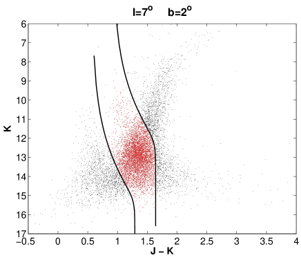
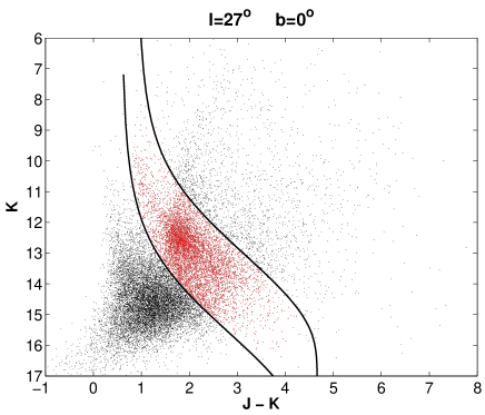
Figure 1: Two examples of the use of the theoretical traces for the giant population by means of the SKY model. Stars isolated between both traces (corresponding to the K0 and the M0 populations) are assumed to be red-clump stars and are extracted to analyse their spatial distribution.

With the reddening-independent magnitudes, any compact structural feature in the CMD would appear as a “clump” of stars, as they will be located at approximately the same distance from the Sun and hence they would have the same apparent $K$-magnitude. As the red-clump stars are the dominant giant population (Cohen et al. 2000; Hammersley et al. 2000), we can derive the distance to the feature by a non-linear least-squares fit of the sum of a Gaussian function and a second-order polynomial (eq. 2) to the histogram of red giant stars (Stanek et al. 1994; Stanek & Garnavich 1998; Babusiaux & Gilmore 2005):

$$N(m)=a+bm+cm^{2}+\frac{N_{\rm RC}}{\sigma_{\rm RC}\sqrt{2\pi}}\exp\left[-\frac{(m_{\rm RC}-m)^{2}}{2\sigma_{\rm RC}^{2}}\right].$$ (2)

The Gaussian term corresponds to a fit of the red-clump population of the bulge/bar, while the second-order polynomial reflects the contribution of the background stars. The combined effect of distance plus extinction produces an increase in the mixture between faint dwarfs and giants. In order to subtract the contribution of foreground dwarf stars we have used the SKY extinction model (Wainscoat et al. 1992) to derive the theoretical traces in the diagrams for the giant population in each field. With these theoretical traces we can isolate the population of red-clump stars in each CMD; thus, the fit is made only after removing the contribution of dwarf stars in the reddening-corrected counts (Fig. 1).

To transform the derived extinction-corrected magnitudes into distances from the Sun we use:

$$\mu_{K}=K_{e}+\frac{A_{K_{\rm s}}}{A_{J}-A_{K_{\rm s}}}(J-K_{s})_{0}-M_{K}.$$ (3)

To estimate an upper limit to the reddening-independent magnitude that can be analysed reliably we have followed the same procedure described in Babussiaux & Gilmore (2005). First, an estimate of the completeness limits in $J$ and $K$ ($J_{\rm C},K_{\rm C}$) are derived by determining when the number counts as function of magnitude stops increasing. The relative completeness of $K_{e}$ is then derived by combining these estimates with the mean colour of the giants in the field $(J-K)_{\rm M}$, and adding a 0.5 mag safety margin to take into account the spread in the mean colour:

$$max(K_{e})=min(J_{\rm C}-(J-K)_{M},K_{\rm C})-\left(\frac{A_{K}}{E_{J-K}}(J-K)_{\rm M}\right)+0.5.$$ (4)

Figure 2 shows all of the analysed fields used in this work. There are three different kind of fields:

• Those (labelled “discarded” fields) in which the completeness made it impossible to fit the red-clump distribution accurately.

• Those (labelled “rejected” fields) in which no successful fit was possible, as no clear structural component was present. In these cases, the counts increase continuously with the distance modulus until reaching the completeness limit for the field. These in-plane fields are purely disc fields and are located too far above or below the galactic plane for either the bulge or the bar components to be observed, so that no “hump” in the red-clump counts is expected (Fig. 3).

• Those marked as “used” in Fig. 2 where it was possible to derive a distance to the red-clump population. After discarding all those fields which were not useful, we obtained results in 49 of the total sample of 205 fields.

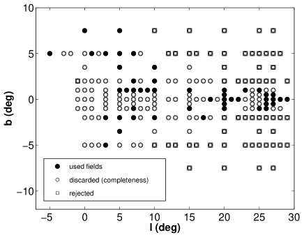
Figure 2: Summary of the 205 TCS-CAIN fields analysed in this work.

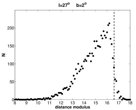
Figure 3: Example of a field where no peak in the counts of the red-clump distribution is observed, as we are observing a field where only the disc component is present, hence the star counts increase up to the completeness limit of the field (shown as a vertical dashed line).

3.1 Distances derived with $H/J-H$ data

Some fields were observed only in the $J$ and $H$ bands, since far from the Galactic plane the counts in the $K$ and $H$ bands are nearly equivalent due to the low extinction. For this reason some of the fields in this work use $H$-band extinction-corrected magnitudes ($H_{e}$):

$$H_{e}=H-\frac{A_{H}}{A_{J}-A_{H}}(J-H),$$ (5)

$$\mu_{H}=H_{e}+\frac{A_{H}}{A_{J}-A_{H}}(J-H)_{0}-M_{H},$$ (6)

using $(J-H)_{0}=0.5$, $M_{H}=-1.5$ (Wainscoat et al. 1992) and $A_{H}/E_{J-H}=1.41$, following Rieke & Lebofsky (1985) and in agreement with the result of Nishiyama et al. (2006a). These values were used in eight fields, those with $|b|=3.5^{\circ}$ and $|b|=7.5^{\circ}$, and three additional fields at $b=5^{\circ}$ (those at $l<0^{\circ}$).

To test the reliability of deriving distances using either $K$- or $H$-band corrected magnitudes, the results for the fields with $2^{\circ}\leq b\leq 5^{\circ}$ were compared where $JHK_{\rm s}$ photometry was available; also, there are no effects of completeness in either $H_{e}$ or $K_{e}$. In general, the fits using the two different reddening-independent magnitudes are all consistent to within 0.2 mag, with a mean difference of 0.05 mag ($\sigma$ = 0.11 mag) for a total of 18 fields (see Figs. 4 and 5). Hence, the derived distances using $(J-H,H)$ data can be compared with those obtained using $(J-K,K)$ data.

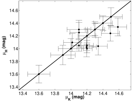
Figure 4: Comparison between the distance modulus obtained with $H$-band data with that obtained with $K$-band data for the same fields. The solid line shows the 1:1 ratio. The two quantities are well correlated and give similar distances.

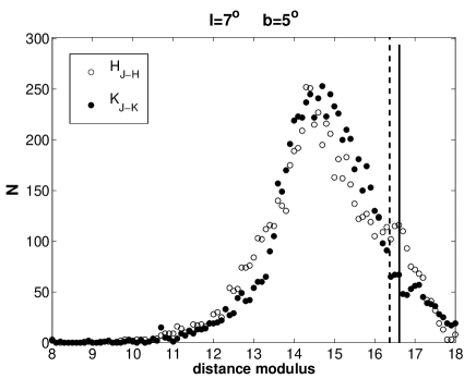
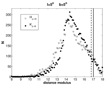
Figure 5: Spatial distribution of red-clump stars obtained with either $H$- or $K$-band corrected magnitudes for the fields $l=7^{\circ}$, $b=5^{\circ}$ (above) and $l=5^{\circ}$, $b=5^{\circ}$ (below). The distributions are very similar, and the maxima are nearly coincident. Vertical lines show the limiting magnitude derived using the $K$ (solid) and $H$ (dashed) bands, respectively.

4 Model fits

The distances to the bar/bulge red-clump cluster of stars are summarized in Table 1 and examples of the fits are shown in Figure 6. Error estimates for the distances have been obtained as a combination of the systematic uncertainties in the intrinsic colour and absolute magnitude of the red-clump population and the fitting error of eq. 2, added in quadrature. The dispersion in distance is represented in each case by $\sigma$. This is estimated from a simple deconvolution:

$$\sigma=\sqrt{\sigma_{\rm RC}^{2}-\sigma_{0}^{2}-\sigma_{e}^{2}},$$ (7)

where $\sigma_{\rm RC}$ is the dispersion of the Gaussian fitted to the histograms by eq. 2, $\sigma_{0}$ is the intrinsic dispersion of the red-clump luminosity, which has been estimated in the range 0.15–0.2 mag (Alves 2000; López-Corredoira et al. 2002) and finally, $\sigma_{e}$ is the photometric error, which for TCS-CAIN is of the order $\sim$0.08 mag (Cabrera-Lavers et al. 2006).

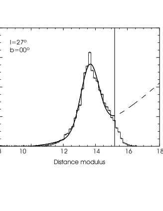
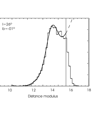
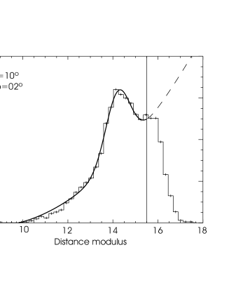
Figure 6: Histograms of the distance modulus in three of the fields used in this work. Fits of eq. 2 to the histograms are shown as solid curves, while vertical lines show the limiting magnitude estimates up to which the fits were performed.

Table 1: Distance modulii and distances derived with the red-clump stars for the 49 fields used along this work, with each field covering 0.07 deg² on the sky centred on the Galactic coordinates given in Cols. (1) and (2). The last eight fields are those in which $H$-band data were used to derive distances.

$l$ (∘)	$b$ (∘)	$\mu$ (mag)	$D$ (kpc)	$\sigma$ (kpc)
18	0.0	14.01$\pm$0.07	6.317$\pm$0.229	0.47
20	0.0	13.68$\pm$0.07	5.449$\pm$0.199	0.44
21	0.0	14.05$\pm$0.09	6.455$\pm$0.298	0.51
22	0.0	13.95$\pm$0.08	6.187$\pm$0.238	0.47
26	0.0	13.81$\pm$0.07	5.778$\pm$0.186	0.41
27	0.0	13.71$\pm$0.08	5.525$\pm$0.216	0.42
28	0.0	13.66$\pm$0.11	5.392$\pm$0.303	0.52
29	0.0	13.62$\pm$0.10	5.308$\pm$0.258	0.50
20	$-$0.5	13.36$\pm$0.08	4.704$\pm$0.184	0.65
20	0.5	13.79$\pm$0.08	5.719$\pm$0.221	0.51
26	$-$0.5	13.58$\pm$0.08	5.211$\pm$0.204	0.52
26	0.5	13.65$\pm$0.12	5.366$\pm$0.304	0.54
27	$-$0.5	13.55$\pm$0.08	5.126$\pm$0.202	0.56
27	0.5	13.72$\pm$0.10	5.536$\pm$0.248	0.49
5	1.0	14.25$\pm$0.07	7.094$\pm$0.217	0.70
6	1.0	14.55$\pm$0.08	8.116$\pm$0.267	0.42
7	1.0	14.15$\pm$0.08	6.767$\pm$0.235	0.67
7	$-$1.0	14.06$\pm$0.07	6.488$\pm$0.206	0.45
8	1.0	14.38$\pm$0.09	7.530$\pm$0.313	0.71
9	1.0	13.97$\pm$0.09	6.236$\pm$0.254	0.62
10	1.0	14.29$\pm$0.10	7.197$\pm$0.332	0.62
15	1.0	13.55$\pm$0.11	5.135$\pm$0.257	0.45
15	$-$1.0	13.33$\pm$0.09	4.626$\pm$0.188	0.54
20	1.0	13.95$\pm$0.12	6.174$\pm$0.365	0.47
20	$-$1.0	13.72$\pm$0.13	5.555$\pm$0.335	0.54
23	1.0	13.49$\pm$0.13	4.991$\pm$0.305	0.58
25	1.0	13.86$\pm$0.11	5.906$\pm$0.322	0.48
25	$-$1.0	13.86$\pm$0.10	5.929$\pm$0.276	0.49
26	$-$1.0	13.51$\pm$0.12	5.028$\pm$0.327	0.56
3	$-$2.0	14.21$\pm$0.07	6.943$\pm$0.229	0.48
5	$-$2.0	14.10$\pm$0.10	6.603$\pm$0.298	0.48
7	2.0	14.08$\pm$0.09	6.542$\pm$0.264	0.54
7	$-$2.0	14.31$\pm$0.10	7.277$\pm$0.333	0.49
10	2.0	14.23$\pm$0.11	7.032$\pm$0.364	0.50
10	$-$2.0	14.36$\pm$0.12	7.444$\pm$0.421	0.55
17	$-$2.0	13.87$\pm$0.15	5.947$\pm$0.441	1.01
1	5.0	14.57$\pm$0.12	8.214$\pm$0.444	0.45
3	5.0	14.28$\pm$0.12	7.185$\pm$0.414	0.46
3	$-$5.0	14.35$\pm$0.12	7.411$\pm$0.390	0.47
5	5.0	14.16$\pm$0.12	6.785$\pm$0.371	0.43
7	5.0	14.04$\pm$0.09	6.430$\pm$0.271	0.72
$-$5	5.0	14.67$\pm$0.11	8.588$\pm$0.459	0.43
$-$3	5.0	14.52$\pm$0.09	8.015$\pm$0.340	0.49
$-$2	5.0	14.56$\pm$0.14	8.183$\pm$0.502	0.48
0	7.5	14.35$\pm$0.13	7.416$\pm$0.415	0.45
5	$-$3.5	14.00$\pm$0.16	6.319$\pm$0.431	0.42
5	3.5	13.72$\pm$0.14	5.549$\pm$0.343	0.44
5	7.5	14.21$\pm$0.14	6.943$\pm$0.524	0.50
10	3.5	13.84$\pm$0.16	5.855$\pm$0.463	0.43

4.1 Contamination from the dwarfs

Although we have used the theoretical traces from the SKY model to isolate the red-clump population to avoid contamination due to other populations in the counts (Fig. 1), there will be some contamination from other sources and the effect of this on the overall shape of the reddening-corrected counts should be estimated. For this, we have used the SKY model to predict the relative number of dwarf stars that will fall into the red-clump region of the CMDs (between the dashed lines in Figure 1). The dwarfs predicted by the SKY model that fell into the red-clump area on the CMD were subtracted from the measured counts to give a new “corrected” distribution. A full description of this procedure can be found in section 3.3.3 of López-Corredoira et al. (2002). What is found is that for $m_{K}<12.5$ only 2.5–5% of the detected sources are dwarfs, but that this rises to 10–40% for $13<m_{K}<14$.

As shown in Fig. 7, both for an in-plane and an off-plane field, there is no significant difference in between the corrected and uncorrected distribution. The effect of dwarfs is more important for fainter magnitudes (hence for apparently more distant sources), so the distributions overestimate the number of sources for higher values of the distance modulus. However, the peak location is dominated by the red-clump population, and any possible contamination does not affect its location. We fitted eq. 2 to the “corrected” distributions and obtained a mean difference in the distance modulus derived from either the uncorrected or corrected data of 0.05 mag (which, translated into distances, yields to a difference of around 100 pc in this case), which is lower than the accuracy of the fit itself. This calculation was done only for a test sample of four randomly selected fields. Since we did not find any significant difference in the results, correction was not attempted for with the remaining fields.

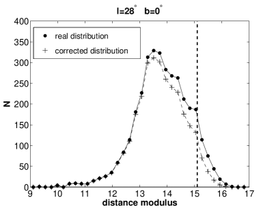
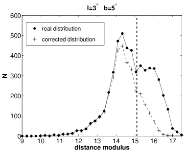
Figure 7: Histograms of the distance modulus for two of the observed fields. Points/solid lines show the histograms derived directly from the data, while dotted/dashed lines show the distributions once corrected for dwarf contamination (using the predictions of the SKY model). Vertical dashed lines stand for the completeness-induced limits for each field.

López-Corredoira et al. (2002) demonstrated that the effect of contamination is more severe off the plane, as extinction helps to separate the populations. The results for off-plane fields show a much better correction of the counts, giving a slightly narrower distribution around the peak. Although applying this could in theory improve the fit, the effect is small and introduces another factor based on models, hence we decided not to apply this correction.

5 The Distribution of sources in the inner Galaxy

5.1 In-plane fields ($|b|<1^{\circ}$)

Results for in-plane fields in the range $18^{\circ}\leq l\leq 29^{\circ}$ show a narrow distribution of distances from the Sun. This is consistent with a high-density feature seen in the red-clump stars with position angle 40$\aas@@fstack{\circ}$5 $\pm$ 3$\aas@@fstack{\circ}$9 (after a linear fit through the points) with respect to the Sun-Galactic Centre direction. First panel in Figure 8 shows the distribution of red-clump density maxima for a face-on view of the Galaxy, with the Galactic Centre at (0,8000 pc). The solid line shows a position angle of 45^∘ (consistent with the 43 degrees given for the bar in Hammersley et al. 2000). The dashed line shows a position angle of 25^∘, which is consistent with the results of Dwek et al. (1995), López-Corredoira et al. (2005), Stanek et al. (1997) and, more recently, Babusiaux & Gilmore (2005). The range of longitudes covered in these fields ($18^{\circ}\leq l\leq 29^{\circ}$), however, is very different from those which obtain the smaller position angle. Only a single point at $l=20^{\circ}$, $b=-0.5^{\circ}$, is observed near the latter position angle. This point could be due to local highly anomalous extinction (see Sect. 5.3), as this line of sight does run close to a major star formation region (Garay et al. 1998; Sridharan et al. 2005). Furthermore, the over-density is is apparently somewhat inhomogeneous, as was noted by Picaud et al. (2003) at $l=20^{\circ}$ and $l=21^{\circ}$.

The gap in the longitude range $23^{\circ}\leq l\leq 25^{\circ}$ is due to the very high extinction that extends up to $|b|\sim 0.4^{\circ}$, which is noticeable also in the mid-infrared range (see Fig. 1 of Benjamin et al. 2005). This makes it impossible to obtain an accurate fit for the fields located in this region. The same problem applies to the in-plane data for $0^{\circ}\leq l\leq 15^{\circ}$. In these fields the completeness limit is far brighter than the apparent magnitude of the K giants for any structure that would be present, that is significantly fainter than the completeness limit. Hence, the above method cannot be applied. However, in the CMD the giant branch from the feature is still visible but its distance cannot be measured.

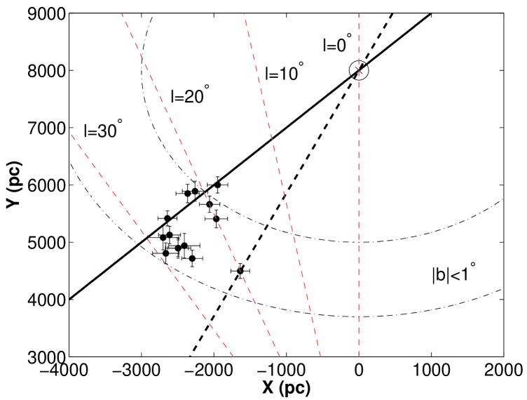
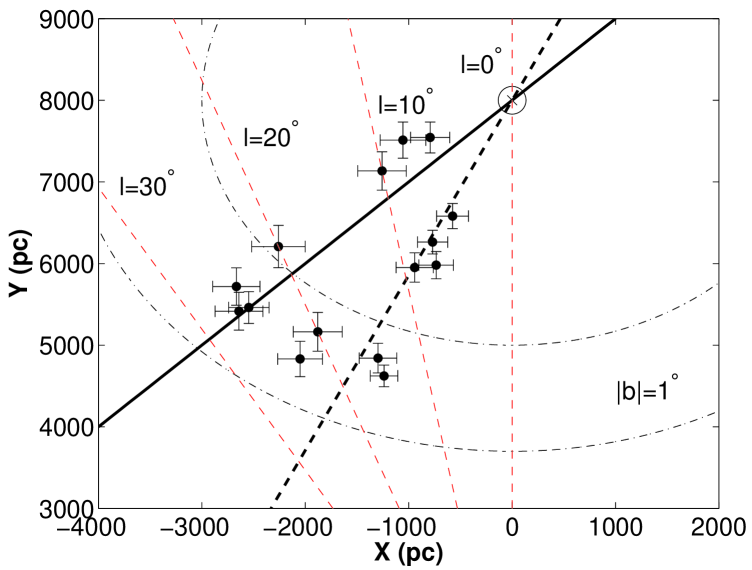
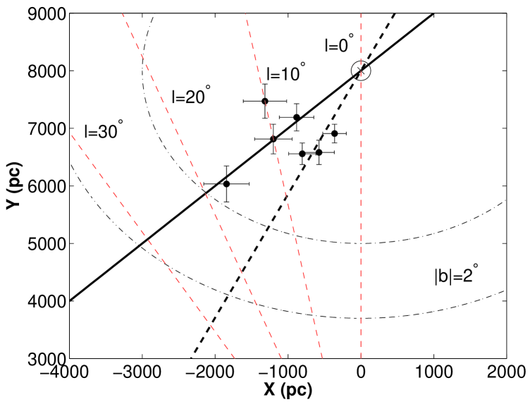
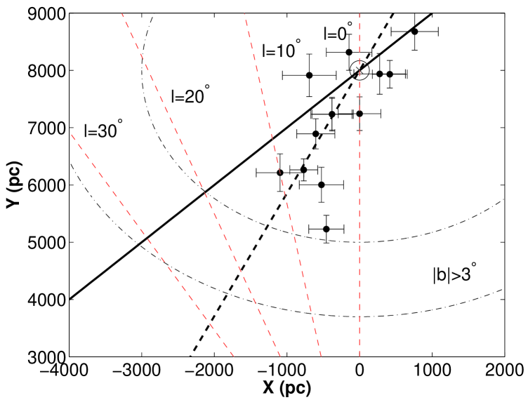
Figure 8: Spatial distribution of red-clump giants maxima in the $XY$-plane at different latitude intervals, with the Sun at (0,0) and the Galactic Center at (0,$8$ kpc) marked with a big circle. Two possible configurations for the observed distribution are also shown: a feature with a position angle of 45^∘ (solid line), and another one with a position angle of 25^∘ (dashed line). Dot-dashed lines define two circles with radii 4.5 kpc and 3 kpc, respectively, while different lines of sight towards the inner Galaxy are also shown in intervals of 10^∘ in longitude. Error bars have been estimated from the distance uncertainties, assuming these divided equally in both the $X$- and $Y$-axes.

5.2 Off-plane fields ($|b|>1^{\circ}$)

The results for $|b|=1^{\circ}$ (second panel in Fig. 8) show that there are two distance regimes for the red-clump population, one that follows approximately the 43$\aas@@fstack{\circ}$4 $\pm$ 3$\aas@@fstack{\circ}$5 angle (nine points) and a second with a smaller angle of 21$\aas@@fstack{\circ}$9 $\pm$ 1$\aas@@fstack{\circ}$0 (six points). Most of the points in this latter feature are at $l<15^{\circ}$, while the points associated with the former are mostly located at $l\geq 20^{\circ}$. Nishiyama et al. (2005) also observed the red-clump stars at $|b|=1^{\circ}$ over the range $8^{\circ}\leq l\leq 15^{\circ}$ and there is good agreement between their distribution of red-clump maxima and ours (Fig. 9), even in the central regions of the Galaxy.

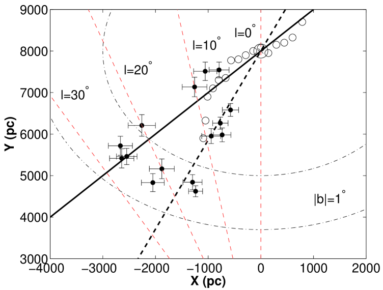
Figure 9: Spatial distribution of red-clump giants maxima presented face on for data at $|b|=1^{\circ}$ and the results obtained for Nishiyama et al. (2005) for comparison (shown as open circles).

For $|b|=2^{\circ}$ the results are less conclusive (third panel in Fig. 8). This is because we are not deep enough to be complete in the red-clump giants in the innermost Galaxy ($|l|<5^{\circ}$) and this makes it difficult to observe the peak in the red-clump counts. Also, for fields $|l|>15^{\circ}$ there is no red-clump cluster observed in the modulus distance histograms, i.e. there is no feature there. Only one point is detected with $l>15^{\circ}$ and this has the highest dispersion in distance of any field. The remainder of the fields lie where there is little difference in distance between the two position angles, making it difficult to clearly assign the red-clump density maxima to one of them. A linear fit to those data yields a global position angle of 36$\aas@@fstack{\circ}$6 $\pm$ 5$\aas@@fstack{\circ}$8 (after discarding those at $l=17^{\circ}$), although if the points are assigned to the position angle that runs closer to that position, and are then averaged separately we obtain position angles of 44$\aas@@fstack{\circ}$1 $\pm$ 2$\aas@@fstack{\circ}$8 and 25$\aas@@fstack{\circ}$1 $\pm$ 2$\aas@@fstack{\circ}$7, respectively.

Farther away from the plane ($|b|>3^{\circ}$) it is possible to sample the innermost Galaxy as the incompleteness effect disappears; however, there are no observable features in the histograms for $l>7^{\circ}$ as the disc component dominates and there is no dense structure at a specific distance. The distribution of red-clump peaks shows in this case a position angle of 30$\aas@@fstack{\circ}$7 $\pm$ 5$\aas@@fstack{\circ}$2 with respect to the Sun–Galactic Centre line (lower panel in Fig. 8). These results are compatible with the position angle of 29^∘ $\pm$ 8^∘ derived in López-Corredoira et al. (2005) for the bulge of the Milky Way using 2MASS data. Also, this result is consistent with the position angle of 22^∘$\pm$5$\aas@@fstack{\circ}$5 recently derived by Babusiaux & Gilmore analysing their private in-plane data at $|l|<10^{\circ}$.

Table 2: Fitted position angles and mean dispersion in distances for the different latitude ranges.

$b$ range	$N$	$\phi_{\rm bar}$ (∘)	$\phi_{\rm bulge}$ (∘)	$\langle\sigma\rangle$ (kpc)
$|b|<1^{\circ}$	14	40.5$\pm$3.9	–	0.48$\pm$0.04
$|b|=1^{\circ}$	15	43.4$\pm$3.5	21.9$\pm$1.0	0.55$\pm$0.09
$|b|=2^{\circ}$	7	44.1$\pm$2.8	25.1$\pm$2.7	0.51$\pm$0.03
$|b|\geq 3.5^{\circ}$	13	–	30.7$\pm$5.2	0.45$\pm$0.02
$|b|=3.5^{\circ}$	3	–	21.6$\pm$3.9	–
$|b|=5^{\circ}$	8	–	31.5$\pm$3.5	–

5.3 The effect of extinction on the results

A global extinction law is assumed when deriving the reddening-independent magnitudes. However, recent results show that there are noticeable differences in the extinction law derived in different directions towards the inner Galaxy (Nishiyama et al. 2006a) and even very small variations in the ratio of total to selective extinction are present on very small scales (Gosling et al. 2006), so care must be taken when applying reddening corrections. The combination of this plus the possible mixture of sources coming from the two position angles would broaden in the distance histograms, hence giving a higher dispersion in distances, $\sigma$.

To examine this effect, we have calculated the mean dispersion in distances in the four latitude ranges showed in Fig. 8 (Table 2). There is clearly less dispersion at $|b|<1^{\circ}$ and at $|b|>3^{\circ}$ than at intermediate latitudes, where the mixture of sources becomes more important (error bars shown in Table 2 account only for the standard deviation of values). The mean values all cluster around 0.5 kpc, but again, with slightly larger values at $|b|=1^{\circ}$ and $|b|=2^{\circ}$. Hence, if we consider the results only for those fields that present $\sigma\leq 0.5$ kpc we obtain the red-clump peak distributions shown in Figure 10.

It is noticeable that in all the cases those points that were originally located at positions intermediate between the two position angles have been removed. Furthermore, only one point has disappeared from the fields at $|b|<1^{\circ}$ and $|b|>3^{\circ}$ as a reflection of the lower dispersion values obtained in those latitude ranges. The point removed is that noted in §5.1 at $l=20^{\circ}$, $b=-0.5^{\circ}$ suggesting that extinction is responsible for its discrepant location.

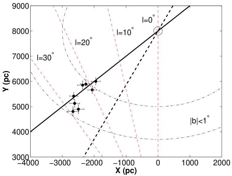
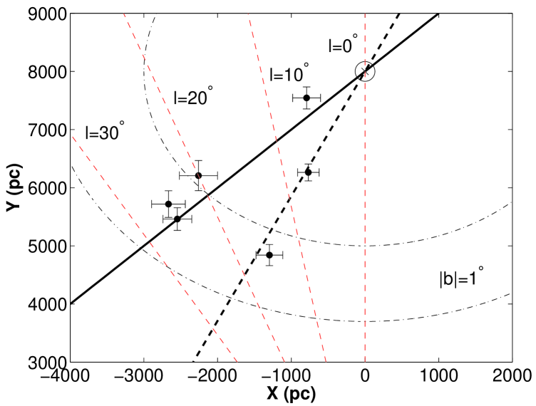
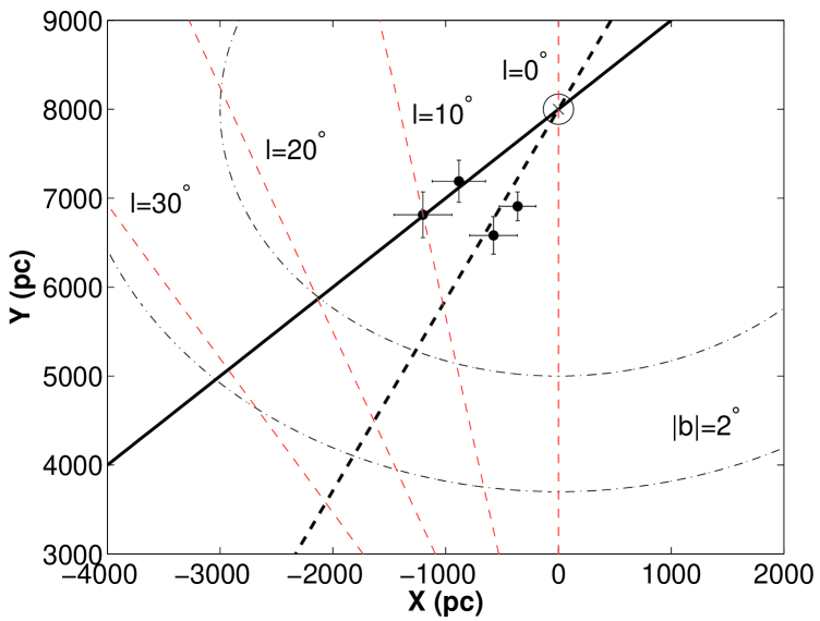
Figure 10: Same as in Fig. 8, but considering only those fields where dispersion in distances is less than 0.5 kpc.

5.4 Discussion of the two position angles

The above shows that:

• The red-clump stars show that there is a dense feature seen on the plane in lines of sight $0^{\circ}<l<28^{\circ}$, but at $|b|>2^{\circ}$ it is only seen for $0^{\circ}<l<10^{\circ}$. In other locations there is no dense feature, and only the disc is seen.

• Away from the Galactic plane for $|l|<10^{\circ}$ the peaks in density of the red-clump population follow a very well defined feature with a position angle of 23$\aas@@fstack{\circ}$1 $\pm$ 0$\aas@@fstack{\circ}$9 with respect to the Sun–Galactic Centre line.

• In the plane ($|b|<1^{\circ}$) for $|l|>18^{\circ}$ there is a longer structure with a distinct position angle of 43$\aas@@fstack{\circ}$0 $\pm$ 1$\aas@@fstack{\circ}$9. This feature is not seen more than 2 degrees away from the plane.

• At intermediate latitudes, there is a mixture of sources coming from both structures producing a more spread out distribution in the distances derived from the red-clump location in the CMDs.

The position angles are derived by a weighted mean of the values summarized in Table 2 for both features.

Sevenster et al. (1999) found a similar effect when comparing $N$-body models with their sample of OH/IR stars and noted that the position angle changed from $\phi$ = 44^∘ when using in-plane fields to $\phi$ = 25^∘ when only high latitude fields were considered. They also noted in the literature that lower values for the viewing angles determined from stellar data were found when low-latitude fields were excluded from the fit, which is in agreement with the work presented here.

The feature seen on the plane $18^{\circ}<l<27^{\circ}$ in the red-clump stars can have no direct link with the Scutum spiral arm. The tangential point to the stars in this arm is at $l\sim 32^{\circ}$, and it would be expected that any features associated with an arm would be strongest there. However, there is no red-clump cluster seen at that location (Hammersley et al. 2000), and inwards of the this point the effect of the arm would become less (Hammersley et al. 1994). Furthermore, a spiral arm would not form a feature that appeared to run directly towards the Galactic Centre.

Extinction can also be discounted. There are a range of extinctions covered between 18${}^{\circ}\leq l\leq 29^{\circ}$ and in no field is the extinction less than is predicted by the simple extinction model used in Wainscoat et al. (1992). In any case, the method used corrects for extinction. Furthermore, our result is in extremely good agreement with the result of Benjamin et al. (2005) (see Fig. 11), where the effects of extinction are significantly reduced. Also, in Fig. 11 we show how the concentration of data seen at $18^{\circ}<l<27^{\circ}$ is not an isolated feature, and how it is consistent with other estimates for this structure obtained with deeper data than ours in different lines of sight to the inner Galaxy. In fact, it is clear that this feature runs to the inner Galaxy, at least up to 1.5-2 kpc from the Galactic Centre, where it merges with the bulge.

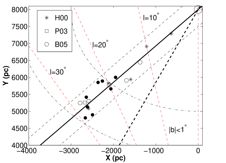
Figure 11: Spatial distribution of red-clump giants maxima for in-plane fields in the $XY$-plane, with some of the more recent estimates for this feature (H00: Hammersley et al. 2000; P03: Picaud et al. 2003; B05: Benjamin et al. 2005). Note there is an excellent agreement between the different sets of data. The long bar with a position angle of 43$\aas@@fstack{\circ}$0 derived in this work is represented by a solid line (and a width of 1 kpc is represented by dashed lines).

The only scenario that readily fits the star count data and CMDs, those presented both here and elsewhere, is that of a triaxial bulge plus a long bar. The bulge has a position angle of about 25^∘ and dominates the counts to $|l|\sim 12^{\circ}$ and up to $|b|=7^{\circ}$ or farther off the plane. The in-plane bar has a position angle of 43^∘ with a half-length of some 4 kpc but is only detected close to the plane. This bulge + bar picture is not so unreasonable. Recent $N$-body simulations on the secular evolution of disc galaxies predict that in a bar-driven evolution, the bar has a thick inner part of shorter extent and a thin outer part of larger extent (Athanassoula 2006), a fact that is in good agreement with observations (Athanassoula 2005; Bureau et al. 2006). Also, the ratio of the thin bar size to the inner bulge length that is derived from our data (between 2.2–2.8 assuming a bulge length of 1.5–2 kpc) is in completely agreement with that was observed in external galaxies (2.7 $\pm$ 0.3, L$\ddot{u}$tticke et al. 2000).

In order to illustrate this, Fig. 12 shows the results from Babusiaux & Gilmore (2005; hereafter BG05). Also shown on the plot are the results from this work and position angles of 45^∘ and 25^∘ degrees. The BG05 data set is deeper than ours (as a result of a pixel scale five times smaller), permitting them to reach the inner Galaxy with in-plane data. It is noticeable that the BG05 points at $l\sim 10^{\circ}$ and $l\sim-5^{\circ}$ coincide with positions for the triaxial bulge obtained here; however, the point at $l\sim-10^{\circ}$ lies on the 45^∘ position angle and is well away from the position required for the triaxial bulge.

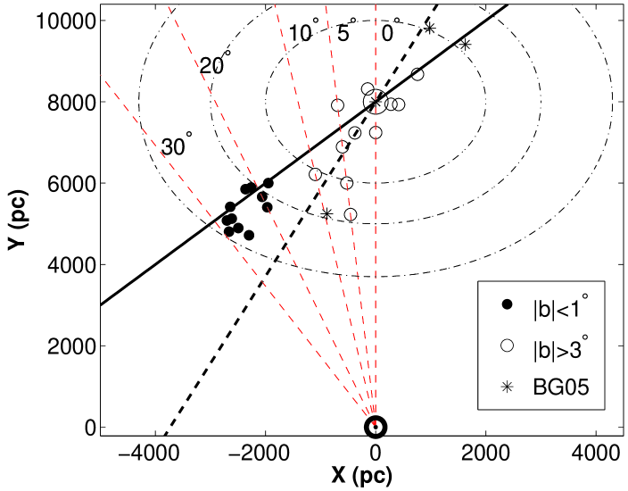
Figure 12: Distribution of positions for the red-clump sources obtained in this work at $|b|<1^{\circ}$ and $|b|>3^{\circ}$ compared with the results of Babusiaux & Gilmore (2005) by using in-plane NIR data. Dot dashed lines delimite circles with radii 4.3 kpc, 3 kpc and 2 kpc, respectively.

5.5 Scale height of bar/bulge sources

From the histograms of the red-clump sources an estimate can be made of the mean scale height of the sources associated with the long thin bar. We have used only those fields with $l\geq 20^{\circ}$ and $|b|\leq 1^{\circ}$, as at $b=2^{\circ}$ there are not sufficient bar sources for a reliable extraction. For each field the space densities along different lines of sight were determined by selecting the stars within one $\sigma$ of the maximum of the histograms of the distance modulus (see Table 1). Combining the distances along the line of sight to the features ($d$) and the Galactic coordinates of the fields ($l,b$) allows these space densities to be expressed with respect to the galactocentric distance ($R$) and the height ($z$) above the plane, taking into account the location of the Sun 15 pc above the mean plane (Hammersley et al. 1995). The result is shown in Figure 13. It can be observed that the mid-point of the distribution is at $z=-41$ pc. Hence, we have represented in Figure 14 the space density with respect to a vertical distance to the plane $z^{*}$, defined as $z^{*}=|z+41|$. This means that the location of this hypothetical long thin bar is $\sim 0.5^{\circ}$ tilted with respect to the mean plane, a result that is compatible with the values found in Picaud & Robin (2004) for the orientation of the outer bulge.

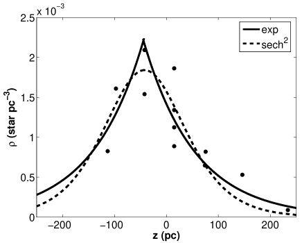
Figure 13: Variation of the space density as a function of distance from the Galactic plane. For comparison, the best fit of an exponential law (solid line) and a sech² law (dashed line) are shown.

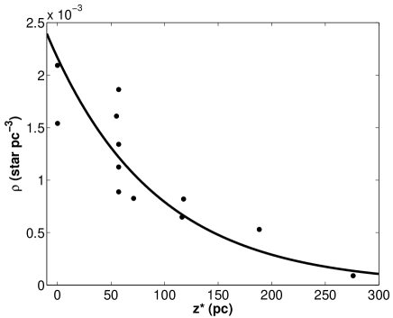
Figure 14: Vertical dependence of the density of bar stars. The best exponential fit, with a scale height of 99.28 $\pm$ 3.13 pc, is also shown as a solid line.

We have also tested a sech² profile to compare with the observed space density for a simple exponential. The two equations used are:

$\rho=\rho_{0}\exp(-z^{*}/h_{z})$,

$\rho=\rho_{0}sech^{2}(z^{*}/h_{z})$

where $h_{z}$ is the scale height of the bar sources and $\rho_{0}$ is the space density in the Galactic plane. The exponential gives $h_{z}$ = 99.3 $\pm$ 3.1 pc and $\rho_{0}$ = 0.022 $\pm$ 0.014 pc^-3, whereas the sech² profile yields $h_{z}$ = 105.4 $\pm$ 5.3 pc and $\rho_{0}$ = 0.018 $\pm$ 0.013 pc^-3. Both fits are shown in Figure 13.

An exponential scale height for the bar of around 100 pc is a factor 2 higher than that previously obtained by López-Corredoira et al. (2001) or Hammersley et al. (1995) from NIR star counts. However, it should be noted that here we are looking at a very different star type than in the previous studies. In both of those cases the stars observed were considerably more luminous, and spectra of a selection of these sources (Garzón et al. 1997) showed that there were a large number of young sources at $l=27^{\circ}$ and $l=21^{\circ}$. The red-clump sources observed here probably represent an older population and hence the larger scale height would be expected. However, the scale height for the red-clump stars in other Galactic components is far higher. For the thin disc it is $\sim$260 pc (Cabrera-Lavers et al. 2005) and applying the same method used above to the bulge for the fields at $|b|\geq 3.5^{\circ}$ gives a scale height of $h_{z}=488\pm 28$ pc (see Fig. 15). Hence the scale height is a further clear indication that on the plane between $18^{\circ}\leq l\leq 29^{\circ}$ there is a geometric component that is very different to the bulge or thin disc.

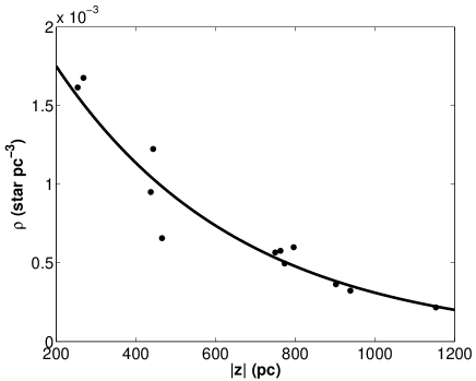
Figure 15: Vertical dependence of the density of inner bulge stars. The best exponential fit shown as a solid line now has a scale height $\sim$5 times higher than that of the thin bar.

6 Systematic uncertainties in the red-clump method

6.1 Deriving distances from the number count histograms

The distances to the red-clump population were obtained by fitting eq. 2 to the distance modulus histograms. However, the maximum of star counts vs. magnitude is not strictly coincident with the maximum in density along the line of sight, which is proportional to the first multiplied by a factor 1/$d^{3}$. Hence the magnitude histogram counts, $N(m)$, should be transformed into density along the line of sight, $\rho(d)$, and eq. 2 then fitted to the resultant distribution. From the relationship between $\rho(d)$ and $N(m)$ it can be shown that the difference between the corrected distance to the maximum in the density distribution ($r^{*}_{m}$) and the distance obtained to the maximum in the counts histograms ($r_{m}$) is:

$$r^{*}_{m}=r_{m}+\Delta r_{m}$$ (8)

$$\Delta r_{m}=\frac{3\leavevmode\nobreak\ \rho(r_{m})}{r_{m}\rho^{\prime\prime}(r_{m})}$$ (9)

$r_{m}$ being the distance to the maximum in the $N(m)$ histogram (hence, $N^{\prime}(m[r_{m}])=0$) and $\rho^{\prime\prime}(r_{m})$ the second derivative of $\rho$ with respect to the distance, measured at $r_{m}$. As $\rho^{\prime\prime}(r_{m})<0$, then $r^{*}_{m}<r_{m}$, thus the corrected distances are slightly lower than those obtained from the maximum of the magnitude histograms.

This effect is more noticeable for the bulge component than for the long thin bar, as $\rho^{\prime\prime}(r_{m})$ is very large for this latter. We have estimated the range of values for $\Delta r_{m}$ for the bulge and for the long bar, obtaining the true density distributions along the line of sight. We have used those fields with $|b|\geq 3.5^{\circ}$ as representative of the bulge, while those in-plane fields with $l>20^{\circ}$ are representative of the long bar. It is found that $\Delta r_{m}$ is in the range 100–300 pc in bulge fields, whereas for long bar fields the effect is far smaller, in the order of 25–50 pc. Figure 16 shows two examples of the change in the overall shape of the density distribution compared to the number count histograms used to derive the distances to the red-clump population. The effect on the determined geometries for either the bulge and the long bar is not large in either case. For the long bar it is ten times lower than the uncertainties in the fit itself (see Table 1) and even for the bulge it is only about 50% of the uncertainty in the fit.

6.2 Difference in maximum density along the line of sight and the position of the major axis of a triaxial structure

The position of the maximum density along the line of sight is not coincident with the the position of the major axis of a triaxial structure unless the structure is very thin along the line of sight (a bar). There are two effects:

• The more important one is that the density along the line of sight reaches a maximum at the tangential point of the innermost ellipsoid along it and this is not in general on the major axis (see Fig. 17).

• For off-plane regions, the lines of sight are not parallel to the $b=0^{\circ}$ and so the larger the distance the greater the height above the plane, and hence the lower the density. Therefore, the maximum density along the line of sight is closer than the real maximum in a plane parallel to $b=0^{\circ}$.

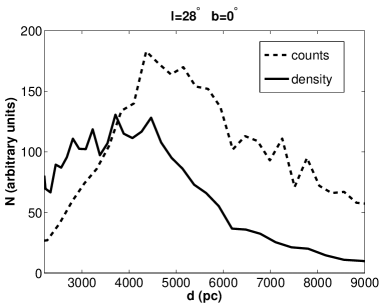
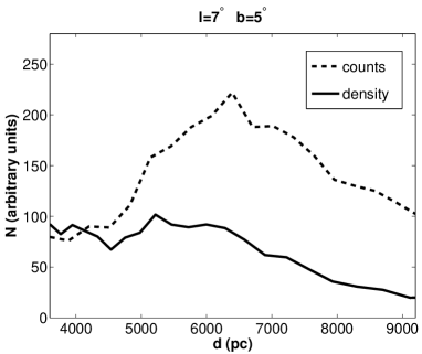
Figure 16: Comparison between the density (solid line) and the number count (dashed line) distributions with respect to the distance along the line of sight for long bar (above) and bulge (below) fields as examples. Density distributions are arbitrarily displaced along the $Y$-axis in order to make both distributions comparable.

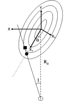
Figure 17: Schematic representation of the difference between the maximum density position along the line of sight (filled square) for triaxial ellipsoids and the intersection of their major axis with the line of sight (filled circle).

We can derive analytically the difference ($\Delta r=r_{m}-r_{a}$) between the maximum density position along the line of sight ($r_{m}$) and the intersection of the line of sight with the major axis ($r_{a}$) for a triaxial structure with monotonically density decreasing outwards. The isodensity contours are defined by the points in space with the same value of $t$:

$$t=\left(x_{1}^{n}+(x_{2}/A)^{n}+(x_{3}/B)^{n}\right)^{1/n},$$ (10)

that in the n=2 case corresponds to isodensity ellipsoids. $A$ and $B$ are the axial ratios of the second and the third axes with respect to the major axis of the ellipsoids, and $x_{i}$ are the Cartesian coordinates with the axis of the ellipsoids concentric with the centre of the Galaxy (see Fig. 17). We assume that the minor axis is perpendicular to the Galactic plane ($x_{3}=z$). $x$, $y$, $z$ are the Cartesian coordinates with $XY$ defining the plane of the Galaxy with the $y$-axis in the Sun–Galactic Centre line and $\alpha$ is the angle between the major axis of the ellipsoid and this $y$-axis (Fig. 17).

The tangential point of the line of sight with the maximum density (filled square in Fig. 17), follows:

$$\frac{\partial t}{\partial r}(r_{m})=0.$$ (11)

Equation 11, together with Eq. 10, lead to

$$x_{1}^{n-1}(r_{m})\frac{\partial x_{1}}{\partial r}(r_{m})+\frac{x^{n-1}_{2}(r_{m})}{A^{n}}\frac{\partial x_{2}}{\partial r}(r_{m})+\frac{x^{n-1}_{3}(r_{m})}{B^{n}}\frac{\partial x_{3}}{\partial r}(r_{m})=0,$$ (12)

which finally lead to

$$\sum_{i=0}^{n-1}\leavevmode\nobreak\ a_{i}\leavevmode\nobreak\ r_{m}^{i}=0,$$ (13)

where

$$a_{n-1}=(-1)^{n}\left(\cos^{n-1}(l+\alpha)+\frac{\tan(l+\alpha)\sin^{n-1}(l+\alpha)}{A^{n}}\right)+$$

$$+\frac{\tan^{n}b}{B^{n}\leavevmode\nobreak\ \cos(l+\alpha)},$$ (14)

and

$$a_{i}=(-1)^{i+1}\left({}^{n-1}_{\leavevmode\nobreak\ \leavevmode\nobreak\ i\leavevmode\nobreak\ }\right)\left(\frac{R_{\odot}}{\cos b}\right)^{n-1-i}\times$$

$$\times\left(\cos^{n-1-i}\alpha\cos^{i}(l+\alpha)+\frac{\sin^{n-1-i}\alpha\sin^{i}(l+\alpha)\tan(l+\alpha)}{A^{n}}\right),$$

$$\forall i\in[0,n-2],$$ (15)

while the position of the major axis (simple geometry with the application of the sine rule, see Fig. 17) is

$$r_{a}=\frac{R_{\odot}}{\cos b}\frac{\sin\alpha}{\sin(l+\alpha)}.$$ (16)

In the simplest case, for $n=2$, Eq. 13 yields

$$r_{m}=\frac{\frac{R_{\odot}}{\cos b}\left[\cos\alpha+\frac{\tan(l+\alpha)\sin\alpha}{A^{2}}\right]}{\cos(l+\alpha)+\frac{1}{A^{2}}\sin(l+\alpha)\tan(l+\alpha)+\left(\frac{\tan b}{B}\right)^{2}\frac{1}{\cos(l+\alpha)}}.$$ (17)

Both of the expressions for $r_{m}$ and $r_{a}$ are coincident for $A\ll$ (very elongated ellipsoids) and $\tan b\ll$ (in the plane), but other cases are affected by a significant systematic error $\Delta r$. Two triaxial structures were examined in order to estimate this effect:

• $A=0.5$, $B=0.4$, $\alpha=28^{\circ}$, typical of the bulge (López-Corredoira et al. 2005): Fig. 18;

• $A=0.11$, $B=0.04$, $\alpha=43^{\circ}$, typical of a long bar: Fig. 19. The low depth in the line of sight of the bar (around 1 kpc) is justifiable because of the low dispersion of the red-clump giants.

The result is that $\Delta r$ is negligible for the bar, with less than $\sim$$150$ pc of systematic error; however, it is not negligible for the bulge, which reaches a discrepancy of up to 1000 pc.

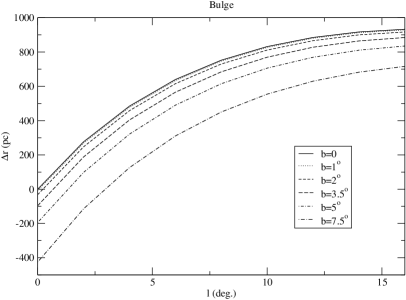
Figure 18: Difference between the maximum density position along the line of sight for triaxial ellipsoids of axial ratios 1:0.5:0.4, oriented with respect to the Sun–Galactic Centre at an angle of 28^∘ (expected for the thick bulge) and the intersection of their major axes with the line of sight.

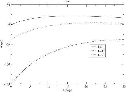
Figure 19: Difference between the maximum density position along the line of sight for triaxial ellipsoids of axial ratios 1:0.11:0.04, orientated with respect to the Sun–Galactic Centre line at an angle of 43^∘ (expected for the long bar) and the intersection of their major axes with the line of sight.

To avoid this effect in deriving the real parameters of the bulge we performed a chi-squared fit to the observed distances of the red-clump density maxima by means of eq. (17), which contains only three free parameters ($A$, $B$ and $\alpha$). We have selected only those points at $|b|>3^{\circ}$, as they are more representative of this component. For each set of model parameters we calculate $\chi^{2}$. Once this was calculated for all sets in the parameter space, we select that one which gives a minimum $\chi^{2}$. Again, for $n=2$ the values which give the minimum $\chi^{2}$ are:

$\alpha=13\aas@@fstack{\circ}$3${}^{+4.7}_{-2.3}$

$A=0.48^{+0.12}_{-0.13}$

$B=0.28^{+0.04}_{-0.03}$

The result for $\alpha$ is notably smaller than that directly derived from the fit to the red-clump density peak, but it is consistent with other estimates found in previous works (Freudenreich 1998; Lépine & Leroy 2000; Picaud & Robin 2004). The axial ratios of the bulge are more or less coincident with those considered in López-Corredoira et al. (2005) and others (e.g. Stanek et al. 1997; Bissantz & Gerhard 2002; Picaud & Robin 2004). It should be noted, however, that eq. 17 is valid only for a series of triaxial ellipsoids, and so will not be correct if the bulge has a different geometry. However, when we use the general formula given by eq. 13 the results do not change noticeably (see Table 3), all of them being compatible with a structure with a position angle of 10–15^∘ (with a weighted mean of 12$\aas@@fstack{\circ}$6 $\pm$ 3$\aas@@fstack{\circ}$2).

Table 3: Parameters derived for different assumed bulge geometries

$n$	$A$	$B$	$\alpha$ (∘)	$\chi_{f}^{2}$	Type
2	0.48${}^{+0.12}_{-0.13}$	0.28${}^{+0.04}_{-0.03}$	13$\aas@@fstack{\circ}3^{+4.7}_{-2.3}$	1.12	ellipsoids
3	0.50$\pm$0.05	0.45$\pm$0.05	10$\aas@@fstack{\circ}2^{+2.8}_{-1.5}$	1.36	—
4	0.55$\pm$0.03	0.45$\pm$0.03	14$\aas@@fstack{\circ}2^{+3.0}_{-3.5}$	4.83	boxy bulge

In summary, the position angle we have derived in this work for the bulge (23$\aas@@fstack{\circ}$1 $\pm$ 0$\aas@@fstack{\circ}$9) by using the distribution of red-clump density maxima might be overestimating the real position angle by around 8–10^∘. So the real position angle of the inner bulge is around 13–15^∘ with respect to the Sun–Galactic Centre line (nearly coincident with the value of 12$\aas@@fstack{\circ}$6 $\pm$ 3$\aas@@fstack{\circ}$2 obtained via chi-squared fitting). In the case of the long thin bar, the effect analysed in this section is less significant and so do not alter the geometry of this component.

7 Confirming the result using 2MASS star counts

The 2MASS survey (Skrustkie et al. 2006) provides a complete coverage of the Galactic Plane in the $JHK_{\rm s}$. Unfortunately, the 2MASS data are not deep enough to reach the red-clump stars in the inner Galaxy, hence the 2MASS data cannot be analysed using the above method. However, the 2MASS star counts can be useful to confirm the proposed morphologies in the inner Galaxy, as they are a powerful tool when searching for asymmetries in the stellar distribution. While the bulge is observed in off-plane regions up to $b\sim 10^{\circ}$ and at $|l|<15^{\circ}$, the long bar is visible only in the in-plane regions, $|b|<2^{\circ}$ and up to $l=27^{\circ}$ at positive longitudes and but only to $l=-15^{\circ}$ at negative longitudes (from the length and position angle). For this study, counts up to $m_{K}$ = 9 mag will be used as this gives a high inner Galaxy-to-disc contrast (Garzón et al. 1993) whilst still providing sufficient sources to give good statistics. A similar analysis was performed in López-Corredoira et al. (2001) with the combination of DENIS (Epchtein et al. 1997) and TMGS (Garzón et al. 1993) $K$-band counts. The advantage of using 2MASS is that it covers the whole region homogeneously and so makes testing the model simpler.

Figure 20 shows the 2MASS star counts with $m_{K}<9$ mag (averaged over $\Delta l=5^{\circ}$) at three different latitude slices: $-0.25^{\circ}<b<0.25^{\circ}$, $-1.25^{\circ}<b<-0.75^{\circ}$ and $-2.25^{\circ}<b<-1.75^{\circ}$. At the distance of the Galactic Centre (7.9 kpc), the heights above the Galactic plane are 0 pc, $-$140 pc and $-$280 pc respectively.

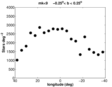
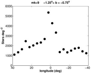
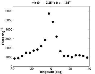
Figure 20: 2MASS star counts with $m_{K}<9$ mag in three different latitude ranges. Counts have been averaged over $\Delta l=5^{\circ}$ to obtain a large number stars in each region, in this way minimizing the Poissonian error.

At $b=0^{\circ}$ there is a large-scale asymmetry about $l=0^{\circ}$ with far more counts at positive longitudes than at negative longitudes. Farther from the plane young inner Galaxy features with very small scale heights should not be significant and the effect of extinction is reduced. Hence, although the contrast with the disc is reduced there should still be sufficient bar counts to see something and the accuracy of model should be massively improved as it cannot deal with the patchy extinction on the plane. In López-Corredoira et al. (2001) it was shown that inner Galactic star counts are more or less symmetric in latitude, with small differences attributed to the Sun being about 15 pc above the Galactic plane (Hammersley et al. 1995) and differences in the extinction above and below the plane. Here, we concentrate our analysis only on those slices at negative latitudes and we assume that the structure of the inner Galaxy is more or less symmetric about the Galactic plane.

We have constructed a very simple Galactic model that includes the contributions of the Galactic disc, a bulge, and a long thin bar to reproduce the 2MASS counts at $\langle b\rangle=-2.0^{\circ}$. For the Galactic disc we have used the luminosity function of Eaton et al. (1984) and an exponential density for the outer Galaxy with a scale height of 285 pc and a scale length of 2.1 kpc (López-Corredoira et al. 2002). The inner 4 kpc of the disc, however, has a constant density (López-Corredoira et al. 2004). It has has been shown that continuing the exponential disc to the Galactic Centre leads to a significant overestimation of the $K$-band star counts (López-Corredoira et al. 2001; Benjamin et al. 2005). This result is consistent with the disc being a Freeman type II disc, which are common in galaxies with long bars. The triaxial bulge has ratios 1:0.5:0.4 and a position angle of the major axis with respect to the Sun–Galactic Centre line of 27^∘ (López-Corredoira et al. 2005). The bulge luminosity function and density law have been also taken from this work. Finally, a simple bar model in agreement with Hammersley et al. (2000) was added. The bar has a depth along the line of sight of 500 pc, a half-length of 4 kpc and a position angle of 43^∘. The distribution was assumed to be constant along the bar, but exponential in height above the plane and the luminosity function used was the same as for the disc although the density was then normalized to make the total counts match those at $l=27^{\circ}$. In all the cases, the extinction model used is as described in Wainscoat et al. (1992).

Whilst the model is simple, it can be shown from Fig. 21 that it does reproduce the counts fairly well at $b=-2^{\circ}$. The model predicts:

• The increasing counts with decreasing longitudes for $|l|>30^{\circ}$ due to the exponential disc

• The sharp jump in the counts at $l=27^{\circ}$ due to the bar

• The basically flat region between $12^{\circ}<|l|<27^{\circ}$ due to exponential disc not continuing into the centre and the bar

• The steep rise inwards of $|l|<10^{\circ}$ as the bulge dominates. The bar/bulge ratio in this region is below 0.025 in this region

There are, however, some other features not well predicted by the simple model. As no ring was included in the model there are excess counts for the region $-30^{\circ}<l<-22^{\circ}$. Sevenster et al. (1999) also observed an excess of OH/IR stars at $l=-22^{\circ}$. The possible implications for an elliptical ring are described in section 6.1 of López-Corredoira et al. (2001) but are beyond the scope of this paper, so will not be repeated here. Similarly, the model does not include the Scutum spiral arm so near the tangential point ($l=33^{\circ}$) there could also be problems. A fuller analysis of the inner Galactic star counts can be found in López-Corredoira et al. (2001; section 3). Here, we are only interested in testing the plausibility of the bulge + thin bar scenario when reproducing the observed counts.

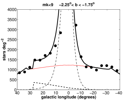
Figure 21: 2MASS star counts to $K<9$ mag and the predictions of a model that includes the contribution of disc (solid line), bulge (dot-dashed line) and a long thin bar (dashed line). The sum of all the components (strong solid line) reproduces the observed counts very accurately.

It is, however, clear from the above that a disc + thin bar + triaxial bulge can account for the a large part of the observed counts, in particular all of the large-scale Galactic features. Were the bar not to be included, the fit would not be as good; in particular the asymmetry in longitude would not be reproduced.

8 Conclusions

By analysing the distribution of red-clump sources along different lines of sight towards the inner Galaxy, we have demonstrated that the Milky Way has two different structures coexisting in the inner $R<5$ kpc: a long thin bar with a half length of 4 kpc constrained to the plane and a position angle of 43^∘, and a thicker bulge with a position angle of 13–15^∘.

In the TCS-CAIN data, each structure dominates at different ranges of longitude and latitude. At $|b|>3.5^{\circ}$, $|l|<10^{\circ}$ the bulge is the only component that is observed whereas at $20^{\circ}<l<28^{\circ}$ and $|b|\leq 0.5^{\circ}$ the long thin bar dominates. The scale heights of these structures are also very different. The red-clump giants of long-bar sources have a scale height of $\sim$100 pc, whereas the disc is over 2.6 times this thick and the bulge sources have a scale height $\sim$5 times larger still. Hence the long bar is geometrically a different structure to the triaxial bulge or disc, although this does not necessarily mean that they are not related.

We have also checked how there are some systematic uncertainties in deriving distances from the red-clump population peaks that have not been taken into account in other similar analyses (e.g. Stanek et al. 1994, 1997; Nishiyama et al. 2005; Babusiaux & Gilmore 2005). Those uncertainties make the position angles derived in those works around 10^∘ larger than the real ones.

We have shown that the large-scale 2MASS star counts in the inner Galaxy can be accurately described by a combination of a triaxial bulge, a bar and a disc. Hence, discussion as to the angle of the bar should be separated into two separate discussions: the form of the triaxial bulge and the form of the long bar.

- (1) Alard, C. 2001, A&A, 379, L44
- (2) Alves D.R., 2000, ApJ, 539, 732
- (3) Athanassoula, E. 2005, MNRAS, 358, 1477
- (4) Athanassoula, E. 2006, astro-ph/0610113
- Athanassoula & Beaton (2006) Athanassoula, E., & Beaton, R. L. 2006, MNRAS, 693
- Beaton et al. (2005) Beaton, R. L., Athanassoula, E., Majewski, S. R., Guhathakurta, P., Skrutskie, M. F., Patterson, R. J., & Bureau, M. 2005, Bulletin of the American Astronomical Society, 37, 1387
- (7) Benjamin, R.A., Churchwell, E., Babler, B.L., et al. 2005, ApJ, 630, L149
- (8) Blitz, L., & Spergel, D.N. 1991, ApJ, 379, 631
- (9) Binney J., Gerhard O. E., & Spergel D. 1997, MNRAS, 288, 365
- (10) Bissantz N., & Gerhard O. E. 2002, MNRAS, 330, 591
- (11) Bonatto, C., Bica., E., & Girardi, L., 2004, A&A, 415, 571
- (12) Bureau, M., Aronica, G., Athanassoula, E., Dettmar, R.-J., et al. 2006, MNRAS, astro-ph/0606056
- Buta et al. (1996) Buta, R., Crocker, D. A., & Elmegreen, B. G. 1996, ASP Conf. Ser. 91: IAU Colloq. 157: Barred Galaxies, 91
- (14) Cabrera-Lavers, A., Garzón, F., & Hammersley, P.L. 2005, A&A, 433, 173
- (15) Cabrera-Lavers, A., Garzón, F., Hammersley, P.L., Vicente, B., & González-Fernández, C., 2006, A&A, 453, 371
- (16) Cohen, M., Hammersley, P.L., & Egan, M.P., 2000, AJ, 120, 3362
- (17) Cole, A.A., & Weinberg, M.D. 2002, ApJ, 574, L43
- (18) de Vaucouleurs, G., 1964, in IAU Symp. 20: The Galaxy and the Magellanic Clouds Interpretation of velocity distribution of the inner regions of the Galaxy, p. 195
- (19) Drimmel, R., Cabrera-Lavers, A., López-Corredoira, M., 2003, A&A, 409, 205
- (20) Duran, M., & van Kerkwijk, M.H. 2006, astro-ph/0606027
- (21) Dwek, E., Arendt, R.G., Hauser, M.G., Kelsall, T., et al. 1995, ApJ, 445, 716
- (22) Eaton N., Adams D. J, Giles A. B., 1984, MNRAS 208, 241
- (23) Epchtein N., 1997, in: The Impact of Large Scale Near-IR Sky Surveys, F. Garzón F., N. Epchtein N., A. Omont, B. Burton, P. Persi, eds., Kluwer, Dordrecht, p. 15
- Freeman (1996) Freeman, K. C. 1996, ASP Conf. Ser. 91: IAU Colloq. 157: Barred Galaxies, 91, 1
- (25) Freudenreich, H. T. 1998, ApJ, 492, 495
- (26) Friedli, D., Wozniak, H., Rieke, M., Martinet, L., & Bratschi, P. 1996, A&AS, 118, 461
- missing (27) Garay, G., Moran, J.M., Rodríguez, L.F., & Reid, M.J. 1998, ApJ, 492, 635
- missing (28) Garzón, F., Hammersley, P.L., Mahoney, T., et al. 1993, MNRAS, 264, 773
- missing (29) Garzón, F., López-Corredoira, M., Hammersley, P.L., Mahoney, T., & Calbet, X. 1997, ApJ, 491, 31
- (30) Gosling, A., Blundell, K., & Bandyopadhyay, R. 2006, astro-ph/0602410
- (31) Grocholski, A.J., & Sarajedini, A., 2002, AJ, 123, 1603
- (32) Hammersley P. L., Garzón F., Mahoney T., Calbet X., 1994, MNRAS 269, 753
- (33) Hammersley P. L., Garzón F., Mahoney T., Calbet X., 1995, MNRAS 273, 206
- (34) Hammersley P.L., Garzón, F., Mahoney, T.J., López-Corredoira, M., & Torres, M.A.P. 2000, MNRAS, 317, L45
- (35) Ibata, R., & Gilmore, G. 1995a, MNRAS, 275, 591
- (36) Ibata, R., & Gilmore, G. 1995b, MNRAS, 275, 605
- (37) Indebetouw, R., et al. 2005, ApJ, 619, 931
- (38) Lépine, J.R.D., & Leroy, P. 2000, MNRAS, 313, 263
- (39) López-Corredoira, M., Cabrera-Lavers, A., Gerhard, O.E. 2005, A&A, 439, 107
- missing (40) López-Corredoira, M., Cabrera-Lavers, A., Gerhard, O., Garzón, F. 2004, A&A, 421, 953
- missing (41) López-Corredoira, M., Cabrera-Lavers, A., Garzón, F., Hammersley, P.L. 2002, A&A, 394, 883
- (42) López-Corredoira, M., Garzón., F., Beckman, J.E., Mahoney, T.J., Hammersley, P.L., & Calbet, X. 1999, AJ, 118, 381
- (43) López-Corredoira, M., Garzón., F., Hammersley, P.L., Mahoney, T.J., & Calbet, X. 1997, MNRAS, 292, 15
- (44) López-Corredoira, M., Hammersley P.L., Garzón, F., Cabrera-Lavers, A., Castro-Rodríguez, N., Schultheis, M., & Mahoney, T.J. 2001, A&A, 373, 139
- (45) López-Corredoira M., Hammersley P. L., Garzón F., Simonneau E., Mahoney T. J., 2000, MNRAS 313, 392
- (46) Ltticke, R., Dettmar, R.-J., & Pohlen, M. 2000, A&A, 362, 435
- (47) Molla, M., Ferrini, F., & Gozzi, G. 2000, MNRAS, 316, 345
- (48) Nikolaev S., & Weinberg M. D. 1997, ApJ, 487, 885
- (49) Nishiyama, S., Nagata, T., Baba, D., Haba, Y., et al. 2005, ApJ, 621, L105
- (50) Nishiyama, S., Nagata, T., Kusakabe, N., Matsunaga, N., et al. 2006a, astro-ph/0601174
- (51) Nishiyama, S., Nagata, T., Sato, S., Kato, D., et al. 2006b, astro-ph/0607408
- missing (52) Picaud, S., Cabrera-Lavers, A., Garzón, F., 2003, A&A, 408, 141
- missing (53) Picaud, S., & Robin, A.C. 2004, A&A, 428, 891
- (54) Pietrzyński, G., Gieren, W.,& Udalski, A. 2003, AJ 125, 2494
- (55) Ramírez, S.V., Stephens, A.W., Frogel, J.A., & DePoy, D.L. 2000, AJ, 120, 833
- (56) Rieke, G. H., & Lebovsky, M. J. 1985, ApJ, 288, 618
- (57) Robin, A.C., Reylé, C., Derriére, S. & Picaud, S. 2003, A&A, 409, 523
- missing (58) Salaris, M., & Girardi, L. 2002, MNRAS 337, 332
- missing (59) Sarajedini, A., Lee, Y.W., & Lee, D.H., 1995, ApJ, 450, 712
- (60) Schultheis, M., Lançon, A., Omont, A., Schuller, F., & Ojha, D.K. 2003, A&A, 405, 531
- (61) Sevenster M., Prasenjit S., Valls-Gabaud D., & Fux R. 1999, MNRAS, 307, 584
- (62) Skrutskie M. F., Cutri, R.M., Stiening R., et al. 2006, AJ, 131, 1163
- (63) Sridharan, T.K., Beuther, H., Saito, M., Wyrowski, F., & Pchilke, P. 2005, ApJ, 634, L57
- Stanek & Garnavich (1998) Stanek, K. Z., & Garnavich, P. M. 1998, ApJ, 503, L131
- (65) Stanek, K.Z., Mateo, M., Udalski, A., Szymański, M., Kaluźny, J., & Kubiak, M. 1994, ApJ, 429, L73
- (66) Stanek, K.Z., Mateo, M., Udalski, A., Szymański, M., et al. 1997, ApJ, 477, 163
- (67) Udalski, A., Symański, M., Kaluźny, J., Kubiak, M., & Mateo. M. 1993, Acta Astron., 43, 69
- (68) Udalski, A., et al. 1994, Acta Astron., 44, 165
- (69) Unavane, M., & Gilmore, G. 1998, MNRAS, 295, 145
- (70) Wainscoat, R. J., Cohen, M., Volk, K., Walzer, H. J., & Schwartz D. E. 1992, ApJS, 83, 111
- (71) Weinberg, M.D., 1992, ApJ, 384, 81