Light tracking through ice and water – Scattering and absorption in heterogeneous media with PHOTONICS

Abstract

In the field of neutrino astronomy, large volumes of optically transparent matter like glacial ice, lake water, or deep ocean water are used as detector media. Elementary particle interactions are studied using in situ detectors recording time distributions and fluxes of the faint photon fields of Cherenkov radiation generated by ultra-relativistic charged particles, typically muons or electrons.

The Photonics software package was developed to determine photon flux and time distributions throughout a volume containing a light source through Monte Carlo simulation. Photons are propagated and time distributions are recorded throughout a cellular grid constituting the simulation volume, and Mie scattering and absorption are realised using wavelength and position dependent parameterisations. The photon tracking results are stored in binary tables for transparent access through ansi-c and c++ interfaces. For higher-level physics applications, like simulation or reconstruction of particle events, it is then possible to quickly acquire the light yield and time distributions for a pre-specified set of light source and detector properties and geometries without real-time photon propagation.

In this paper the Photonics light propagation routines and methodology are presented and applied to the IceCube and Antares neutrino telescopes. The way in which inhomogeneities of the Antarctic glacial ice distort the signatures of elementary particle interactions, and how Photonics can be used to account for these effects, is described.

, url]photonics.tsl.uu.se , , , , , ,

1 Introduction

In optical high energy neutrino astronomy light from particle physics events is observed using a large number of detectors placed deep in glacial ice or in ocean or lake water. Successful simulation and reconstruction of such events relies on accurate knowledge of light propagation within the detector medium. Light propagating through even the clearest water or ice is affected by scattering and absorption. For light sources and receivers separated by distances comparable to the photon mean free path, scattering effects can neither be analytically calculated nor ignored. The typical scattering lengths in these detection media are tens to hundreds of metres. Since this scale is comparable to the typical detector separation, detailed simulation of the photon propagation is required to obtain information necessary for event simulation and reconstruction. The problem is complicated further by the anisotropy of the light emitted in particle interactions and the heterogeneity of detector media. Photonics is a freely available software package [1] containing routines for detailed photon Monte Carlo simulations, which take into account such complexities to provide, in tabulated form, the photon flux distribution throughout a specified medium for an input light source.

With Photonics the photon flux and time distributions can be tabulated for an arbitrarily large volume of a propagation medium, for a user defined range of light source and detector properties. This means that once a Photonics table set has been generated for a class of light sources and detectors, it is possible to quickly and transparently acquire the light yield and time distributions without any need for real-time photon propagation during, for example, particle physics event simulation or reconstruction. This is made possible by the Photonics table reader library, with which a user (program) can dynamically query the pre-calculated tables by specifying the locations and geometrical relations between light sources and detectors. A simulation chain for a complete experimental setup can be achieved by using these interfaces and applying detector specific details such as modelling of electronics, data acquisition, and triggers. For event reconstruction, Photonics provides probability density functions for arrival times of independent photons and the expected number of detected photons.

In this paper we first introduce the relevant physics of the photon propagation (Section 2) and the details of the Photonics implementation (Section 3). We then compare our results with observations of calibration light sources in sea water and glacial ice (Section 4). In Section 5, we present some photon tracking results relevant to the detection of neutrinos with the IceCube neutrino telescope.

2 Light propagation in diffuse media

Our goal was to model the transport of light through glacial ice and water. Photon propagation depends on the optical properties of the medium, in particular on the velocity of light and the absorption and scattering cross sections. Glacial ice is optically inhomogeneous because of depth dependent variations in temperature, pressure, and concentrations of air bubbles and insoluble dust. Since the dust deposits track climatological changes and are therefore assumed to be arranged in horizontal layers, their effect is parameterised as a vertical variation of the optical properties. In addition to this spatial variation, the wavelength dependence of the medium parameters must be taken into account. Before describing the implementation to achieve our goal, we review the optical quantities that must be considered in the simulation, using notation in which the wavelength dependence is left implicit.

The time of light travel is determined by the group velocity of light, which is given by the group refractive index $n_{\mathrm{\mathrm{g}}}$, while various transmission and scattering coefficients depend on the phase velocity [2] and its index of refraction $n_{\mathrm{\mathrm{p}}}$.

Absorption of visible and near UV photons in pure water and ice is due to electronic and molecular excitation processes and is characterised by the absorption length $\lambda_{\mathrm{a}}$. Measurements of light attenuation have been performed at relevant wavelengths in lake water by the Baikal [3] collaboration, and in sea water by the Dumand [4], Nestor [5], Antares [6], and Nemo [7] collaborations. The Amanda collaboration has developed an empirical model for optical absorption in deep glacial ice by combining laboratory and in situ measurements [8].

Photon scattering by scattering centres of general sizes is described by Mie scattering theory [9], which for any wavelength and scattering centre size gives the scattering angle distribution, the phase function. Rahman scattering, where the scattering centre is affected by the scattered photon, and Brillouin scattering, where photons are scattered on (thermal) density fluctuations, may result in a change of photon energy. However, these processes are subdominant to Mie scattering in both glacial ice [10] and sea water [6] where light is scattered by centres of very different types and sizes: from ice crystal point defects to air bubbles and mineral grains in ice, and from biological matter to sediment particles in water.

In natural ice and water it is difficult to determine the phase function from in situ measurements. Instead, the Amanda and Antares collaborations have used calibration light sources to determine the propagation characteristics assuming certain forms of the scattering angle distributions. In the case of ice, a one parameter Henyey-Greenstein (HG) phase function is often used, approximating Mie scattering under the assumption that scattering is forward peaked [11]. For water, a two parameter phase function is more useful. For this paper we mostly use the single parameter HG phase function

$$p_{\mathrm{HG}}(\cos\theta)=\frac{1-\tau^{2}}{2(1+\tau^{2}-2\tau\cos{\theta})^{\frac{3}{2}}},$$ (1)

which is completely characterised by the $\tau$ parameter, the mean of the cosine of the scattering angle $\theta$,

$$\tau\equiv\langle\cos\theta\rangle=\int p_{\mathrm{HG}}(\cos\theta)\cos\theta\,\mathrm{d}(\cos\theta).$$ (2)

The absorption length, $\lambda_{\mathrm{a}}$, and scattering length, $\lambda_{\mathrm{s}}$, are the mean free paths of exponential distributions. The probability density function for the path length $s$ to the next scatter is

$$f_{\lambda_{\mathrm{s}}}(s)\equiv\frac{\mathrm{d}F(s)}{\mathrm{d}s}=\frac{e^{\displaystyle-s/\lambda_{\mathrm{s}}}}{\lambda_{\mathrm{s}}},$$ (3)

where $F(s)$ is the probability distribution function.

When determining ice or water optical properties, there is a degeneracy between $\lambda_{\mathrm{s}}$ and $\tau$. One therefore considers the effective scattering length, $\lambda_{\mathrm{e}}$, defined as

$$\lambda_{\mathrm{e}}=\frac{\lambda_{\mathrm{s}}}{1-\tau},$$ (4)

which in anisotropic scattering is analogous to the (geometric) scattering length $\lambda_{\mathrm{s}}$ in isotropic scattering; it is the distance which light propagates through a turbid medium before the photon directions are completely randomised. Consider a collimated light pulse injected into a non-absorbing medium. In this case, the photons are on average scattered at successive steps of length $\lambda_{\mathrm{s}}$ and the projection of the net velocity vector on the original direction is decreased on average by $\tau=\langle\cos\theta\rangle$ in each scattering step (in which all photons are scattered) [12]. Hence the injected light is effectively transported a forward distance of

$$\lambda_{\mathrm{s}}\sum_{i=0}^{\infty}\tau^{i}\rightarrow\frac{\lambda_{\mathrm{s}}}{1-\tau}=\lambda_{\mathrm{e}},$$ (5)

and $\lambda_{\mathrm{e}}$ has a natural interpretation as the distance that the centre of gravity of the photon cloud advances, in the limit of many scatters.

3 Monte Carlo simulation implementation

In this section we present the main ingredients in our photon Monte Carlo simulation implementation. The end product is a set of photon flux density tables describing the evolution of the light field around a user-defined source. For a given light source, a user-specified large number of photons is generated according to the source characteristics. The photons are then tracked and their contribution to the overall light field is determined and recorded in a cellular grid throughout a user defined portion of space, the simulation volume. The sensor locations are not fixed, but are dynamically specified when accessing the simulation results. The photon intensity and time distributions are stored in a six dimensional binary table. Four of these dimensions are for the spatial and temporal location in the simulation volume with respect to the emission point. As the acceptance of the light sensors is assumed to be azimuthally symmetric, around the vertical axis in heterogeneous media and around any axis in homogeneous media, the photon impact direction is characterised by the zenith angle alone, constituting the fifth dimension. The sixth dimension is the angle from the light source principal axis at which a photon is emitted (this dimension can be used, for example, to reweight the flux tables for a different emission profile). These latter two dimensions are usually integrated over when the photon tables are used with detector simulations. In this case the wavelength and angular sensitivity of the detector elements need to be folded in as the photons are recorded, using recording weights which can be specified in functional or tabular form. For each light source position and orientation one table is produced. A set of tables describes a range of source locations and directions, valid for the specified class of light sources and detectors.

3.1 Media and light source properties

The parameters describing the optical medium ($n_{\mathrm{\mathrm{g}}}$, $n_{\mathrm{\mathrm{p}}}$, $\tau$, $\lambda_{\mathrm{e}}$, $\lambda_{\mathrm{a}}$) are taken to be functions of wavelength and a spatial dimension $Z$, typically specifying the ice or water depth. Thus, the propagation medium is divided into horizontal regions which differ by their optical properties. For media where the single parameter HG approximation does not provide an adequate description of the scattering it can be replaced by other phase functions. An example of this is the treatment of sea water in Section 4.1.

A single simulation run begins with the injection of a photon with wavelength and emission direction chosen from user-specified probability distributions and at a user-specified location. Our procedures support point-like (infinitesimal) light sources, where all emitted photons originate from the same point, and volume light sources where the emission is distributed over a volume. An example light source, essential for neutrino astrophysics, is that of a Cherenkov emitter. In Photonics a Cherenkov emitter is a point-like light source with a Cherenkov wavelength spectrum and an angular emission in a Cherenkov cone [13]. In this case the emission is azimuthally symmetric around the principal axis of the Cherenkov emitter. Closely related are light sources composed of many short Cherenkov emitting tracks, such as electromagnetic cascades. Another category of point-like sources are laser or LED light sources, and in Section 4 we compare our simulation of such sources with observations. Continuous and extended light sources are composed by integration of infinitesimal sources. For example, the light distribution due to a relativistic muon is composed by integrating a series of infinitesimal Cherenkov emitters over space and time, as described in Section 3.4. Simulation results for both point-like and extended Cherenkov emitters are presented in Section 5.

3.2 Coordinate systems for photon flux recording

The Cherenkov light source example possesses cylindrical symmetry. Although this symmetry is typically broken by the response of the propagation medium and the detector, a cylindrical coordinate system aligned with the source’s symmetry axis is a natural choice for the recording of the light flux, and it is therefore used in the following. In addition to cylindrical ($\rho,l,\phi$) coordinates, we have also included functionality to allow the flux to be recorded in spherical ($r,\vartheta,\phi$) or Cartesian ($\varepsilon_{1},\varepsilon_{2},\varepsilon_{3}$) coordinates. A grid over the spatial coordinates defines cells in which the photon flux density and time distributions are averaged. The user-specified region of space covered by these cells constitutes the recording volume.

In some dimensions it can be desirable to have denser binning close to the origin. Therefore, uniform as well as linearly increasing bin sizes are supported for $\rho$, $l$, and the time $t$. In addition to specifying the spatial coordinates where the light flux is recorded relative to the source, the location of the source and the direction of its axis of symmetry with respect to the medium are needed. These can be characterised using just two coordinates, the depth $Z_{\mathrm{s}}$ and the zenith angle $\Theta_{\mathrm{s}}$. This is because of the horizontal symmetry of the medium, as discussed in Section 3.1. Fig. 1 shows the coordinates and a recording cell in which the average flux is recorded.

If in addition to the medium symmetry around $\hat{z}$ we assume that the light source is symmetric with respect to the sign of $\phi$ (besides any light source that is azimuthally symmetric around its axis this is the case for some non-isotropic LED calibration light sources used in glacial ice [8, 14]), the flux needs only to be tabulated for $\phi$ between $0$^∘ and $180$^∘. For heterogeneous media we require that the sensor acceptance and the medium properties are symmetric around the same axis $\hat{z}$. This is not required for homogeneous media since the coordinate system can be rotated make the sensor symmetry axis collinear with the $\hat{z}$ axis used to define source location and orientation. Photonics can be extended to handle cases where the two symmetry axes do not align in heterogeneous media, by adding further dimensions to the photon tables.

Dimension		Bins	Low		High
Radial	${\rho}$	30	0	m	500	m
Longitudinal	${l}$	51	-500	m	500	m
Azimuthal	${\phi}$	10	0	∘	180	∘
Time	${t}$	50	0	ns	6000	ns

Table 1: An example of table binning using cylindrical coordinates. The rotational symmetry of the emitter and the horizontal symmetry of the medium implies an azimuthal symmetry in $\phi$, so that the flux is the same at $-\phi$ and $\phi$.

A binning example is shown in Table 1 for a cylindrical coordinate system. As each single precision floating point number requires four bytes, the size of this example table would be 3 megabytes. To get the total table set size this must be multiplied with the number of light source positions $Z_{\mathrm{s}}$ and zenith angles $\Theta_{\mathrm{s}}$ of interest. For example, with 50 source depths and 20 source angles, the total table set size is 3 gigabytes.

Figure 1: The recording cell geometry with variables used for binning of photon flux data. Photons are emitted from a user-defined light source at $Z_{\mathrm{s}}$ and their flux and time distributions are recorded and averaged in all spatial cells the photons traverse (one of which is shown as a shaded volume). These cells are defined in a coordinate system aligned with the source’s principle axis $\hat{l}$, which is tilted by $\pi-\Theta_{\mathrm{s}}$ with respect to the medium symmetry axis $\hat{z}$. The angle $\phi$ is defined to be zero where the radial vector is maximally aligned with $\hat{z}$. The azimuthal direction $\Phi_{\mathrm{s}}$ is degenerate since the medium properties are assumed to be symmetric around the $\hat{z}$ axis.

3.3 Photon propagation

Starting at their point of origin, the photons are tracked and recorded along straight-line paths between successive scattering points using one of two methods. In the volume-density mode, photons are recorded at equidistant recording points along their paths. In the area-crossing mode, photons are recorded at every surface-crossing into a cell. In the latter mode, the propagation step is dynamically calculated to bring the photon to its next cell boundary. The photon’s propagation properties are always updated at medium boundaries and scattering points, regardless of recording method.

When a scattering point is reached, the photon’s direction is changed by an angle randomly drawn from the selected phase function, typically the HG function in Eq. (1), and in a uniform random azimuthal direction. At this point, the distance to the next scattering point is drawn from an exponentially distributed random variable with a mean value of the local scattering length.

Photon absorption is taken into account by successively updating the photon survival weight $w$ as the photons propagate through regions of different absorption. For a photon tracked $n$ steps, each within a locally homogeneous medium, the weight is given by

$$w=\prod^{n}_{i=0}\exp{\left(-\frac{\Delta s_{i}}{\lambda_{\mathrm{a},i}}\right)},$$ (6)

where $\Delta s_{i}$ is the length of step $i$ in a region with absorption length $\lambda_{\mathrm{a},i}$. The weight is updated every time the photon is scattered, enters a new medium region, or is recorded.

When a photon enters a medium region with different scattering and absorption parameters, these are updated, from ($\lambda_{\mathrm{s}},\lambda_{\mathrm{a}}$) to ($\lambda^{\prime}_{\mathrm{s}},\lambda^{\prime}_{\mathrm{a}}$), at the region boundary. At this point, the remaining distance to the next scatter is $s^{\prime}=s\lambda_{\mathrm{s}}^{\prime}/\lambda_{\mathrm{s}}$, where $s$ would have been the remaining distance to the next scatter in the former region with scattering length $\lambda_{\mathrm{s}}$. Refraction at the boundary is supported but reflection is ignored since it is assumed that refractive index variations are continuous.

During its propagation, the flux contributed by a photon is recorded either in each spatial cell it enters (in area-cossing mode) or each time it completes a propagation step (in volume-density mode). The photon flux $\Phi$ (particles per area and time) at any point $(\rho,l,\phi)$ at a time $T$ after the emission from a light source at a depth $Z_{\mathrm{s}}$ pointing in a direction $\Theta_{\mathrm{s}}$ is denoted $\Phi(Z_{\mathrm{s}},\Theta_{\mathrm{s}},\rho,l,\phi,T-t_{0}(\rho,l))$, where $t_{0}$ is a reference time typically chosen to be the first time causally connected to the light emitted by the source,

$$t_{0}(\rho,l)=\frac{n_{\mathrm{ref}}}{c}\sqrt{\rho^{2}+l^{2}},$$ (7)

where $c$ is the speed of light in vacuum and $n_{\mathrm{ref}}$ is a user-specified reference refractive index. This reference time convention is appropriate for point-like stationary light sources only. For fast moving light sources such as muons a different expression is used which takes into account the more complicated causality condition. The residual time $t\equiv T-t_{0}$ is the time delay caused by scattering, relative to the propagation time for a photon travelling in a straight line. Photons are tracked until their residual times exceed a user-specified value. The tracking of a photon is terminated if it leaves the simulation volume (which can be larger than the recording volume to allow the photon to scatter back into the recording volume) or if its survival weight drops below a pre-set value.

The probability density function for a photon flux at time $t$ is given by

$$f_{\mathrm{pdf}}(Z_{\mathrm{s}},\Theta_{\mathrm{s}},\rho,l,\phi,t)=\frac{\Phi(Z_{\mathrm{s}},\Theta_{\mathrm{s}},\rho,l,\phi,t)}{I(Z_{\mathrm{s}},\Theta_{\mathrm{s}},\rho,l,\phi)},$$ (8)

where $I$ is the time integrated photon flux, or intensity,

$$I(Z_{\mathrm{s}},\Theta_{\mathrm{s}},\rho,l,\phi)=\int_{-\infty}^{\infty}\Phi(Z_{\mathrm{s}},\Theta_{\mathrm{s}},\rho,l,\phi,t)dt.$$ (9)

Since photon fluxes are additive we can determine the time distribution of a combination of light sources through

$$f_{\mathrm{pdf}}(t)=\frac{\sum_{i}I_{i}f_{i}(t)}{\sum_{i}I_{i}}=\frac{\sum_{i}\Phi_{i}(t)}{\sum_{i}I_{i}}.$$ (10)

The way in which the photon intensity in a spatial cell is calculated depends on the recording method. In the area-crossing method, the contribution of each photon to the total flux in the cell depends on the projected surface area of the cell as seen in the direction of the contributing photon as it crosses the cell boundary. In the volume-density method, photons contribute at equidistant recording points along their paths, so that the contribution is proportional to the number of recording points that fall in a given cell. The respective equations for the calculation of the observed intensity, per emitted photon, are

$$I_{\scriptscriptstyle\mathrm{AreaCrossing}} = \frac{1}{N}\sum_{\gamma=1}^{N}w_{\gamma}A_{\bot}^{-1},$$ (11)

$$I_{\scriptscriptstyle\mathrm{VolumeDensity}} = \frac{1}{N}\sum_{\gamma=1}^{N}\sum_{k=1}^{n_{\gamma}}w_{\gamma}(k)\frac{\Delta s}{V},$$ (12)

where the $\gamma$ sum runs over the $N$ simulated photons, $A_{\bot}$ is the recording cell area projected perpendicularly to the direction of the photon, $V$ is the volume of the cell, and $\Delta s$ is the recording point separation along the photon path in the volume-density method. The quantity $n_{\gamma}$ is the number of recording points inside the cell for a given photon. Hence, in the area-crossing mode, photons are recorded at every surface-crossing into a cell, whereas in the volume-density mode, they are recorded at equidistant recording points. The photon weight $w_{\gamma}$ is a product of the absorption-induced survival weight, Eq. (6), and optional user-specified sensor detection efficiencies.

The calculation and recording of a photon’s contribution to the flux in a recording cell is computationally expensive, but a suitable choice of method (area-crossing or volume-density) can speed up the simulation. To optimise for speed one compares the step size $\Delta s$ with the scale dimension of a recording cell $D_{\mathrm{cell}}$. If $\Delta s<D_{\mathrm{cell}}$, the area-crossing method is competitive; otherwise the volume-density method should be used. Hence the area-crossing method can result in faster code execution for large detection volumes with large recording cells, while the volume-density method is faster for small, dense recording cell configurations. To ensure unbiased sampling in volume-density mode even for $\Delta s\gg D_{\mathrm{cell}}$, the path length to the first recording point after emission is drawn from a uniform distribution between 0 and $\Delta s$. To maximise the number of independent sampling points for a given execution time, $\Delta s$ is balanced against the total number of photons $N$. A large $\Delta s$ allows a large $N$, but if too large the number of recordings per execution time will drop as more time is spent propagating photons between recording points. Using $\Delta s\approx\lambda_{\mathrm{s}}$ is often a good compromise.

Another way to improve the speed of the Monte Carlo simulation is through importance-weighted scattering. This means that the photons are propagated using scattering parameters which are different from those of the scattering situation at hand in order to get higher statistics at low probability phase space locations. When solving a Monte Carlo problem for random numbers $x_{i}$ (for example, scattering angles) from a probability density distribution $f_{1}(x)$, we can choose to instead sample from another distribution $f_{2}(x)$ while applying a weight of $f_{1}(x_{i})/f_{2}(x_{i})$. As an example, a user might want to oversample straighter paths to enhance the statistics for early photons at large source-receiver distances. The user could then simply scale the scattering length by a factor $k>1$, propagate photons with scattering described by $f_{k\lambda_{\mathrm{s}}}(s)$ (see Eq. (3)), and reweight each photon by $f_{\lambda_{\mathrm{s}}}(s)/f_{k\lambda_{\mathrm{s}}}(s)$ for every scatter it experiences. Alternatively, the mean cosine of the scattering angle, $\tau$, can be modified to achieve a similar effect using Eq. (4). The effective scattering length is made a factor $k$ longer by $\tau^{\prime}=(k-1+\tau)/k$. The corresponding weight is $f_{\tau}(\theta)/f_{\tau^{\prime}}(\theta)$.

We have described how the photon flux density is calculated in cells throughout the simulation volume. In neutrino astronomy, the quantity of interest is the number of photons detected by an optical sensor such as a photomultiplier. Since the sensor response is usually wavelength and angle dependent but we do not want to store the wavelengths and arrival directions of the simulated photons, Photonics includes the option to fold the sensor response into the simulation when the tables are generated. When this option is selected, user-supplied wavelength and angular efficiency files are used to weight the photon flux density to obtain the detected photon flux.

3.4 Propagating light sources

To this point we have discussed how to obtain a set of tables describing the photon fluxes for a range of locations and orientations of a point-like, stationary light source. A propagating light source can not be satisfactorily approximated as a flash of light from a single spatial point. We discuss in the following the modelling of Cherenkov light from high energy muons, which give rise to kilometre scale Cherenkov emitting tracks in water or ice. Our method, however, applies also to other line-like light sources such as high energy tauons.

To calculate the photon flux distribution generated by a muon we integrate over the photon flux distributions of many point-like Cherenkov emitters with $\Theta_{\mathrm{s}}$ given by the muon direction. A set of point-like photon tables provide the differential light flux $\Phi_{\mathrm{point}}$ at any space-time location from sources at any causally connected location. This serves as integration kernel,

$$G_{\mathrm{point}}(\boldsymbol{x}_{\mathrm{s}}(t_{\mathrm{s}}),\>\boldsymbol{x}_{\mathrm{rec}},t_{\mathrm{rec}})\equiv\frac{\partial}{\partial t_{\mathrm{s}}}\Phi_{\mathrm{point}}(\boldsymbol{x}_{\mathrm{s}}(t_{\mathrm{s}}),\>\boldsymbol{x}_{\mathrm{rec}},t_{\mathrm{rec}}),$$ (13)

where ($\boldsymbol{x}_{\mathrm{s}},t_{\mathrm{s}}$) and ($\boldsymbol{x}_{\mathrm{rec}},t_{\mathrm{rec}}$) are the emission and receiver coordinates. The light distribution of a propagating muon is thus generated by convolving this kernel with the track of the muon, $\boldsymbol{x}_{\mu}(t_{\mu})$, so that

$$\Phi_{\mu}(\boldsymbol{x}_{\mathrm{rec}},t_{\mathrm{rec}})=\int_{t_{\mu_{\mathrm{start}}}}^{t_{\mu_{\mathrm{stop}}}}\!\!G_{\mathrm{point}}(\boldsymbol{x}_{\mu}(t_{\mu}),\>\boldsymbol{x}_{\mathrm{rec}},t_{\mathrm{rec}})\>dt_{\mu}.$$ (14)

Photonics provides the capability to efficiently perform this integration for a series of fixed muon directions and locations and to store the resulting light fluxes in tables like those for the point-like light sources. These tables are then used to obtain the light flux for muon tracks through any part of the simulation volume by interpolation (Section 3.5). Although the construction of muon events through the integration in Eq. (14) can in principle also be done event by event in a detector simulation or event reconstruction, such an approach would often be significantly slower since the number of considered events, and therefore the number of required flux calculations, is typically larger than the number of fixed muon directions and locations needed to adequately cover the relevant range.

To provide the photon flux for any given track length without having to dynamically perform the time consuming integration of Eq. (14), we have developed a scheme based on the subtraction of semi-infinite tracks. The flux at ($\boldsymbol{x}_{\mathrm{rec}},t_{\mathrm{rec}}$) arising from a finite muon starting at $\boldsymbol{x}_{\mathrm{A}}$ and stopping at $\boldsymbol{x}_{\mathrm{B}}$ can be expressed as the difference between two semi-infinite tracks. For two semi-infinite starting tracks, one (denoted $\mu_{\mathrm{A}\rightarrow}$) starting at the point $\boldsymbol{x}_{\mathrm{A}}$ and the other ($\mu_{\mathrm{B}\rightarrow}$) starting at $\boldsymbol{x}_{\mathrm{B}}$ located further along the muon track, we write

$$\Phi_{\mu_{\mathrm{AB}}}(\boldsymbol{x}_{\mathrm{rec}},t_{\mathrm{rec}})=\Phi_{\mu_{\mathrm{A}\rightarrow}}(\boldsymbol{x}_{\mathrm{rec}},t_{\mathrm{rec}})-\Phi_{\mu_{\mathrm{B}\rightarrow}}(\boldsymbol{x}_{\mathrm{rec}},t_{\mathrm{rec}}),$$ (15)

and the probability density function can be written

$$f_{\mu_{\mathrm{AB}}}=\frac{f_{\mu_{\mathrm{A}\rightarrow}}-f_{\mu_{\mathrm{B}\rightarrow}}}{I_{\mu_{\mathrm{A}\rightarrow}}-I_{\mu_{\mathrm{B}\rightarrow}}}$$ (16)

using Eq. (8). This construction of finite tracks is depicted in Fig. 2.

Figure 2: Schematic view of flux tables for four collinear tracks (offset in $x$ for clarity). The light distribution of a finite track (I) is the difference between two semi-infinite tracks (II) and (III). The dotted rectangles show the outer limits of the semi-infinite tables. The gray lines represent example isointensity contours. The representation of photon flux at a point $\boldsymbol{p}_{2}$ far from the starting and stopping points, can be done in two ways. Either, as in (III), by considering the edge of the best matching semi-infinite table, or, as in (IV), with an infinite track table with only a single $l$ bin.

Consider the point $\boldsymbol{p}_{0}$, close to the finite track start point. At this point, the contribution from $\Phi_{\mu_{\mathrm{B}\rightarrow}}$ is comparably small, so that $\Phi_{\mu_{\mathrm{AB}}}\approx\Phi_{\mu_{\mathrm{A}\rightarrow}}$. However, for the point $\boldsymbol{p}_{1}$ close to the end of the finite track, $\Phi_{\mu_{\mathrm{A}\rightarrow}}\approx\Phi_{\mu_{\mathrm{B}\rightarrow}}$ and the calculation of $\Phi_{\mu_{\mathrm{AB}}}$ becomes sensitive to exact numerical cancellation. It is then numerically superior to subtract two semi-infinite stopping tracks, $\mu_{\rightarrow\mathrm{A}}$ and $\mu_{\rightarrow\mathrm{B}}$, and write $\Phi_{\mu_{\mathrm{AB}}}=\Phi_{\mu_{\rightarrow\mathrm{B}}}-\Phi_{\mu_{\rightarrow\mathrm{A}}}$. Our algorithm dynamically chooses between these two descriptions depending on which of the endpoints is closer to the observation point.

For applications in which tracks can be regarded as completely infinite, the flux tables are made smaller by removing redundant information. At a given observation point in the medium, the flux from an infinite muon track with table origin $Z_{1}$, giving the point a longitudinal coordinate $l_{1}$, is identical to the flux in a table with origin $Z_{2}$ where the point is at $l_{2}=l_{1}+(Z_{2}-Z_{1})/\cos\Theta_{\mathrm{s}}$. Therefore in each infinite muon table only one $l$ bin is retained, typically at $l=0$. Fig. 2 illustrates both ways of accessing information about virtually infinite tracks: with infinite tables and with semi-infinite tables.

The size of a set of infinite tables is typically about 1% of the size of the corresponding semi-infinite description, which can be tens of gigabytes. Hence the infinite tables can easily be loaded into computer memory all at once, which is particularly useful in event reconstruction where it can be hard to estimate in advance the properties of an event to be reconstructed. Reconstruction and large table support is discussed in the following section, describing the Photonics reader library.

3.5 Using the photon flux tables for event simulation and reconstruction

For event simulation and reconstruction, the photon flux tables are accessed using either a set of ansi-c procedures, or a more abstract (root compliant) user interface written in c++, both provided with the Photonics package.

The full simulation of for example an ultra relativistic muon crossing the detector volume is performed by first propagating the muon through the detector medium with a charged particle propagator such as MMC [15]. This results in a list of light generating subevents such as minimum ionising muon track segments and associated electromagnetic showers induced by stochastic energy losses. The detector specific simulation program can then query the corresponding Photonics table information to obtain the number and time distribution of detected photons in each detector module from each such subevent. Photonics comes with a variety of idealised light emission profiles, such as those of minimum ionising muons and point-like electromagnetic and hadronic showers.

A set of tables is loaded into memory using the table reader library. The user can then query the photon flux tables by specifying the location ($\boldsymbol{x}_{\mathrm{s}}$) and orientation ($\Theta_{\mathrm{s}},\Phi_{\mathrm{s}}$) of the source, and the location of the light detectors ($\boldsymbol{x}_{\mathrm{rec}}$). Two additional source characteristics are optional in the query: the source length $L$ (applicable to finite muons) and the energy $E$ used to scale the light source intensity. In an experiment simulation, the user first requests the expected number of detected photons $N(\boldsymbol{x}_{\mathrm{s}},\Theta_{\mathrm{s}},\Phi_{\mathrm{s}},\boldsymbol{x}_{\mathrm{rec}},{E},{L})$. This query also returns a table reference which can be used to get photon arrival times randomly drawn from the tabulated time distribution at the corresponding coordinates. For event reconstruction, Photonics also provides the arrival time probability density function $f_{\mathrm{pdf}}(\boldsymbol{x}_{\mathrm{s}},\Theta_{\mathrm{s}},\Phi_{\mathrm{s}},\boldsymbol{x}_{\mathrm{rec}},L,t)$, which can be used by track-fitting algorithms, for example maximum-likelihood routines. Both $f_{\mathrm{pdf}}$ and the photon intensity (giving $N$) are naturally continuous in $L$ and $E$, and are made continuous in $\boldsymbol{x}_{\mathrm{s}},\Theta_{\mathrm{s}},\Phi_{\mathrm{s}},\boldsymbol{x}_{\mathrm{rec}}$, and $t$ by multidimensional linear interpolation. The interpolation of time distributions is flux weighted, in agreement with Eq. (10),

$$f_{\mathrm{pdf}}=\frac{\sum_{i}\omega_{i}I_{i}f_{i}}{\sum_{i}\omega_{i}I_{i}}\textrm{, with\leavevmode\nobreak\ }\textstyle\sum_{i}\omega_{i}=1,$$ (17)

where $\omega_{i}$ are the interpolation weights. When the flux for a requested source direction $\Theta_{\mathrm{s}}$ is interpolated from two surrounding tabulated directions $\Theta_{1}$ and $\Theta_{2}$, these tables are first (implicitly) rotated to $\Theta_{\mathrm{s}}$. The receiver coordinates $\boldsymbol{x}_{\mathrm{rec}}$ are then identical for the $\Theta_{1}$ and $\Theta_{2}$ table. An analogous approach is used for the source origin $\boldsymbol{x}_{\mathrm{s}}$.

It is sometimes necessary to convolve the photon time distributions with the detector time response function or the emission time profile. This can be done with a provided routine operating on the photon flux tables. Convolution with a Gaussian or with one of two light source time distributions with longer positive tails [6] (see Section 4) has been implemented.

Any number of table sets can be loaded simultaneously (limited only by available memory), making it possible to simulate or reconstruct the cumulative signal from different types of light sources (and detectors). This is useful for example when simulating muons with secondary electromagnetic showers from a primary muon track or several coincident muons. Since detailed photon table sets are often many times larger than the primary memory of a computer, we provide some memory management tools. Users can dynamically load and unload tables, and select loading of tables corresponding to limited ranges of depths ($Z_{\mathrm{s}}$) and light source angles ($\Theta_{\mathrm{s}}$). In experiment simulations this is particularly useful since the parameters for the simulated particles are known. In event reconstruction, the loaded tables should cover the phase space taken into account in the fitting algorithms. If memory limitations restrict this phase space, reconstruction can be performed for subregions, on events predetermined to lie within subregions small enough for the corresponding photon tables to fit in memory. Such preselection can be done with a set of more coarsely binned Photonics tables or with other first-guess approaches (for muons, the much smaller tables of the infinite description can be used, see Section 3.4).

In addition to what has already been mentioned, the Photonics package includes several other tools for processing of the photon flux tables, including integration in any dimension and conversion between differential and cumulative time distributions.

4 Comparison with observations

In this section we use measurements with artificial calibration light sources in sea water and glacial ice to demonstrate that Photonics reproduces the general behaviour of the observed photon distributions.

4.1 Modelling of natural water and Antares’ Mediterranean water surveys

The Antares collaboration is constructing a 0.1 km² water neutrino detector in the deep Mediterranean sea  [6]. In the present design the detector has 12 vertical strings, each of which has an instrumented height of about 350 m and consists of 25 storeys with three optical sensors each. Three strings were deployed in 2006 and the remaining strings are scheduled to be installed during 2007.

Absorption and effective scattering lengths in the deep Mediterranean sea water have been investigated by the Antares collaboration [6]. The surveys were performed during several seasons using a calibrated setup of isotropic light sources, one in the blue at 473 nm and one in the UV at 375 nm. For blue (UV) a $\lambda_{\mathrm{a}}$ of 60 (26) m and a $\lambda_{\mathrm{e}}$ of 265 (122) m with 15% time variability are quoted by Antares. The details of the experimental setup, such as the light emission time profile of the source and detector efficiencies, play a large role for the photon flux time distribution profile in media, like ocean water, where scattering is weaker than absorption. In addition, since the light is typically observed at distances shorter than or comparable to the effective scattering length, the scattering phase function plays an even larger role. Antares assumed a weighted sum of a Petzold and a molecular (Einstein-Smoluchowski) distribution. The Petzold distribution has $\tau=0.924$, and is here approximated by a HG distribution, while the molecular distribution is approximated by isotropic scattering (HG with $\tau=0$). Fig. 3 compares our simulation results using this model with Antares measurements from June 2000 [6]. The agreement verifies the validity of the model and our photon flux simulation for this case.

Figure 3: Residual time distributions at two distances from monochromatic flashes in water. The circles and stars are calibration data from ANTARES [6], while the solid curves are our simulation results using the measured water properties. The emission time profiles of the light sources (dashed curves) were measured in air, where scattering and absorption can be ignored. The distributions are normalised to unity at the peak value.

4.2 Modelling of ice and IceCube’s Antarctic glacial ice surveys

The IceCube neutrino telescope, under construction deep in the glacial ice at the geographic South Pole, is planned to become a high-energy neutrino detector of 1 km³ instrumented volume [14]. It is planned to have 80 strings, of which 22 have been deployed as of January 2007, each equipped with 60 encapsulated photomultipliers evenly distributed over depths between 1450 m and 2450 m. IceCube builds on to the 19 strings of the Amanda array, which have been in operation since 2000.

A detailed study of the properties of the deep South Pole glacial ice has been performed by the Amanda collaboration [8]. The glacial ice is very clear in the optical and near UV with absorption lengths of 20–120 m depending on wavelength. At wavelengths shorter than $\sim\!210$ nm and longer than $\sim\!500$ nm, absorption is dominated by the properties of pure ice, while in the intermediate range absorption by impurities dominates. The effective scattering length is on average 25 m, less for shorter wavelengths. Both scattering and absorption are strongly depth dependent and vary on all depth scales. The variations at depths exceeding 1450 m, where bubbles no longer exist, are explained by varying concentrations of insoluble dust deposits which correlate with changes in climatic conditions over geological time scales. By using physics motivated functional forms for the wavelength and depth dependences of scattering and absorption, the Amanda collaboration has elaborated a heterogeneous ice model [8] by investigating a large number of recorded light distributions generated by in situ pulsed and steady light sources at different wavelengths. The resulting effective scattering and absorptions lengths, $\lambda_{\mathrm{e}}$ and $\lambda_{\mathrm{a}}$ as functions of wavelength, were averaged in 10 m depth intervals.

Using the Amanda ice model parameters, we have generated simulated time distributions corresponding to two combinations of wavelength and light source–receiver positions, and compare them with experimental distributions in Fig. 4. The thick solid curves are our results when using the scattering and absorption parameters fitted to these particular delay time distributions [8], with dashed curves representing two opposing deviations within the parameter uncertainty from these fits. The parameters fitted to the displayed distributions were $\lambda_{\mathrm{e}}=27.6$ m, $\lambda_{\mathrm{a}}=20.5$ m for the 532 nm curve, and $\lambda_{\mathrm{e}}=22.6$ m, $\lambda_{\mathrm{a}}=82.0$ m for the 470 nm curve, both with $\tau=0.94$. The slight overestimation in the tail in Fig. 4(b) is due to systematic uncertainties in the simulation of the LED emitter which lead to an imperfect description of the data in this particular case. The thin solid curves are simulation results with the heterogeneous ice model which is based on data from many source–receiver combinations at different depths and wavelengths. The differences between the two solid curves in each picture reflect the fact that the ice model parameters are averages over all fitted parameters in 10 m depth bins and the parameters from individual fits are distributed around these averages.

Figure 4: Residual time distributions for two monochromatic pulsed light sources in deep glacial ice. In (a), light is recorded at a horizontal distance of 75 m from an isotropic laser source located at a depth of 1825 m. In (b), the detector is at a horizontal distance of 140 m from an upward-pointing LED emitter located at a depth of 1580 m. The Amanda calibration data are shown with Poissonian error bars. The intrinsic timing widths of the light sources, less than 10 ns, were not included in the simulation. The thick solid curves are Photonics simulations using the scattering and absorption parameters fitted to these particular time distributions, and the thin dashed curves represent two opposite parameter variations within the parameter uncertainties from the fits. The thin solid curves show our simulation results with the heterogeneous ice model [8].

5 Application to neutrino astronomy

In neutrino astronomy, the universe is studied using high energy neutrinos as cosmic messengers. The neutrinos can be detected optically only after interacting with matter in the vicinity of the neutrino telescope and producing charged, Cherenkov light emitting particles like muons. Some of the emitted light is recorded by optical sensors distributed throughout the detector volume.

Ultra-relativistic muons are the primary channel through which high energy neutrinos are detected by optical neutrino telescopes. They are also the primary background in the form of so-called atmospheric muons arising from high energy cosmic-ray interactions in the Earth’s atmosphere. An extraterrestrial neutrino signal is distinguished from the background of neutrinos and muons created in the atmosphere mainly by differences in energy spectra and angular distributions. It is therefore important to establish the particle energy and direction in every recorded event as accurately as possible. Our software contributes to this aim by providing means for detailed photon flux simulations, using depth and wavelength dependent optical properties as established at a specific site. High-energy neutrino telescopes are typically recording data for several years while they are constructed by adding more optical sensors. Photon flux tables generated by Photonics can cover arbitrarily large volumes and their use is therefore easily scalable to such growing sensor arrays.

To further illustrate the utility of Photonics, we present in this section photon propagation results for the inhomogeneous ice at the site of the IceCube neutrino telescope [8]. The flux in all figures is given per emitted photon, and is weighted with the angular and wavelength dependent acceptance of the optical detectors used by IceCube, so that the figures display the expected number of detections normalised to a 1 m² detection area in the direction of maximum optical module sensitivity. The photon flux tables were also convolved with a 10 ns wide Gaussian to account for photomultiplier jitter.

Fig. 5 shows the photon flux from a simulated infinitesimal electromagnetic cascade at $1730$ m depth ($Z_{\mathrm{s}}=0$ in Amanda detector coordinates). Cascades are initiated in muon energy loss processes as well as in primary neutrino interactions. The light spectra of hadronic and electromagnetic cascades are Cherenkov in nature, but the light originates from many Cherenkov light emitting particles. The Cherenkov emission cone is slightly distorted [16] since not all emitting particles travel in parallel or at the same speed. The cascade in Fig. 5 is oriented toward the surface, at $\Theta_{\mathrm{s}}=135$^∘, pointing at the upper left corner of the picture. A vertical slice through the photon flux containing the principal axis of the light source is displayed. The angular distribution of emitted photons is peaked at the Cherenkov angle, but the photon flux is smoothed out by scattering as it evolves through the ice. After 100 ns, we can still observe a peaked light distribution in the forward direction. At later times, the flux becomes more and more isotropic, to asymptotically resemble that of an isotropic flash.

Since the IceCube sensors are pointing downward they detect upgoing light with a higher efficiency than downgoing light, which needs to be scattered to reach the photomultiplier photocathode. As a result, a point-like light source appears more upward. This can be seen in Fig. 5 where the direction of the light source appears to be oriented at an angle larger than $\Theta_{\mathrm{s}}=135\mbox{${}^{\circ}$}$.

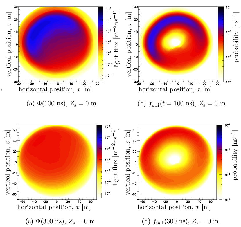
Figure 5: Light flux generated by a simulated electromagnetic cascade near the centre of the Amanda telescope. The upper panel shows a vertical slice of the photon flux (left) and the probability distribution (right) at $t=100$ ns after light emission from a cascade at the origin and oriented toward the upper left at $\Theta_{\mathrm{s}}=135\mbox{${}^{\circ}$}$. The lower panel shows the same distributions at $t=300$ ns. Note the different scales in the two panels.

While the ice is very clear in the centre of the Amanda telescope, there are other depths where stronger scattering and absorption distort the photon flux. In the upper panel of Fig. 6 simulation results are shown for a setup analogous to that of Fig. 5 but with the shower origin 350 m deeper in the ice. This location is immediately below a region of strong scattering and absorption. The cascade direction is again $\Theta_{\mathrm{s}}=135$^∘, but because of the particular medium properties in this region the event shape appears to be more isotropic and even resembles a downward pointing cascade. However, it does differ from truly downward pointing events at the same location, shown in the lower panel of Fig. 6. In this particular case it is exceptionally hard to characterise the event correctly, but by using the correct heterogeneous medium description we improve the possibility to distinguish these cases. This is important for event simulation and reconstruction of parameters such as the zenith angle and the cascade energy.

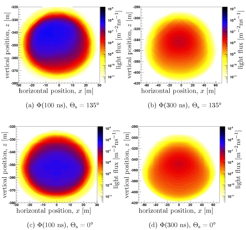
Figure 6: Light fluxes generated by two simulated electromagnetic cascades $350$ m below the Amanda centre. This location is immediately below a region with higher dust concentration that causes stronger scattering and absorption. The flux is shown for both cascades at 100 ns and 300 ns after light emission. Because of the strong scattering and absorption just above the emission point, the flux from the upward pointing ($\Theta_{\mathrm{s}}=135$^∘) source in the upper panel, (a) and (b), evolves from a distribution peaked at the Cherenkov angle to a distribution similar to that from a downward pointing ($\Theta_{\mathrm{s}}=0$^∘) source, shown in the lower panel, (c) and (d).

Inhomogeneities in the detector medium also strongly affect the optical topology of muon events. Fig. 7 shows the light distribution of a simulated muon moving upward through deep South Pole ice. At the front of the track, we observe a cross section of the unscattered Cherenkov wavefront, followed by a diffuse light cloud as the photons are scattered away from the geometrical Cherenkov cone. At depths with higher dust concentrations, photons are obstructed by scattering and absorbed before they can travel very far. This deforms the conical light front, which appears to be bent backwards. In the dusty region near $z=-350$ m, the photon flux is depleted and the surviving photons delayed by increased scattering. Muon track reconstruction is often strongly dependent on the earliest recorded photons, corresponding to the Cherenkov wavefront. Distortions in the wavefront, like in Fig. 7(b), can degrade the reconstruction accuracy unless they are taken into account by the track fitting algorithms.

Fig. 8 shows a snapshot of the light field generated by a finite muon track without secondary interactions. The muon was created at the origin and propagated upward at $\Theta_{\mathrm{s}}=135$^∘ until it decayed after 142 m. The probability density function for such a relatively short track approaches a shape similar to that of point-like cascades, making it hard to distinguish the two cases in an experimental situation with a limited number of points sampled by light sensors. Photonics-based simulations with realistic medium and light source descriptions allow experimentalists to isolate the differences in light profiles for these (and other) distinct cases and to develop appropriate reconstruction algorithms.

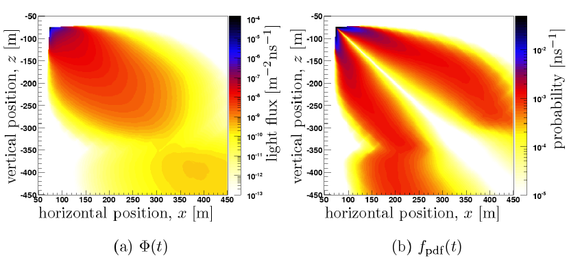
Figure 7: A snapshot of the light field produced by a muon which entered from below, at an angle $\Theta_{\mathrm{s}}=135$^∘. Inhomogeneities in the medium properties distort the smoothly arched light cone, as is most easily seen in the probability density function (b) in the particularly dusty region around $z=-350$ m which has stronger scattering and absorption. In (a), the flux is depleted in the dusty region.

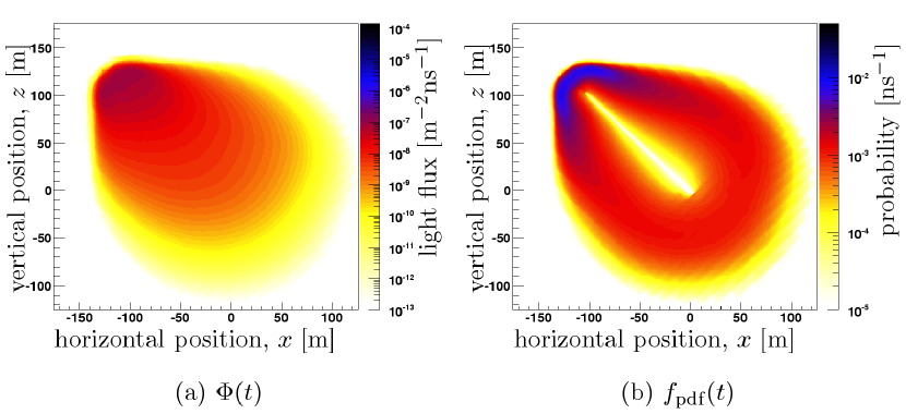
Figure 8: Light distribution from a 142 m long muon track without secondary interactions. This muon was created at the origin and propagated upward at $\Theta_{\mathrm{s}}=135$^∘ until it decayed at $(x,z)=(-100,100)$. The figure shows a snapshot 147 ns after the muon disappeared. Both the photon flux (a) and the probability density function (b) for such a comparably short track are similar to those produced by a point-like cascade.

6 Conclusion

In this paper we have presented the concepts and methods which combine into the Photonics software package. We have explained how the program can be used for calculating and tabulating light distributions around a stationary or moving source, as a function of time and space in scattering and absorbing heterogeneous media. The light distributions obtained from our Monte Carlo simulation agree well with observations of calibration light sources in deep sea water and glacial ice surveys. In the last section it is demonstrated how Photonics can be used to model how optical inhomogeneities of the Antarctic ice at the location of the IceCube neutrino telescope distort the footprints of elementary particle interactions.

7 Acknowledgments

We are grateful to Dr. Nathalie Palanque-Delabrouille for supplying data from the Antares water surveys and her helpful advice on the implementation of water specific parameters. We also thank the members of the Amanda and IceCube collaborations for fruitful discussions and useful feedback.

References

- [1] Photonics, online reference; http://photonics.tsl.uu.se.
- [2] P. B. Price and K. Woschnagg, Role of group and phase velocity in high-energy neutrino observatories, Astropart. Phys. 15 (2001) 97.
- [3] I. A. Belolaptikov et al., Variation of water parameters at the site of the baikal experiment and their effect on the detector performance, Proc. XXIV ICRC, Rome, 1 (1995) 770.
- [4] H. Bradner and G. Blackinton, Long base line measurements of light transmission in clear water, Appl. Optics 23 (1984) 1009.
- [5] E. G. Anassontzis et al., Light transmissivity in the Nestor site, Nucl. Instrum. Meth. A349 (1994) 242.
- [6] J. A. Aguilar et al. (Antares collaboration), Transmission of light in deep sea water at the site of the Antares neutrino telescope, Astropart. Phys. 23 (2005) 131.
- [7] A. Capone et al. (NEMO Collaboration), Measurements of light transmission in deep sea with the AC9 trasmissometer, Nucl. Instrum. Meth. A487 (2002) 423.
- [8] M. Ackermann et al. (Amanda collaboration), Optical properties of deep glacial ice at the South Pole, J. Geophys. Res. 111 (2006) D13203.
- [9] G. Mie, Beiträge zur Optik trüber Medien, speziell kolloidaler Metallösungen, Ann. Phys. 25 (1908) 377.
- [10] P. B. Price and L. Bergström, Optical properties of deep ice at the South Pole: Scattering, Appl. Optics 36 (1997) 4181.
- [11] L. Henyey and J. Greenstein, Diffuse radiation in the galaxy, Astrophys. J. 93 (1941) 70.
- [12] S. Chandrasekar, Radiative transfer, Dover Publications, New York, 1960.
- [13] J. V. Jelly, Cerenkov radiation and its applications, Pergamon Press, London, 1958.
- [14] A. Achterberg et al. (IceCube collaboration), First year performance of the IceCube neutrino telescope, Astropart. Phys. 26 (2006) 155.
- [15] D. Chirkin and W. Rhode, Muon Monte Carlo: a new high-precision tool for tracking of muons in medium, Proc. XXVII ICRC, Hamburg, (2001) 1017.
- [16] C. Wiebusch, The detection of faint light in deep underwater neutrino telescopes, Ph.D. thesis, RWTH Aachen, December 1995, PITHA 95/37.