PROBING THE CLUSTER MASS DISTRIBUTION USING SUBARU WEAK LENSING DATA

Abstract

We present results from a weak lensing analysis of the galaxy cluster A1689 ($z=0.183$) based on deep wide-field imaging data taken with Suprime-Cam on Subaru telescope. A maximum entropy method has been used to reconstruct directly the projected mass distribution of A1689 from combined lensing distortion and magnification measurements of red background galaxies. The resulting mass distribution is clearly concentrated around the cD galaxy, and mass and light in the cluster are similarly distributed in terms of shape and orientation. The azimuthally-averaged mass profile from the two-dimensional reconstruction is in good agreement with the earlier results from the Subaru one-dimensional analysis of the weak lensing data, supporting the assumption of quasi-circular symmetry in the projected mass distribution of the cluster.

Received (Day Month Year)Revised (Day Month Year)

PACS Nos.: include PACS Nos.

1 Introduction

Weak gravitational lensing of background galaxies provides a unique, direct way to study the mass distribution of galaxy clusters.[1, 2] Recent improvements in the quality of observational data usable for lensing studies now allow an accurate determination of the mass distribution in clusters. A1689 is one of the best studied lensing clusters,[3, 4, 5, 6] located at a moderately low redshift of $z=0.183$. Deep HST/ACS imaging of the central region of A1689 has revealed 106 multiply lensed images of 30 background galaxies, which allowed a detailed reconstruction of the mass distribution in the cluster core ($10h^{-1}{\rm kpc}\lower 2.15277pt\hbox{$\;\buildrel<\over{\sim}\;$}r\lower 2.15277pt\hbox{$\;\buildrel<\over{\sim}\;$}200h^{-1}{\rm kpc}$).[3] In Ref. BTU05, we developed a model-independent method for reconstructing the cluster mass profile using azimuthally-averaged weak-lensing distortion and magnification measurements, and derived a projected mass profile of A1689 out to the cluster virial radius ($r\lower 2.15277pt\hbox{$\;\buildrel<\over{\sim}\;$}2h^{-1}$ Mpc) based on the wide-field, deep imaging data taken with Suprime-Cam on the 8.2m Subaru telescope. The combined strong and weak lensing mass profile is well fitted by an NFW[7] profile with high concentration of $c_{\rm vir}\sim 13.7$, which is significantly larger than theoretically expected ($c_{\rm vir}\simeq 4$) for the standard LCDM model.[8]

In this paper we present a weak lensing analysis of A1689 using wide-field Subaru imaging data, with special attention to the map-making process. Throughout this paper, we use the AB magnitude system, and adopt the concordance $\Lambda$CDM cosmology with ($\Omega_{\rm m0}=0.3$, $\Omega_{\lambda 0}=0.7$, $h=0.7$). In this cosmology one arcminute corresponds to the physical scale $129$kpc$/h$ for this cluster.

2 Sample selection

For our weak lensing analysis we used Subaru/Suprime-Cam imaging data of A1689 in $V$ (1,920s) and SDSS $i^{\prime}$ (2,640s) retrieved from the Subaru archive, SMOKA (see Ref. BTU05, Elinor for more details). The FWHM in the final co-added image is $0\hbox{${}^{\prime\prime}$}\!\!.82$ in $V$ and $0\hbox{${}^{\prime\prime}$}\!\!.88$ in $i^{\prime}$ with $0\hbox{${}^{\prime\prime}$}\!\!.202$ pix^-1, covering a field of $30^{\prime}\times 25^{\prime}$. The limiting magnitudes are $V=26.5$ and $i^{\prime}=25.9$ for a $3\sigma$ detection within a $2$^′′aperture. A careful background selection is critical for a weak lensing analysis.[4, 6] For the number counts to measure magnification, we define a sample of 8,907 galaxies ($\bar{n}_{\mu}=12.0$ arcmin^-2) with $V-i^{\prime}>1.0$. For distortion measurement, we define a sample of 5,729 galaxies ($\bar{n}_{g}=7.59$ arcmin^-2) with colors $0.22$ mag redder than the color-magnitude sequence of cluster E/S0 galaxies, $(V-i^{\prime})+0.0209i^{\prime}-1.255>0.22$. The smaller sample is due to the fact that distortion analysis requires galaxies used are well resolved to make reliable shape measurement. We adopt a limit of $i^{\prime}<25.5$ to avoid incompleteness effect. In what follows we will assume $\langle z_{s}\rangle=1$ for the mean redshift of the red galaxies,[3, 4] but note that the low redshift of A1689 means that for lensing work, a precise knowledge of this redshift is not critical.

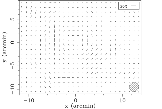
Figure 1: Gravitational reduced-shear field in A1689 obtained from shape distortions of the red background galaxies, smoothed with a Gaussian with ${\rm FWHM}=2^{\prime}$ for visualization purposes. The shaded circle indicates the FWHM of the Gaussian. The coordinate origin is at the optical center (see Figure 4).

3 Lensing Distortions

We use the IMCAT package developed by N. Kaiser to perform object detection, photometry and shape measurements, following the formalism outlined in Ref. KSB. We have modified the method somewhat following the procedures described in Ref. Erben. To obtain an estimate of the reduced shear, $g_{\alpha}=\gamma_{\alpha}/(1-\kappa)$, we measure the image ellipticity $e_{\alpha}$ from the weighted quadrupole moments of the surface brightness of individual galaxies. Firstly the PSF anisotropy needs to be corrected using the star images as references:

$$e^{\prime}_{\alpha}=e_{\alpha}-P_{sm}^{\alpha\beta}q^{*}_{\beta}$$ (1)

where $P_{sm}$ is the smear polarizability tensor being close to diagonal, and $q^{*}_{\alpha}=(P_{*sm})^{-1}_{\alpha\beta}e_{*}^{\beta}$ is the stellar anisotropy kernel. We select bright, unsaturated foreground stars identified in a branch of the half-light radius ($r_{h}$) vs. magnitude ($i^{\prime}$) diagram ($20<i^{\prime}<22.5$, $\left<r_{h}\right>_{\rm median}=2.38$ pixels) to calculate $q^{*}_{\alpha}$.

In order to obtain a smooth map of $q^{*}_{\alpha}$ which is used in equation (1), we divided the $9{\rm K}\times 7.4{\rm K}$ image into $5\times 4$ chunks each with $1.8{\rm K}\times 1.85{\rm K}$ pixels, and then fitted the $q^{*}$ in each chunk independently with second-order bi-polynomials, $q_{*}^{\alpha}(\vec{\theta})$, in conjunction with iterative $\sigma$-clipping rejection on each component of the residual $e^{*}_{\alpha}-P_{*sm}^{\alpha\beta}q^{*}_{\beta}(\vec{\theta})$. The final stellar sample consists of 540 stars, or the mean surface number density of $\bar{n}_{*}=0.72$ arcmin^-2. From the rest of the object catalog, we select objects with $2.4\lesssim r_{h}\lesssim 15$ pixels as an $i^{\prime}$-selected weak lensing galaxy sample, which contains $61,115$ galaxies or $\bar{n}_{g}\simeq 81$ arcmin^-2. It is worth noting that the mean stellar ellipticity before correction is $(\bar{e_{1}}^{*},\bar{e_{2}}^{*})\simeq(-0.013,-0.018)$ over the data field, while the residual $e^{*}_{\alpha}$ after correction is reduced to ${\bar{e}^{*{\rm res}}_{1}}=(0.47\pm 1.32)\times 10^{-4}$, ${\bar{e}^{*{\rm res}}_{2}}=(0.54\pm 0.94)\times 10^{-4}$. The mean offset from the null expectation is $|\bar{e}^{*\rm res}|=(0.71\pm 1.12)\times 10^{-4}$. On the other hand, the rms value of stellar ellipticities, $\sigma_{e*}\equiv\left<|e^{*}|^{2}\right>$, is reduced from $2.64\%$ to $0.38\%$ when applying the anisotropic PSF correction. Second, we need to correct the isotropic smearing effect on image ellipticities caused by seeing and the window function used for the shape measurements. The pre-seeing reduced shear $g_{\alpha}$ can be estimated from

$$g_{\alpha}=(P_{g}^{-1})_{\alpha\beta}e^{\prime}_{\beta}$$ (2)

with the pre-seeing shear polarizability tensor $P^{g}_{\alpha\beta}$. We follow the procedure described in Ref. Erben to measure $P^{g}$. We adopt the scalar correction scheme,[10, 11, 12] namely, $P^{g}_{\alpha\beta}=\frac{1}{2}{\rm tr}[P^{g}]\delta_{\alpha\beta}\equiv P^{g}_{\rm s}\delta_{\alpha\beta}$. The $P_{g}^{\rm s}$ measured for individual objects are still noisy especially for small and faint objects. We remove from the galaxy catalog those objects that yield a negative value of $P_{g}^{\rm s}$ estimate to avoid noisy shear estimates. We then adopt a smoothing scheme in object parameter space.[10, 13, 14] We first identify thirty neighbors for each object in $r_{g}$-$i^{\prime}$ parameter space. We then calculate over the local ensemble the median value $\langle P_{g}^{\rm s}\rangle$ of $P_{g}^{\rm s}$ and the variance $\sigma^{2}_{g}$ of $g=g_{1}+ig_{2}$ using equation (2). The dispersion $\sigma_{g}$ is used as an rms error of the shear estimate for individual galaxies. The mean variance $\bar{\sigma}_{g}^{2}$ over the red galaxy sample is obtained as $\simeq 0.133$, or $\sqrt{\bar{\sigma}_{g}^{2}}\approx 0.36$. Finally, we use the following estimator for the reduced shear: $g_{\alpha}=e^{\prime}_{\alpha}/\left<P_{g}^{\rm s}\right>$.

For map-making, we then pixelize the distortion data into a regular grid of $N_{\rm pix}=21\times 17$ independent pixels, covering a field of $\approx 30^{\prime}\times 24^{\prime}$. The pixel size is $\Delta_{\rm pix}=1\hbox{$.\mkern-4.0mu^{\prime}$}4$, and the mean galaxy counts per pixel is $\sim 15$. The bin-averaged reduced shear is given as $\bar{g}_{\alpha,i}\equiv\bar{g}_{\alpha}(\vec{\theta}_{i})=\sum_{k\in{\rm cell}i}u_{k}g_{\alpha,k}/\sum_{k\in{\rm cell}i}u_{k}$ $(a=1,2;i=1,2,...,N_{\rm pix})$, where $g_{\alpha,k}$ is the estimate of the $\alpha$th component of the reduced shear for the $k$th galaxy, and $u_{k}=1/(\sigma_{g,k}^{2}+\alpha^{2})$ is its inverse-variance weight softened with a constant $\alpha$. Here we choose $\alpha=0.4$.[14] In Figure 1 we show the reduced-shear field obtained from the red galaxy sample, where for visualization purposes the $\bar{g}_{\alpha}(\vec{\theta})$ is resampled on to a finer grid and smoothed with a Gaussian with ${\rm FWHM}=2^{\prime}$.

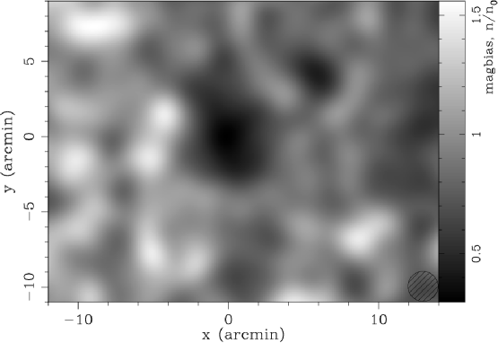
Figure 2: Distribution of the lensing magnification bias $n/n_{0}$ measured from a red-galaxy sample in the background of A1689, smoothed with a Gaussian with ${\rm FWHM}=2^{\prime}$ for visualization purposes. The shaded circle indicates the FWHM of the Gaussian.

4 Magnification Bias

Lensing magnification, $\mu(\vec{\theta})$, influences the observed surface density of background galaxies, expanding the area of sky, and enhancing the flux of galaxies. In the sub-critical regime,[1, 2] the magnification $\mu$ is given by $\mu=1/\left[(1-\kappa)^{2}-\gamma_{1}^{2}-\gamma_{2}^{2}\right]$. The count-in-cell statistics are measured from the flux-limited red galaxy sample (see §2) on the same grid as the distortion data: $N_{i}\equiv N(<m_{\rm cut};\vec{\theta}_{i})=\sum_{k\in{\rm cell}i}1$ with $m_{\rm cut}$ being the magnitude cutoff corresponding to the flux-limit. The normalization and slope of the unlensed number counts $N_{0}(<m_{\rm cut})$ for our red galaxy sample are reliably estimated as $n_{\mu,0}=12.6\pm 0.23$ arcmin^-2 and $s\equiv d\log{N_{0}(m)}/dm=0.22\pm 0.03$ from the outer region $\geq 10^{\prime}$.[4] The slope is less than the lensing invariant slope, $s=0.4$, and hence a net deficit of background galaxies is expected: $N_{i}/N_{0}=n_{\mu,i}/n_{\mu,0}=\mu_{i}^{2.5s-1}$. The masking effect due to bright cluster galaxies is properly taken into account and corrected for.[4] Figure 2 shows a clear depletion of the red galaxy counts in the central, high-density region of the cluster. Note we have ignored the intrinsic clustering of background galaxies, which seems a good approximation,[4] though some variance is apparent in the spatial distribution of red galaxies.

5 Two-Dimensional Mass Reconstruction

The relation between distortion and convergence is non-local, and the convergence $\kappa$ derived from distortion data alone suffers from a mass sheet degeneracy.[1, 2] However, by combining the distortion and magnification measurements the convergence can be obtained unambiguously with the correct mass normalization. Here we combine pixelized distortion and magnification data of the red background galaxies, and reconstruct the two-dimensional (2D) distribution of $\kappa$ using a maximum entropy method (MEM) extended to account for positive/negative distributions of the underlying field.[16, 17] We take into account the non-linear, but sub-critical, regime of the lensing properties, $\kappa$ and $\gamma_{\alpha}$. We take $\kappa_{i}=\kappa(\vec{\theta}_{i})$ as the image to be reconstructed,[16] and express a set of discretized $\kappa$-values as ${\bf p}=\{\kappa_{i}\}$ $(i=1,2,...,N_{\rm pix})$. The total log-likelihood function, $F({\bf p})=-\ln{{\cal L}({\bf p})}$, is expressed as a linear sum of the shear/magnification data log-likelihoods[18] and the entropy term[16]:

$$F({\bf p}) = l_{g}({\bf p})+l_{\mu}({\bf p})-\alpha S({\bf p},{\bf m}),$$ (3)

$$l_{g} \equiv -\ln{{\cal L}_{g}}\approx\sum_{i=1}^{N_{\rm pix}}\sum_{\alpha=1}^{2}\frac{(\bar{g}_{\alpha,i}-\hat{g}_{\alpha,i}({\bf p}))^{2}}{\sigma_{g,i}^{2}},$$ (4)

$$l_{\mu} \equiv -\ln{{\cal L}_{\mu}}\approx\frac{1}{2}\sum_{i=1}^{N_{\rm pix}}\frac{(N_{i}-\hat{N}_{i}({\bf p}))^{2}}{N_{i}},$$ (5)

where $\hat{g}_{\alpha,i}({\bf p})$ and $\hat{N}_{i}({\bf p})$ are the theoretical expectations for $\bar{g}_{\alpha,i}$ and $N_{i}$, respectively, $\sigma_{g,i}\equiv\sigma_{g}(\vec{\theta}_{i})$ is the rms error for $\bar{g}_{i}=\bar{g}_{1}(\vec{\theta}_{i})+i\bar{g}_{2}(\vec{\theta}_{i})$, and $S({\bf p},{\bf m})$ is the cross entropy function for the positive/negative field;[16] the ${\bf m}$ is a set of the model parameters and $\alpha(>0)$ is the regularization constant. The maximum likelihood solution, $\hat{\bf p}$, is obtained by minimizing the function $F({\bf p})$ with respect to ${\bf p}$ for given $\alpha$ and ${\bf m}$. We take $m_{i}={\rm const}\equiv m$, and determine by iteration the Bayesian value of $\alpha$ for a given value of $m$. We found that the maximum-likelihood solution for the Bayesian $\alpha$ is insensitive to the choice of $m$. In the following we set $m$ to be $0.2$. We note that the adopted MEM prior[16, 17] ensures $\kappa_{i}\to 0$ in the noise-dominated regime, $F({\bf p})\sim-\alpha S({\bf p},{\bf m})$ (i.e., maximizing the entropy alone). In order to quantify the errors on the mass reconstruction we evaluate the Hessian matrix of the function $F({\bf p})$ at ${\bf p}=\hat{\bf p}$, $H_{ij}(\hat{\bf p})=\frac{\partial^{2}F({\bf p})}{\partial p_{i}\partial p_{j}}|_{{\bf p}=\hat{\bf p}}$, from which the covariance matrix of the parameters ${\bf p}$ is given by $C_{ij}\equiv\langle\Delta\kappa_{i}\Delta\kappa_{j}\rangle=(H)^{-1}_{ij}(\hat{\bf p})$. Figure 3 displays the $\kappa$ map reconstructed with the MEM method. In Figure 4 we compare the contours of the reconstructed $\kappa$ (thick) and the $i^{\prime}$-band luminosity density of the cluster sequence galaxies (thin) superposed on the $i^{\prime}$-band image of the central region of A1689.

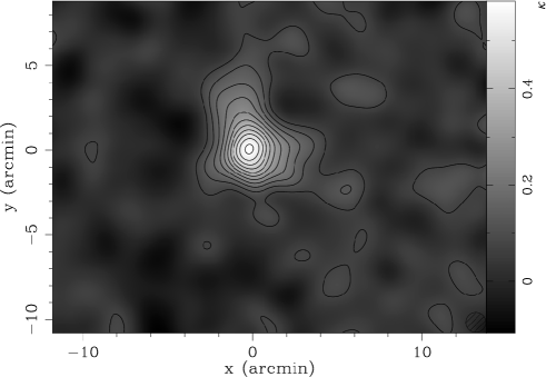
Figure 3: The projected mass distribution $\kappa$ of A1689 reconstructed by a maximum entropy method using weak-lensing distortion and magnification data of red background galaxies. For visualization purposes the $\kappa$-map is resampled on to a finer grid, and smoothed with a Gaussian with ${\rm FWHM}=2^{\prime}$. The lowest contour is $\kappa=0.07$, and the contour steps are $\Delta\kappa=0.05$.

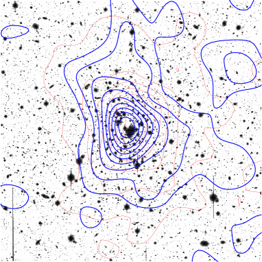
Figure 4: Contours (thick) of the reconstructed lensing convergence $\kappa$ superposed on the $i^{\prime}$-band image of the central region of A1689. The field size is $15^{\prime}$ on a side. The lowest contour and the contour intervals are $0.05$. Also superposed are the contours (thin) of the projected luminosity density of the cluster member galaxies defined by the color-magnitude sequence. North is to the top and East is to the left.

6 Model-Independent Mass Profile of A1689

We show in Figure 5 the azimuthally-averaged profile of the reconstructed convergence, $\kappa(\theta)$, as a function of projected radius $\theta$ from the optical center of A1689 (circles). The vertical error bars represent the $1\sigma$ uncertainties based on the error covariance matrix $C_{ij}$ of the reconstruction. Note that the error bars are correlated. Also shown for comparison are the earlier results from the HST/ACS strong lensing analysis (triangles) and the Subaru weak lensing analysis (squares) with the one-dimensional (1D) reconstruction method, respectively, along with the best-fitting NFW[7] model (solid) for the combined ACS+Subaru profile (see Ref. BTU05).

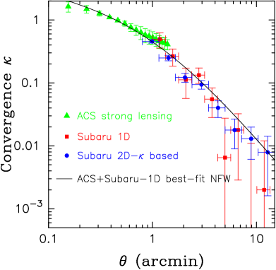
Figure 5: Reconstructed mass profile of A1689. The filled circles with error bars represent the results based on the 2D $\kappa$ map reconstructed with the MEM algorithm. The error bars are correlated. The triangle and square symbols with error bars show the results from the HST/ACS strong lensing analysis (Broadhurst et al. 2005, ApJ, 621, 53) and the Subaru weak lensing analysis with the 1D reconstruction method (Broadhurst, Takada, Umetsu et al. 2005, ApJ, 619, L143, hereafter BTU05) respectively. The solid curve shows the best-fitting NFW profile for the combined ACS+Subaru data by BTU05 ($M_{\rm vir}=1.93\times 10^{15}M_{\odot},c_{\rm vir}=13.7$). The best-fitting NFW profile for the ACS+Subaru profile has a high concentration, $c_{\rm vir}=13.7$, and somewhat overestimates the inner slope and is a bit shallower than the 1D-based results at large radius.

7 Discussion and Conclusions

We presented results from our weak lensing analysis of A1689 based on deep wide-field imaging data taken with Subaru/Suprime-Cam. We used a MEM algorithm to reconstruct the projected mass map in A1689 from combined distortion and magnification data of our red background galaxy sample. The combination of distortion and magnification data breaks the mass sheet degeneracy inherent in all reconstruction methods based on distortion information alone. Our results show that mass and light in A1689 are similarly distributed in terms of shape and orientation, and clearly concentrated around the cD galaxy (see Figure 4). The resulting mass profile from the present full 2D reconstruction is in good agreement with the results from the earlier Subaru 1D analysis[4] (see Figure 5), supporting the assumption of quasi-circular symmetry in the projected mass distribution.

References

- [1] Bartelmann, M. & Schneider, P. 2001, Phys. Rep. 340, 291
- [2] Umetsu, K., Tada, M., & Futamase, T. 1999, Prog. Theor. Phys. Suppl., 133, 53
- [3] Broadhurst, T. et al. 2005, ApJ, 621, 53
- [4] Broadhurst, T., Takada, M., Umetsu, K. et al. 2005, ApJ, 619, L143
- [5] Oguri, M., Takada, M., Umetsu, K., & Broadhurst, T. 2005, ApJ, 632, 841
- [6] Medezinski, E., Broadhurst, T., Umetsu, K. et al. 2007, ApJ in press [astro-ph/0608499]
- [7] Navarro, J. F., Frenk, C. S., White, S. D. M., 1997, ApJ, 490, 493
- [8] Bullock, J. S. et al. 2001, MNRAS, 321, 559
- [9] Kaiser, N., Squires, G., & Broadhurst, T. 1995, ApJ, 449, 460
- [10] Erben, T. et al. 2001, Astron. Astrophys., 366, 717
- [11] Hoekstra, H., Franx, M., Kuijken, K., & Squires, G. 1998, ApJ, 504, 636
- [12] Hudson, M. J., Gwyn, S. D. J., Dahle, H., & Kaiser, N. 1998, ApJ, 503, 531
- [13] Van Waerbeke, L. et al. 2000, Astron. Astrophys., 358, 30
- [14] Hamana, T. et al. 2003, ApJ, 597, 98
- [15] Bertin, E., & Arnouts, S. 1996, Astron. Astrophys. Suppl., 117, 393
- [16] Maisinger, K., Hobson, M. P., & Lasenby A. N. 1997, MNRAS, 290, 313
- [17] Hobson, M. P. & Lasenby, A. N. 1998, MNRAS, 298, 3, 905
- [18] Schneider, P., King, L., & Erben, T. 2000, Astron. Astrophys., 353, 41