Multisite campaign on the open cluster M67. II. Evidence for solar-like oscillations in red giant stars

Abstract

Measuring solar-like oscillations in an ensemble of stars in a cluster, holds promise for testing stellar structure and evolution more stringently than just fitting parameters to single field stars. The most ambitious attempt to pursue these prospects was by Gilliland et al. (1993) who targeted 11 turn-off stars in the open cluster M67 (NGC 2682), but the oscillation amplitudes were too small ($<20\,\mu$mag) to obtain unambiguous detections. Like Gilliland et al. (1993) we also aim at detecting solar-like oscillations in M67, but we target red giant stars with expected amplitudes in the range 50–500$\,\mu$mag and periods of 1 to 8 hours. We analyse our recently published photometry measurements, obtained during a six-week multisite campaign using nine telescopes around the world. The observations are compared with simulations and with estimated properties of the stellar oscillations. Noise levels in the Fourier spectra as low as $27\,\mu\mathrm{mag}$ are obtained for single sites, while the combined data reach $19\,\mu\mathrm{mag}$, making this the best photometric time series of an ensemble of red giant stars. These data enable us to make the first test of the scaling relations (used to estimate frequency and amplitude) with an homogeneous ensemble of stars. The detected excess power is consistent with the expected signal from stellar oscillations, both in terms of its frequency range and amplitude. However, our results are limited by apparent high levels of non-white noise, which cannot be clearly separated from the stellar signal.

1 Introduction

The first clear detection of solar-like oscillations in a red giant star ($\xi\,\mathrm{Hya}$; Frandsen et al., 2002; Stello, 2002) opened up a new part of the Hertzsprung-Russell diagram to be explored with asteroseismic techniques. Following that discovery, detailed analysis of $\xi\,\mathrm{Hya}$ has been performed (Teixeira et al., 2003; Stello et al., 2004, 2006) and new discoveries of oscillations in similar stars have emerged ($\varepsilon\,\mathrm{Oph}$ and $\eta\,\mathrm{Ser}$; Barban et al., 2004; De Ridder et al., 2006). These results are all based on radial velocity measurements of high precision ($\sigma\sim 2\,$m/s) but from non-continuous observations, which imposes large ambiguities on the results (Stello et al., 2006; De Ridder et al., 2006). With oscillation periods of a few hours, these stars require a time base of roughly one month, which can only be obtained on small telescopes. But the current lack of high-precision spectrographs on small telescopes makes a multisite campaign impossible.

However, using photometry makes it feasible to incorporate many 1–2m class telescopes in a multisite campaign, and it furthermore provides the possibility to observe many stars, like in a cluster, simultaneously. Detecting oscillations in a set of cluster stars potentially increases the power of the asteroseismic measurements due to the additional constraints provided by the common parameters of the cluster members (age and composition). Until recently, there has been no such ground-based photometric campaign aimed at detecting solar-like oscillations in red giant stars. A number of attempts have been made to detect oscillations in more Sun-like stars (hotter and less luminous) of the open cluster M67 (Gilliland & Brown, 1988; Gilliland et al., 1991; Gilliland & Brown, 1992), with the most ambitious multisite effort made by Gilliland et al. (1993). Despite noise levels as low as $0.29\,\mathrm{mmag}$ per minute integration no unambiguous detections were claimed. In a recent paper (Stello et al., 2006,  hereafter Paper I), we reported observations from a large six-week multisite campaign also aimed at M67. However, unlike the previous studies our campaign was optimized for the slightly brighter and longer period red giant stars (see Fig. 1), and also covered a much longer time span. The long oscillation periods mean that non-white noise such as drift is more crucial for this project than in the previous studies. The data set reported in Paper I was based on very different sites, many with unknown long-term stability performances. A realistic estimate of the final non-white noise in the data could therefore not be obtained prior to observations.

In this paper our main emphasis is on the time series analysis of the red giant stars (Sect. 4), based on the data described in Paper I. We report in Sect. 2 on an additional independent data reduction method to further obtain lower noise in the Fourier spectra. In Sect. 3 we estimate the oscillation characteristics and simulate in Sect. 5 the expected outcome for each target without the presence of non-white noise to facilitate the analysis of the observations. We give our conclusions in Sect. 6.

Figure 1: Colour-magnitude diagram of the open cluster M67 (photometry from Montgomery et al., 1993). The target stars are indicated with identifier numbers corresponding to those given in Tables LABEL:tab2 and LABEL:tab4. The solid line is an isochrone with $(m-M)=9.7\,\mathrm{mag}$, $\mathrm{Age}=4.0\,\mathrm{Gyr}$, $Z=0.0198$ and $Y=0.2734$ from the BaSTI database (Pietrinferni et al., 2004).

2 Observations and data reduction

The data are from a global multisite observing campaign with nine 0.6-m to 2.1-m class telescopes from 6 January to 17 February 2004 (Paper I). The photometric time series of those stars within the field-of-view of all telescopes comprises roughly 18000 data points.

After calibrating the CCD images we used the MOMF package (Kjeldsen & Frandsen, 1992), which calculated differential time series of 20 red giants relative to a large ensemble of stars (from 116 to 358 stars, depending on telescope field-of-view). We performed the following three initial steps to improve the signal-to-noise in the final Fourier spectra of the time series: (1) sigma clipping, (2) correction for colour extinction and (3) calculation of weights for each data point. For further details see Paper I.

In addition to the time series produced by D.S., as described above, H.B. constructed differential time series following the approach of Honeycutt (1992). This was based on the raw time series (also calculated by MOMF), but using only the red giant stars as the ensemble. For each target star, the differential time series was calculated by subtracting a reference time series that did not include the star itself. The reference time series comprised offsets for each data point (CCD image), which were a weighted average of the ensemble. For each data point the weight $w$ given to each star was calculated as $w=1/(\sigma_{\mathrm{ptp}}+\sigma_{\mathrm{min}})$, where $\sigma_{\mathrm{ptp}}$ is the local point-to-point scatter and $\sigma_{\mathrm{min}}=1\,$mmag is a fixed minimum noise value to prevent a single star with very low noise from dominating the ensemble. Using the relatively small homogeneous ensemble comprising only red giants has the advantage of better removing colour-dependent extinction, and hence providing a lower noise level in the Fourier spectrum at low frequencies. However, simulations showed that the reference time series will include stellar oscillations with amplitudes up to 30% of those we want to detect. The stars with the longest periods (hence largest amplitudes) will be the most affected because the sample is dominated by these.

In most stars, the two methods produced very similar noise levels in the time series, within 10%. However, on a few stars differences of up to 50% were seen. In the following, we chose the time series for each star and each site with the lowest noise in the Fourier spectrum in the interval 300–900$\,\mu$Hz, which is outside the frequency range where the stars are expected to oscillate.

Table 1: Properties of red giant target stars.

No	$V$	$B-V$	$L/\mathrm{L}_{\sun}$	$T_{\mathrm{eff}}$	$\delta L/L$ $\mu$mag			$\nu_{\mathrm{max}}$	$\Delta\nu_{0}$	Cross-ref		P
	mag	mag		K	$(L/M)$	$(L/M)^{0.7}$		$\mu$Hz	$\mu$Hz			%
3	9.72	1.37	250.6	3920	2080	434		3.7	0.7	S978/	G8	53/95
11	9.69	1.36	243.5	3960	1980	417		3.9	0.8	S1250/	G4	58/95
4	10.30	1.26	87.0	4330	592	170		15.1	2.2	S1016/	G5	78/93
21	10.47	1.12	51.9	4727	296	99		34.4	4.2	S1592/		48/92
8	10.48	1.11	50.8	4750	287	97		35.8	4.3	S1010/	G2	82/96
9	10.48	1.10	50.2	4772	281	95		36.8	4.4	S1084/		80/92
10	10.55	1.12	48.2	4727	275	94		37.0	4.4	S1279/	G7	79/92
20	10.55	1.10	47.1	4772	264	91		39.2	4.6	S1479/		76/95
2	10.59	1.12	46.4	4727	265	92		38.4	4.6	S1074/		74/91
18	10.58	1.10	45.8	4772	256	89		40.3	4.7	S1316/		73/95
16	10.76	1.13	40.3	4703	232	84		43.5	5.0	S1221/		92/90
5	11.20	1.08	25.4	4815	140	58		74.8	7.6	S1054/	G9	93/64
17	11.33	1.07	22.4	4835	122	53		86.0	8.4	S1288/		94/96
7	11.44	1.06	20.2	4854	109	49		96.9	9.2	S989/	G12	95/95
19	11.52	1.05	18.7	4873	101	46		106.0	9.9	S1254/		94/95
15	11.63	1.05	16.9	4873	91	43		117.3	10.6	S1277/		95/95
14	12.09	1.01	11.2	4945	58	31		187.3	15.2	S1293/		96/93
12	12.11	1.01	11.0	4947	57	31		190.2	15.4	S1264a/	G15	0/75
13	12.23	0.99	9.9	4966	51	28		213.2	16.8	S1305/		96/95
6	12.31	0.99	9.2	4971	48	27		230.2	17.8	S1103/		95/—

3 Expected oscillation signal

To better interpret our results, we have estimated the characteristics of solar-like oscillations expected in the red giant stars. We scaled the oscillation parameters of the Sun to predict amplitude, central frequency of excess power and the large frequency separation. These predictions are used in Sects. 4 and 5 to compare with the observations.

The predicted amplitude in the Johnson $V$ filter ($\lambda_{\mathrm{cen}}=544\,\mathrm{nm}$) was derived using the scaling relation by Kjeldsen & Bedding (1995) (using $1\,\mathrm{ppm}=1.086\,\mu$mag):

$$(\delta L/L)_{\lambda}={L/\mathrm{L}_{\sun}(5.1\pm 0.3)\,\mu\mathrm{mag}\over(\lambda/550\,\mathrm{nm})(T_{\mathrm{eff}}/5777\,\mathrm{K})^{2}(M/M_{\sun})}\,.$$ (1)

These amplitudes were used as a guide while planing the observations. However, recent theoretical studies indicate that the $L/M$-scaling may over-estimate the amplitude for main-sequence stars and that $(L/M)^{0.7}$-scaling might provide a more realistic prediction (Samadi et al., 2005), which we will take into account in evaluating of our results. We note that extrapolating amplitudes for red giant stars based on these scaling relations is very uncertain, and has so far not been thoroughly tested by calculations of theoretical pulsation models or observations of these stars.

The characteristic frequency domain within which a star is oscillating was estimated as the central frequency of the excess power, which was obtained by scaling the acoustic cut-off frequency of the Sun (Brown et al., 1991)

$$\nu_{\mathrm{max}} = \frac{M/\mathrm{M}_{\sun}}{(R/\mathrm{R}_{\sun})^{2}\,\sqrt{T_{\mathrm{eff}}/5777\,\mathrm{K}}}\times 3050\,\mu\mathrm{Hz}$$ (2)

$$= \frac{M/\mathrm{M}_{\sun}\,(T_{\mathrm{eff}}/5777\,\mathrm{K})^{3.5}}{L/\mathrm{L}_{\sun}}\times 3050\,\mu\mathrm{Hz}\,,$$

using $L/\mathrm{L}_{\sun}=(R/\mathrm{R}_{\sun})^{2}(T_{\mathrm{eff}}/5777\,\mathrm{K})^{4}$. This scaling relation gives very good agreement with the frequency range of the solar-like oscillations observed in main sequence stars and also in red giants (Bedding & Kjeldsen, 2003).

Finally, we predict the expected frequency spacing, $\Delta\nu_{0}$, between modes of the same degree in the power spectrum (Kjeldsen & Bedding, 1995)

$$\Delta\nu_{0} = \frac{(M/\mathrm{M_{\sun}})^{0.5}}{(R/\mathrm{R_{\sun}})^{1.5}}\times(134.92\pm 0.02)\,\mu\mathrm{Hz}$$

$$= \frac{(M/\mathrm{M_{\sun}})^{0.5}(T_{\mathrm{eff}}/5777\,\mathrm{K})^{3}}{(L/\mathrm{L}_{\sun})^{0.75}}\times(134.92\pm 0.02)\,\mu\mathrm{Hz}\ .$$

To calculate these parameters we made rough estimates of the stellar mass, luminosity, and effective temperature, which are summarized in Table LABEL:tab2. For all stars we adopted a mass of $M=1.35\mathrm{M}_{\sun}$ corresponding to the mass at the base of the red giant branch for an isochrone with $\mathrm{Age}=4.0\,\mathrm{Gyr}$, $Z=0.0198$ and $Y=0.2734$ (BaSTI database; Pietrinferni et al., 2004), which matches the cluster colour-magnitude diagram (see Fig. 1). This is also in good agreement with the turn-off mass by VandenBerg & Stetson (2004). We derived $L$ and $T_{\mathrm{eff}}$ using ($V$, $B-V$)-photometry of the cluster (Montgomery et al., 1993) and interpolation of the BaSeL grid (Lejeune et al., 1998). For our purpose it was sufficient to adopt a typical surface gravity for all red giants of log$\,g$=2.5 (Allen, 1973), [Fe/H]=0.0 in agreement with Nissen et al. (1987), and $(m-M)=9.7\,\mathrm{mag}$ corresponding to $d=870\,$pc, which is within 5% of previous investigations (e.g. Montgomery et al., 1993; VandenBerg & Stetson, 2004). The assumption of a common log$\,g$ affected our tempareture estimates by less than 100 K and our luminosity estimates by up to 10% for the stars investigated. We note that, because the temperatures of our target stars are roughly the same, the expected amplitudes are proportional to $1/\nu_{\mathrm{max}}$

$$\left(\frac{\delta L}{L}\right)_{\lambda}=\frac{1}{\nu_{\mathrm{max}}}\left(\frac{T_{\mathrm{eff}}}{5777\,\mathrm{K}}\right)^{1.5}\frac{550\,\mathrm{nm}}{\lambda}(10.1\pm 0.8)\,\mathrm{mmag}.$$ (4)

Table 2: Mean noise level (in $\mu\mathrm{mag}$) in the Fourier spectrum for two frequency intervals (stars plotted in Fig. 2 are in boldface). Site abbreviations are: SSO₁ (Wide Field Imager at Siding Spring Observatory, Australia); SSO₂ (Imager at Siding Spring); SOAO (Sobaeksan Optical Astronomy Observatory, Korea); SAAO (South Africa Astronomical Observatory); RCC (Ritchey-Chrétien-Coudé at Piszkéstető, Konkoly Observatory, Hungary); Sch (Schmidt at Piszkéstető); LaS (La Silla Observatory, Chile); LOAO (Mt. Lemmon Optical Astronomy Observatory, Arizona); Kitt (Kitt Peak National Observatory, Arizona); Lag (Mt. Laguna Observatory, California).

No	SSO1		SSO2		SOAO		SAAO		RCC		Sch		LaS		LOAO		Kitt		Lag
$\sigma_{1000\mathrm{-}3000\,\mu\mathrm{Hz}},\sigma_{300\mathrm{-}900\,\mu\mathrm{Hz}}$
3	291,	372	298,	311	400,	535	–,	–	–,	–	809,	1090	481,	585	349,	545	–,	–	604,	746
11	2930,	3325	231,	235	334,	366	294,	417	–,	–	1096,	1737	102,	120	476,	688	–,	–	152,	196
4	99,	110	138,	134	147,	137	43,	48	248,	386	139,	144	39,	41	164,	268	62,	91	123,	173
21	–,	–	229,	260	359,	394	–,	–	–,	–	227,	302	–,	–	149,	153	–,	–	–,	–
8	101,	87	155,	155	117,	134	48,	52	171,	295	117,	111	37,	38	146,	229	47,	59	118,	152
9	94,	95	154,	174	129,	141	–,	–	–,	–	120,	130	40,	42	194,	315	27,	31	118,	157
10	82,	69	97,	122	119,	115	68,	78	164,	284	113,	124	37,	40	147,	217	34,	42	93,	124
20	86,	83	115,	119	152,	157	–,	–	–,	–	150,	196	39,	39	258,	465	–,	–	191,	336
2	96,	101	135,	157	148,	151	–,	–	–,	–	138,	138	53,	52	150,	202	32,	38	125,	166
18	77,	78	122,	134	187,	176	–,	–	–,	–	120,	136	33,	36	247,	451	–,	–	156,	280
16	92,	106	167,	164	259,	239	–,	–	–,	–	150,	150	46,	48	289,	312	–,	–	184,	295
5	96,	87	160,	171	213,	222	45,	47	219,	324	165,	186	57,	59	108,	128	43,	51	114,	175
17	100,	103	126,	148	199,	194	–,	–	255,	341	162,	168	101,	122	154,	303	36,	43	163,	225
7	108,	95	159,	178	250,	235	66,	81	319,	518	171,	170	46,	50	122,	160	39,	47	511,	810
19	113,	103	160,	180	219,	202	–,	–	–,	–	182,	180	55,	64	142,	235	138,	230	153,	191
15	109,	91	153,	145	237,	273	–,	–	331,	453	175,	225	163,	198	101,	116	45,	53	131,	184
14	109,	94	178,	192	330,	340	–,	–	414,	563	205,	237	50,	51	117,	129	63,	67	131,	185
12	231,	240	486,	567	719,	692	140,	156	471,	470	198,	227	276,	317	371,	587	–,	–	224,	299
13	111,	104	187,	192	349,	336	–,	–	–,	–	224,	227	111,	128	96,	119	74,	85	148,	196
6	–,	–	231,	260	351,	378	–,	–	–,	–	232,	289	–,	–	161,	186	–,	–	–,	–

4 Time series analysis

In Table LABEL:tab4 we give for each star the noise levels (in amplitude) in the Fourier spectra measured in two frequency intervals based on single-site data. The noise denoted $\sigma_{1000\mathrm{-}3000\,\mu\mathrm{Hz}}$ represent the lowest noise level (white noise), while $\sigma_{300\mathrm{-}900\,\mu\mathrm{Hz}}$ is the noise level closer to, but still outside the expected frequency range of the oscillations. The best data were from SAAO, La Silla and Kitt Peak, with mean noise levels of roughly 40$\,\mu$mag for the best stars. However, at SAAO only a few stars were observed due to the small field-of-view. The Kitt Peak data generally had a slightly lower point-to-point scatter but were more affected by extinction and hence showed more drift noise. As we seek to optimize the signal-to-noise in the final Fourier spectra (in amplitude) based on the combined data from all sites, the data from La Silla and Kitt Peak will dominate for the majority of the stars. For further details about the noise properties see Paper I.

Due to nightly drifts in the data we saw very strong peaks at 1–4 cycles per day (corresponding to 11.57, 23.15, 34.72 and 46.30$\,\mu$Hz) in the Fourier spectra based on individual sites. Even when combined, the data still showed significant excess power due to these drifts. This was a serious problem because the most promising stars in the ensemble are expected to oscillate in the affected frequency range. We decided to remove (“clean”) these specific frequencies using standard iterative sine-wave fitting, on a site-by-site basis. Compared to a classic high-pass filter with a smoothly varying response function, this method has the advantage that it removes only a small amount of power and only in a very limited and well-defined frequency range, which was important because of the expected low frequencies of the oscillations in the stars. The mean noise levels in the Fourier spectra at 300–900$\,\mu$Hz were reduced by 2–13% (in amplitude) as a result of this cleaning process. We did not decorrelate the time series against external parameters (e.g. airmass, sky background, position on CCD) because we found that to have too dramatic and uncontrolled effects on the time series on time scales similar to the expected stellar oscillations. This was based on decorrelation of simulated time series.

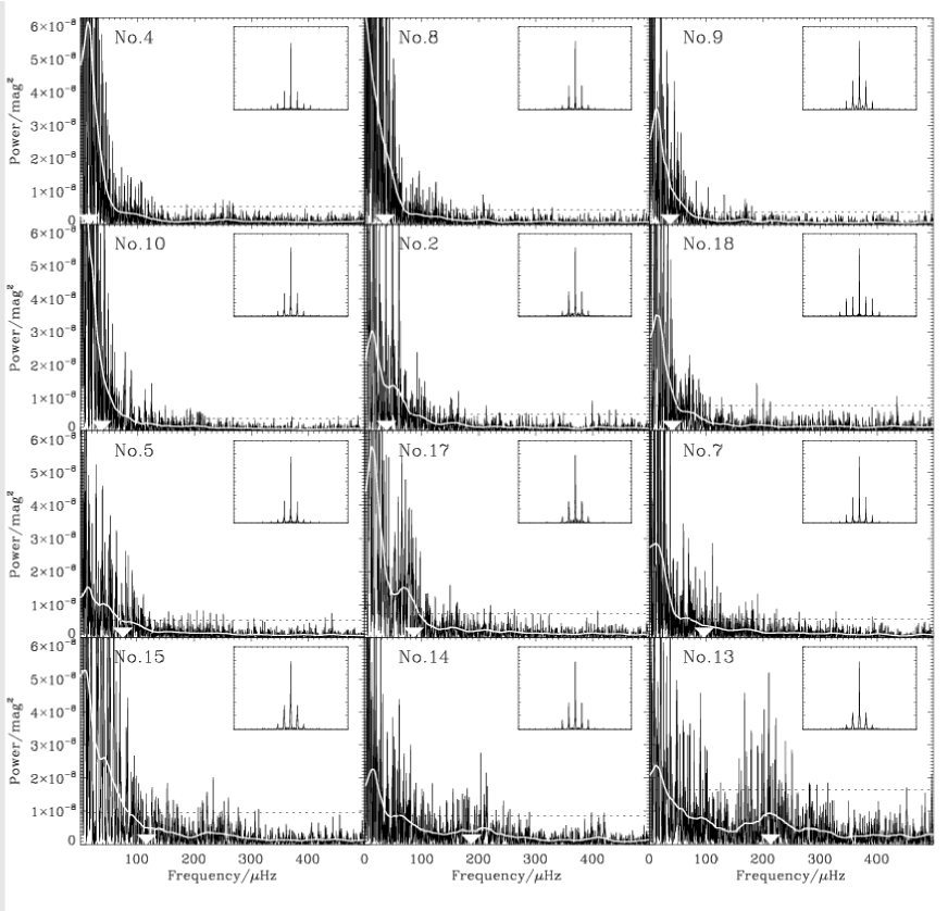
Figure 2: Fourier spectra of red giant stars (identifier shown in each panel). The solid white line is the smoothed spectrum, and the white arrow head indicates where we expect the stellar excess power (Table LABEL:tab2). The dotted horizontal line shows $(3\sigma_{300\mathrm{-}900\,\mu\mathrm{Hz}})^{2}$. The inset shows the spectral window on the same frequency scale as the main panel.

After the initial cleaning of the dominant low frequency noise peaks, we calculated the Fourier spectra of the combined data to search for excess power. The Fourier spectra were divided by the response function of the cleaning process to restore the overall power distribution. The response function was obtained by performing the same cleaning process on simulated time series of white noise with the same window function as the observations. The final response function for each star and each site was the average Fourier spectrum based on 100 simulations. In Fig. 2 we show the spectra of the best twelve stars (noise below 50$\,\mu$mag in the frequency range 300–900$\,\mu$Hz). Three other stars (Nos. 16, 19 and 20) fulfill this criterion but have been omitted due to significantly higher noise levels compared to stars of similar brightness. The solid white line in each panel of Fig. 2 is the smoothed spectrum, which was obtained by smoothing twice, with a boxcar width of 30$\,\mu$Hz followed by one of 10$\,\mu$Hz. The frequencies where we expect the stellar oscillations ($\nu_{\mathrm{max}}$, Eq. 2) are indicated with the white downward-pointing arrow head, and the dotted horizontal line shows $(3\sigma_{300\mathrm{-}900\,\mu\mathrm{Hz}})^{2}$. The increase in noise towards low frequencies, are due to drifts in the data from instrumental and atmospheric instabilities as discussed in Paper 1.

4.1 Location of excess power

We expect the oscillation modes to be located at lower frequencies for the more luminous stars (see Eq. 2 and Table LABEL:tab2). To search for general trends in the Fourier spectra, we grouped the stars according to luminosity. We formed three groups: the clump stars (5 stars), the stars between the clump and the lower RGB (4 stars), and the lower RGB stars (2 stars), but we excluded star No. 4 due to its sole location in the colour-magnitude diagram (see Fig. 1). For each group we averaged their Fourier spectra and smoothed the final spectrum. Smoothing was done twice. First, with a wide boxcar (width=100$\,\mu$Hz) to smear out humps of power originating from the individual spectra to better illustrate the overall distribution of power within each group. We then used a second boxcar (width=10$\,\mu$Hz) to smooth small point-to-point variations in the final plot. The result, shown in Fig. 3, confirms the general trend of shifting power excess as a function of luminosity, in agreement with expectations (see arrows in Fig. 3 showing expected location of excess power).

Figure 3: Average power distribution as a function of frequency for three groups of stars. The arrows show the mean position of the expected excess power, $\langle\nu_{\mathrm{max}}\rangle$, for the stars (stellar IDs in brackets) that have been used to calculate the corresponding power distribution (see text for details).

We investigated whether the observed power shift could have been produced by the reduction methods. (i) We inspected Fourier spectra and weights from each site and concluded that the power shift was not an artifact originating from high weights given to a few sites. (ii) We reanalysed the data without removing the peaks at 11.57, 23.15, 34.72 and 46.30$\,\mu$Hz, but saw the same trend, although with more power at low frequencies. (iii) Finally, we investigated whether our data reduction could introduce such a trend due to more pronounced drift noise for brighter and cooler stars. The best comparison stars for this purpose were the blue stragglers, which had similar brightness to the red giants and hence similar input parameters for the extraction of the photometry (for details see Kjeldsen & Frandsen, 1992,  and Paper I). However, their colours were very different from the red giants and from star to star, and only a few blue stragglers were observed at most sites. The blue stragglers showed different levels of excess power at low frequencies from star to star, but no causal relation could be found.

In summary, we found no evidence for a non-stellar source that could explain the observed pattern of excess power. The observed behaviour is exactly as expected for oscillations. However, due to the lack of a good ensemble of reference stars, similar to the red giant sample, we could not exclude with certainty that the photometric data reduction might have caused the shift as a result of more drift noise for more luminous and cooler stars.

4.2 Amplitude of excess power

To search for further evidence of solar-like oscillations, we measured the amount of excess power above the background noise, and converted that into amplitude per mode in order to compare it with expected amplitudes.

The noise level in the power spectrum, as a function of frequency, $p(\nu)$, was estimated using the following expression: $p(\nu)=a/\nu^{1.5}+p_{\mathrm{wn}}$. We tried $\nu$ to the power of $-1$, $-1.5$ and $-2$, and found $-1.5$ provided the best fit in the region around the excess power. We measured the white noise, $p_{\mathrm{wn}}$, as the mean level in the frequency range 300–900$\,\mu$Hz. Then, having fixed $p_{\mathrm{wn}}$, we calculated $a$ requiring that the integral of $p(\nu)$ in the range 50–900$\,\mu$Hz should equal that of the power spectrum. Assuming the excess power above this noise fit is real, we estimated the amplitude per mode based on the approach of Kjeldsen et al. (2005). These amplitude estimates are independent of the mode lifetime, but require an assumption of the number of modes that are excited. We have estimated the amplitudes for two extreme scenarios: (1) only radial modes are excited and, (2) three additional non-radial modes per radial mode, neglecting any difference in mode visibilities due to varying cancellations in full-disk observations. The approach is illustrated in Fig. 4 for three stars that all show a hump of power close to the expected frequency for solar-like oscillations (see arrow in left panels). The power spectra (Fig. 2) were divided by the integrated power of the spectral window to obtain power density spectra (Fig. 4 left panels). The background noise was subtracted from the smoothed spectra and the resulting power density was multiplied by the mean mode spacing ($\Delta\nu_{0}$ for only radial modes, and $\Delta\nu_{0}/4$ for both radial and non-radial modes). We then took the square root to convert to amplitude (Fig. 4 right panels).

The amplitude at $\nu_{\mathrm{max}}$ for each star is plotted versus $L/(MT_{\mathrm{eff}}^{2})$ in Fig. 5 and compared with results from simulations which used input amplitudes derived from Eq. 1. The filled dots corresponds to the values read from the solid black curves in Fig. 4 (right panels), while the empty circles in Fig. 5 corresponds to the solid grey curves (Fig. 4). However, for stars expected to oscillate at frequencies lower than $\sim 50\,\mu$Hz, we could not make realistic estimates of the noise contribution due to the apparent rapid rise in noise at low frequency, making it impossible to disentangle noise and stellar signal. We could only obtain upper limits, which are indicated with arrows in Fig. 5. Since these are upper limits, we only show the value derived assuming only radial modes are excited in these stars.

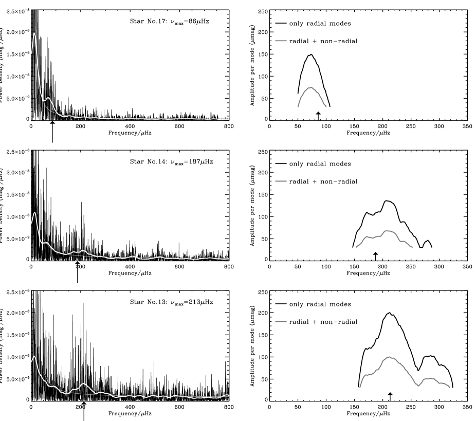
Figure 4: Left panels: Power density spectra of three selected red giant stars. The thick white solid line is the smoothed spectrum and the thin grey line is a fit to the noise. The arrow indicates the expected value of $\nu_{\mathrm{max}}$. Power density was calculated from Fig. 2 by dividing with the integrated power of the spectral window. Right panels: Estimated amplitudes for each of the three stars, derived by subtracting the noise from the smoothed power density spectrum, multiplying with $\Delta\nu_{0}/n$ ($n=1$ for radial modes only, $n=4$ for radial plus non-radial modes) and taking the square root.

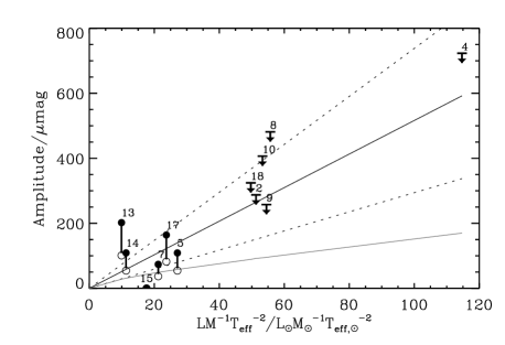
Figure 5: Measured amplitude versus $L/(MT_{\mathrm{eff}}^{2})$ for the best target stars (stellar IDs are indicated). Arrows show observed upper limits for stars where we could not estimate the noise contribution. For the other stars the filled dots (assuming only radial modes) and empty circles (assuming additional three non-radial modes) bracket the inferred amplitudes. The solid black line shows the mean amplitude from 100 simulations using Eq. 1 as input amplitude. The dotted lines are $\pm 2\sigma$, where $\sigma$ is the rms scatter in the simulations. The grey line indicates the mean amplitude based on $(L/M)^{0.7}$-scaling

Calculations by Christensen-Dalsgaard (2004) and Dziembowski et al. (2001) on more massive and luminous stars than our targets suggest that only radial modes are excited to observable amplitudes in red giant stars. No similar theoretical pulsation analysis have been published for the red giants in M67 in order to determine whether non-radial modes are expected. However, stars Nos. 13 and 14 are expected to oscillate at frequencies that are significantly higher than for typical red giant stars, and are similar to those of subgiants. Observations of the subgiants $\eta\,$Boo (Kjeldsen et al., 2003), $\beta\,$Hyi (Bedding et al., 2007) and $\nu\,$Ind (Carrier et al., 2007) clearly show evidence of both radial and non-radial modes.

The results in Fig. 5 show that most stars are in agreement with the scaling relation in Eq. 1 (illustrated with the black line). There is a tendency that the scaling based on $(L/M)^{0.7}$ (grey line) is in less good agreement with the data. However, we are not able to exclude either due to the uncertainty whether non-radial modes are present, and further because we only have upper limits for the most luminous stars. We note that for star No. 14 some non-radial modes are required to make the measured power excess in agreement (within $2\sigma$) with the scaling relation in Eq. 1. We further note that star No. 13 fall above the $2\sigma$ region even in the extreme case of three additional non-radial modes per radial mode. Hence, if the observed hump of power for this star is due to stellar oscillations, it is likely that non-radial modes are excited, and that we observed the star in a rare state of high amplitudes. The reason for this high excess power could also be due to more complicated drift noise in the data than described by our noise fit.

In summary, we see good evidence for oscillation power in three out of six stars that are expected to oscillate with frequencies larger than $50\,\mu$Hz. For stars expected to oscillated below $50\,\mu$Hz, we were only able to provided upper limits due to difficulties in determining the noise levels in their power spectra. In general we see agreement with the predicted amplitudes from $L/M$-scaling.

4.3 Autocorrelation of excess power

To search for a regular series of peaks, which is a typical signature of solar-like oscillations, we calculated the autocorrelation of all the stars in the frequency range where we expect stellar oscillations. For most stars the autocorrelation is dominated by the aliases at 1c/d. In about half the stars there is a hint of a peak that coincides with the expected large frequency separation (Eq. 3) and of those, there are two (Nos. 7 and 13) that show intriguing results. In the former, the most prominent peak is located at 8.8$\,\mu$Hz, which is very close to the expected value (Table LABEL:tab2). In Fig. 6 we show the autocorrelation of star No. 13. The autocorrelation was calculated in the frequency range 135–285$\,\mu$Hz setting all values in the Fourier spectrum lower than a threshold of $2\sigma_{300\mathrm{-}900\,\mu\mathrm{Hz}}$ (in amplitude) equal to the threshold value.

Figure 6: Autocorrelation of star No. 13 (see text). Dashed lines indicate integer multiples of one cycle per day (11.574$\,\mu$Hz).

The most significant peak that is not a daily alias is located at 19.3$\,\mu$Hz, which is within 15% of the expected value (Table LABEL:tab2).

4.4 Stellar granulation

In order to estimate the signal from background granulation we use a simple scaling of the solar granulation background observed by SoHO (VIRGO green channel). The scaling uses the Harvey model (Harvey, 1985) to describe the size and shape of the granulation power spectrum. The Harvey model needs as input the characteristic time scale for granulation, as well as the granulation scatter in the time series. We calibrated those two parameters using the solar data, using the following simple assumptions:

(1) The size of a granulation cell on the surface of a star is proportional to the scale height of the atmosphere at the stellar surface. The variance of the granulation in the time series is then assumed to be inverse proportional to the total number of cells on the surface.

(2) The characteristic time scale of granulation is approximated to be proportional to the ratio between the size of the individual cells and the velocity of the cell. We estimate the granulation cell velocities to be proportional to the sound speed in the stellar atmosphere.

(3) We assume that the atmosphere is isothermal (allowing a simple scaling of the atmospheric scale height).

More details can be found in Kjeldsen & Bedding (in preparation). Using these assumptions, we are able to calculate granulation power spectra that agrees both in shape and level with detailed simulations by Svensson & Ludwig (2004). In Fig. 7 we plot smoothed power density spectra of the target stars, together with the estimated signal from background granulation. For the most luminous stars granulation is likely to contribute significantly at low frequencies, while for the most faint stars in our sample granulation can be excluded as a possible cause of increasing noise. From this figure we can also see that there is a distinct difference in time scale between the granulation and the humps of power that appear to be due to stellar oscillations. Background granulation will therefore not prevent detection of solar-like oscillations.

Figure 7: Smoothed power density spectra of red giant stars (identifier shown in each panel). The dashed curve is the estimated granulation signal based on scaling from the Sun (see Sect 4.4). The dotted line indicates where stellar oscillations are expected (Eq. 2).

5 Simulations

Figure 8: Autocorrelation of a simulation of star No. 13 (see text). Dashed lines indicate integer multiples of one cycle per day (11.574$\,\mu$Hz).

To interpret the results shown in Sect. 4, we made a series of simulations of each target star using the method described by Stello et al. (2004). We chose a regular series of input frequencies with a separation of $\Delta\nu_{0}$ (Table LABEL:tab2). Their relative amplitudes were determined by a Gaussian envelope with a height corresponding to the $L/M$-scaling values in Table LABEL:tab2 (note that $(L/M)^{0.7}$-scaling predicts amplitudes that are roughly 0.3–0.5 times that for our targets). The envelope was centered at $\nu_{\mathrm{max}}$ (Table LABEL:tab2) with a width equal to $0.48\,\nu_{\mathrm{max}}$, which was calibrated to the observations of $\xi\,$Hya (Stello et al., 2004). The envelope reproduced by this approach is in good agreement with $\beta\,$Hyi and the Sun (Kjeldsen et al., 2005). The number of input frequencies was the closest integer of $7\times 0.48\,\nu_{\mathrm{max}}/\Delta\nu_{0}$, which ensures that we have frequencies within the entire envelope. Because the non-white noise is difficult to estimate precisely, we chose to include only white noise in the simulations, which we set equal to the mean level in the Fourier spectra at 300–900$\,\mu$Hz of the observed data. For each target star we ran simulations in two parallel runs, one with a mode lifetime of 20 days, in agreement with the theoretical calculations on the red giant $\xi\,$Hya (Houdek & Gough, 2002), and the other of 2 days in agreements with the observations of that star (Stello et al., 2006).

We show here the results for the short mode lifetime (Fig. 9). The difference between the long and short mode lifetime is discussed below. It is important to stress that the detailed characteristics of the excess power in the Fourier spectra depend very much on the complicated interaction between the spectral window and the oscillation modes (their frequencies, amplitudes and lifetime), as well as the random number seed. For example, using the same random number seed, the clump stars (Nos. 8, 9, 10, 2 and 18), which had different spectral windows but only slightly different amplitudes and input frequencies, show very different power excesses (Fig. 9). For star No. 2 we show in Fig. 10 (left panels) five spectra based on different random number seeds. Again, we see a large variation in the result, which is in agreement with Fig. 5 (dashed lines). This large intrinsic variation was also pointed out by Stello et al. (2004, 2006). The right panels show the corresponding spectra based on the long mode lifetime (=$20\,$days). From this, we see that a long mode lifetime in general provides higher peaks, but the differences are comparable to the difference that arises from using a different seed.

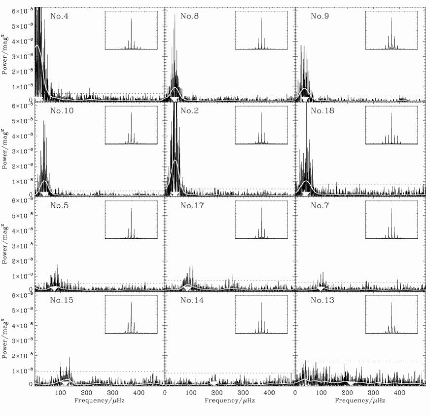
Figure 9: Fourier spectra of simulated red giant stars (identifier shown in each panel), with a mode lifetime of 2 days and amplitudes according to $L/M$-scaling (Eq. 1). The solid white line is the smoothed spectrum, and the white arrow head indicates where we expect the stellar excess power (Table LABEL:tab2). The inset shows the spectral window on the same frequency scale as the main panel. The dotted line is $(3\sigma_{300\mathrm{-}900\,\mu\mathrm{Hz}})^{2}$.

A comparison of observations and simulations (Figs. 2 and 9) indicates that a significant part of the excess power seen in the observations might be of stellar origin. The excess power in the observations can be associated with either humps of power (see Nos. 13 and 17 in Fig. 2) or a broad “shoulder” on top of the drift noise (see No. 2). It is clear from the simulations that observing excess power in one star does not imply that we necessarily would see a similar hump in a similar star (or even in the same star if observed at another epoch; Fig. 10). We note that the simulations shown in Fig. 9 only included radial modes. If the stars have non-radial modes these simulations underestimate the stellar excess power. This could be significant at least for the less evolved stars (Nos. 13 and 14). Very recently, Hekker et al. (2006) reported that non-radial modes are present in two red giant stars ($\varepsilon\,$Oph and $\eta\,$Ser) that oscillate at approximately $60\,\mu$Hz and $130\,\mu$Hz, respectively, and hence are comparable to stars in our sample. Here we also note that the scaling relation that was used to estimate the amplitudes is quite uncertain for red giant stars.

Finally, we calculated the autocorrelation of simulated data of star No. 13 that reproduced the observed excess power. This was done by setting the input amplitude of the simulations to $200\,\mu$mag and including only radial modes in accordance with Fig. 4. This time we set the white noise equal to the value estimated at 200$\,\mu$Hz from our noise fit in Fig. 4. The autocorrelation was based on simulations with a short mode lifetime (= 2 days) because they produced Fourier spectra more like the observed spectrum. In total nine independent simulations were made. In roughly half the cases we saw a peak in the autocorrelation of the same significance as in the observations (Fig. 6). In Fig. 8 we show one of the examples which show a peak. However, these peaks were not at exactly the same frequency but appeared in an interval from approximately 16$\,\mu$Hz to 19$\,\mu$Hz. Some of these (as in Fig. 8) were close to halfway between 1 and 2 cycles per day (17.4$\,\mu$Hz), and might therefore be caused by aliasing. In the other cases the only clear peaks were those clearly originating from the daily aliases at 1, 2 and 3 cycles per day.

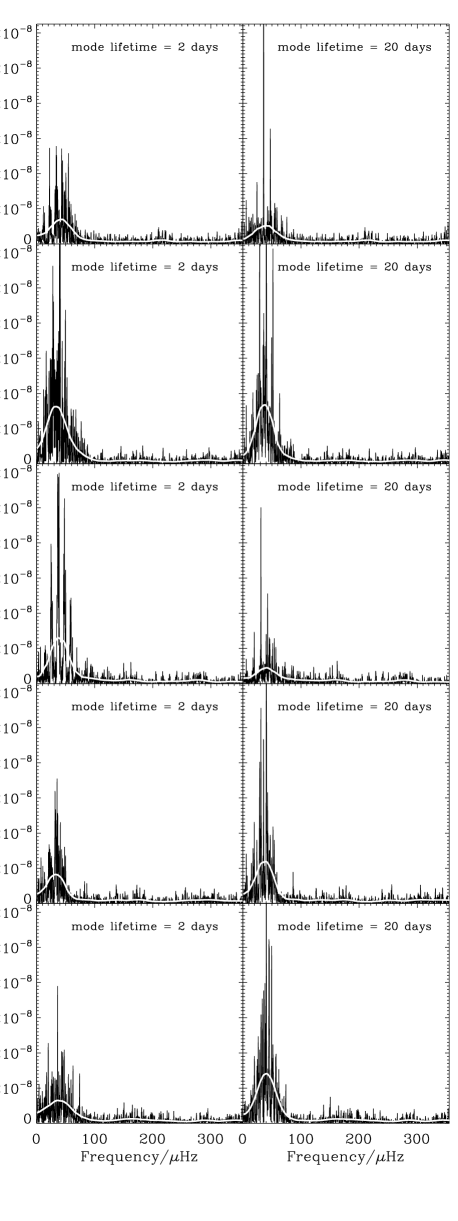
Figure 10: Fourier spectra of simulated data (star No. 2) for five different random number seeds and two different mode lifetimes (left: 2 days, right: 20 days). The solid white line is the smoothed spectrum.

To investigate whether the peak seen at 19.3$\,\mu$Hz in the autocorrelation of the observations was caused by interaction between the spectral window and random peaks we repeated the simulations using randomly spaced frequencies. For each of the three sets of random frequencies we made nine independent simulations, and inspected the autocorrelation. The differences seen between each of the independent simulations within each set of frequencies were small compared to the difference between different sets. In most cases we did not see a clear peak in the range 16–19$\,\mu$Hz, but in a few cases a clear peak halfway between 1 and 2 cycles per day (17.4$\,\mu$Hz) was seen. In some cases peaks as significant as the observed 19.3$\,\mu$Hz peak were seen at other frequencies. Hence, we conclude that the peak at 19.3$\,\mu$Hz in the observations could be caused by randomly distributed peaks.

6 Conclusions

We have analysed high-precision photometric time series of 20 red giant stars in the open cluster M67. The data, recently published in Paper I, were from a large multisite campaign.

We see evidence of excess power in the Fourier spectra, shifting to lower frequencies for more luminous stars, consistent with expectations from solar-like oscillations (see Fig. 3).

We further estimated the mode amplitude from the observed power excess assuming that it originates from solar-like oscillations. These estimated amplitudes are in agreement with the results from simulations using estimated amplitudes by scaling from the Sun (Fig. 5). These results further support that we have seen evidence for solar-like oscillations in some of the red giant stars in M67. We note that the measured amplitudes from our simulations show a scatter of roughly 40% from one epoch to the next, which is similar to what we see in the Sun (Kjeldsen et al., 2007). This intrinsic scatter should always be taken into account when evaluating observed amplitudes of solar-like oscillations. Without firm knowledge of whether non-radial modes are present in these stars and with only upper limits on the amplitudes of the most luminous stars, the large scatter in the measured amplitude limits our ability to clearly pinpoint a favoured scaling relation for amplitude. However, we see an indication of a better match between observations and the $L/M$-scaling (Kjeldsen & Bedding, 1995) than with $(L/M)^{0.7}$-scaling (Samadi et al., 2005).

In many stars we see apparently high levels of non-white noise, but its temporal variation is unknown and could not be decorrelated. In the Fourier spectrum this noise seems to be significant at frequencies below 100$\,\mu$Hz. This is unfortunate because the target stars in which we expected the most clear detections are expected to be oscillating in the affected frequency range. We are therefore not able to disentangle the noise and stellar signal in the analysis of these stars. Hence, the data did not allow the clear detections that we had anticipated. Simple scaling of the solar granulation (Harvey, 1985) shows that the power at low frequencies (lower than the expected p-mode range) is not coming from granulation for the fainter stars on the low RGB, and is most likely instrumental (see Fig. 7). However, it could be granulation noise in the more luminous clump stars and star No. 4 (see Fig. 1).

If the observed power excesses are due to stellar oscillations this result shows great prospects for asteroseismology on clusters. However, with the unfortunate cancellation of the Eddington mission by ESA, we might have to wait many years for a dedicated space project specifically aiming at asteroseismology on stellar clusters. Alternatively, one could initiate a ground-based network with high-resolution and high-sensitivity spectrographs that is able to detect oscillations in faint cluster stars, or a photometric multisite campaign with larger telescopes (preferably larger than 2 meter, see Paper I) with stable instrumentation located at good sites aimed at red giants in clusters. As clearly demonstrated by our results, the final level of the non-white noise (including drift) in the data will be absolutely crucial in any approach to detect solar-like oscillations in red giant stars. This largely favours space missions as atmospheric effects in ground-based data varies on time scales similar to the stellar oscillations. Although the Kepler and COROT space missions will not specifically target clusters it is expected that these missions will observe many red giants, some of which would be in clusters. Recent results from the MOST satellite on the red giant $\varepsilon\,$Oph (Barban et al., 2007) demonstrates that space missions have the potential to do very interesting science on red giant field stars, and more K giants are on the target list for MOST in the future.

We would be happy to make the data presented in this paper available on request.

References

- Allen (1973) Allen C. W., 1973, Astrophysical quantities. London: University of London, Athlone Press, —c1973, 3rd ed.
- Barban et al. (2004) Barban C., De Ridder J., Mazumdar A., Carrier F., Eggenberger P., de Ruyter S., Vanautgaerden J., Bouchy F., Aerts C., 2004, in Proceedings of the SOHO 14 / GONG 2004 Workshop (ESA SP-559). ”Helio- and Asteroseismology: Towards a Golden Future”. 12-16 July, 2004. New Haven, Connecticut, USA. Editor: D. Danesy., p.113 Detection of Solar-Like Oscillations in Two Red Giant Stars. p. 113
- Barban et al. (2007) Barban C., Matthews J. M., De Ridder J., Baudin F., Kuschnig R., Mazumdar A., Samadi R., Guenther D. B., Moffat A. F. J., Rucinski S. M., Sasselov D., Walker G. A. H., Weiss W. W., 2007, Detection of solar-like oscillations in the red giant star eps Oph by MOST spacebased photometry, submitted to A&A
- Bedding & Kjeldsen (2003) Bedding T. R., Kjeldsen H., 2003, Publications of the Astronomical Society of Australia, 20, 203
- Bedding et al. (2007) Bedding T. R., Kjeldsen H., Arentoft T., O’Toole S. J., 2007, Solar-like oscillations in the G2 subgiant Hydri from dual-site observations, submitted to ApJ
- Brown et al. (1991) Brown T. M., Gilliland R. L., Noyes R. W., Ramsey L. W., 1991, ApJ, 368, 599
- Carrier et al. (2007) Carrier F., Kjeldsen H., Bedding T. R., Brewer B. J., Butler R. P., Eggenberger P., Grundahl F., McCarthy C., Retter A., Tinney C. G., 2007, Solar-like oscillations in the metal-poor subgiant Indi: acoustic spectrum and mode lifetime, submitted to A&A
- Christensen-Dalsgaard (2004) Christensen-Dalsgaard J., 2004, Sol. Phys., 220, 137
- De Ridder et al. (2006) De Ridder J., Barban C., Carrier F., Mazumdar A., Eggenberger P., Aerts C., Deruyter S., Vanautgaerden J., 2006, A&A, 448, 689
- Dziembowski et al. (2001) Dziembowski W. A., Gough D. O., Houdek G., Sienkiewicz R., 2001, MNRAS, 328, 601
- Frandsen et al. (2002) Frandsen S., Carrier F., Aerts C., Stello D., Maas T., Burnet M., Bruntt H., Teixeira T. C., de Medeiros J. R., Bouchy F., Kjeldsen H., Pijpers F., Christensen-Dalsgaard J., 2002, A&A, 394, L5
- Gilliland & Brown (1988) Gilliland R. L., Brown T. M., 1988, PASP, 100, 754
- Gilliland & Brown (1992) Gilliland R. L., Brown T. M., 1992, PASP, 104, 582
- Gilliland et al. (1991) Gilliland R. L., Brown T. M., Duncan D. K., Suntzeff N. B., Lockwood G. W., Thompson D. T., Schild R. E., Jeffrey W. A., Penprase B. E., 1991, AJ, 101, 541
- Gilliland et al. (1993) Gilliland R. L., Brown T. M., Kjeldsen H., McCarthy J. K., Peri M. L., Belmonte J. A., Vidal I., Cram L. E., Palmer J., Frandsen S., Parthasarathy M., Petro L., Schneider H., Stetson P. B., Weiss W. W., 1993, AJ, 106, 2441
- Girard et al. (1989) Girard T. M., Grundy W. M., Lopez C. E., van Altena W. F., 1989, AJ, 98, 227
- Harvey (1985) Harvey J., 1985, in Rolfe E., Battrick B., eds, ESA SP-235: Future Missions in Solar, Heliospheric & Space Plasma Physics High-Resolution Helioseismology. p. 199
- Hekker et al. (2006) Hekker S., Aerts C., de Ridder J., Carrier F., 2006, A&A, 458, 931
- Honeycutt (1992) Honeycutt R. K., 1992, PASP, 104, 435
- Houdek & Gough (2002) Houdek G., Gough D. O., 2002, MNRAS, 336, L65
- Kjeldsen & Bedding (1995) Kjeldsen H., Bedding T. R., 1995, A&A, 293, 87
- Kjeldsen et al. (2007) Kjeldsen H., Bedding T. R., Arentoft T., Butler R. P., Bouchy F., Dall T. H., Karoff C., Kiss L. L., Tinney C. G., 2007, The amplitude of solar oscillations using stellar techniques, submitted to ApJ
- Kjeldsen et al. (2003) Kjeldsen H., Bedding T. R., Baldry I. K., Bruntt H., Butler R. P., Fischer D. A., Frandsen S., Gates E. L., Grundahl F., Lang K., Marcy G. W., Misch A., Vogt S. S., 2003, AJ, 126, 1483
- Kjeldsen et al. (2005) Kjeldsen H., Bedding T. R., Butler R. P., Christensen-Dalsgaard J., Kiss L. L., McCarthy C., Marcy G. W., Tinney C. G., Wright J. T., 2005, ApJ, 635, 1281
- Kjeldsen & Frandsen (1992) Kjeldsen H., Frandsen S., 1992, PASP, 104, 413
- Lejeune et al. (1998) Lejeune T., Cuisinier F., Buser R., 1998, A&AS, 130, 65
- Montgomery et al. (1993) Montgomery K. A., Marschall L. A., Janes K. A., 1993, AJ, 106, 181
- Nissen et al. (1987) Nissen P. E., Twarog B. A., Crawford D. L., 1987, AJ, 93, 634
- Pietrinferni et al. (2004) Pietrinferni A., Cassisi S., Salaris M., Castelli F., 2004, ApJ, 612, 168
- Samadi et al. (2005) Samadi R., Goupil M.-J., Alecian E., Baudin F., Georgobiani D., Trampedach R., Stein R., Nordlund Å., 2005, JApA, 26, 171
- Sanders (1977) Sanders W. L., 1977, A&AS, 27, 89
- Stello (2002) Stello D., 2002, Master’s thesis, Institut for Fysik og Astronomi, Aarhus Universitet
- Stello et al. (2006) Stello D., Arentoft T., Bedding T. R., Bouzid M. Y., Bruntt H., Csubry Z., Dall T. H., Dind Z. E., Frandsen S., Gilliland R. L., Jacob A. P., Jensen H. R., Kang Y. B., Kim S.-L., Kiss L. L., Kjeldsen H., Koo J.-R., Lee J.-A., Lee C.-U., Nuspl J., Sterken C., 2006, MNRAS, 373, 1141
- Stello et al. (2006) Stello D., Kjeldsen H., Bedding T. R., Buzasi D., 2006, A&A, 448, 709
- Stello et al. (2004) Stello D., Kjeldsen H., Bedding T. R., De Ridder J., Aerts C., Carrier F., Frandsen S., 2004, Sol. Phys., 220, 207
- Svensson & Ludwig (2004) Svensson F., Ludwig H. ., 2004, ArXiv Astrophysics e-prints
- Teixeira et al. (2003) Teixeira T. C., Christensen-Dalsgaard J., Carrier F., Aerts C., Frandsen S., Stello D., Maas T., Burnet M., Bruntt H., de Medeiros J. R., Bouchy F., Kjeldsen H., Pijpers F., 2003, Ap&SS, 284, 233
- VandenBerg & Stetson (2004) VandenBerg D. A., Stetson P. B., 2004, PASP, 116, 997
- Zhao et al. (1993) Zhao J. L., Tian K. P., Pan R. S., He Y. P., Shi H. M., 1993, A&AS, 100, 243