Evaluating Spectral Models and the X-ray States of Neutron-Star X-ray Transients

Abstract

We analyze the X-ray spectra of the neutron-star (NS) X-ray transients Aql X-1 (catalog ) and 4U 1608-52 (catalog ), obtained with RXTE during more than twenty outbursts. Our aim is to properly decompose the spectral components and to study their evolution across the hard and soft X-ray states. We test commonly used spectral models and evaluate their performance against desirability criteria, including $L_{\rm X}\propto T^{4}$ evolution for the multicolor disk (MCD) component, and similarity to black holes (BHs) for correlated timing/spectral behavior. None of the classical models for thermal emission plus Comptonization perform well in the soft state. Instead, we devise a hybrid model: for the hard state a single-temperature blackbody (BB) plus a broken power-law (BPL) and for the soft state two thermal components (MCD and BB) plus a constrained BPL. This model produces $L_{\rm X}\propto T^{4}$ tracks for both the MCD and BB, and it aligns the spectral/timing correlations of these NSs with the properties of accreting BHs. The visible BB emission area is very small ($\sim$ $1/16$ of the NS surface), but it remains roughly constant over a wide range of $L_{\rm X}$ that spans both the hard and soft states. We discuss implications of a small and constant boundary layer in terms of the presence of an innermost stable circular orbit that lies outside the NS. Finally, if the BB luminosity tracks the overall accretion rate, then we find that the Comptonization in the hard state has surprisingly high radiative efficiency, compared to MCD emission in the soft state. Alternatively, if we assume that the radiative efficiency of a jet in the hard state must be less than the MCD efficiency in the soft state, while relaxing presumptions about the accretion rate, then our results may suggest substantial mass outflow in the jet.

1. INTRODUCTION

In low-mass X-ray binaries (LMXBs), a neutron star (NS) or stellar-mass black hole (BH) accretes matter from a Roche-lobe filling, low-mass companion star through an accretion disk. X-rays are produced by the inner accretion disk and/or the boundary layer formed by impact of the accretion flow with the NS surface. The luminous and weakly magnetized NS LMXBs are classified into atoll and Z sources based on their X-ray spectral and timing properties (Hasinger & van der Klis, 1989). In a color-color diagram, Z sources trace out roughly Z-shaped tracks within hours to a day or so. Their X-ray spectra are normally soft in all three branches of the “Z”, i.e., most of the flux is emitted below 20 keV. Atoll sources, however, show more dramatic spectral changes, albeit on longer time scales (days to weeks); their spectra are usually soft at high luminosities and hard when they are faint.

Recently, it was found that some atoll sources can also exhibit Z-shaped tracks in the color-color diagram when they are observed over a large range of luminosity (Muno et al., 2002; Gierliński & Done, 2002a). However, it was noted by several authors (Barret & Olive, 2002; van Straaten et al., 2003; Reig et al., 2004; van der Klis, 2006) that the properties of atoll sources (e.g., rapid X-ray variability, the order in which branches are traced out) are very different from those of the Z sources. The spectral states of atoll sources in the upper, diagonal and lower branches of these Z-shaped tracks are often referred to as the “extreme island”, “island”, and “banana” states/branches, respectively. However, in this paper we will use the terms “hard”, “transitional”, and “soft” states, respectively.

The spectral modeling of accreting NSs has been controversial for a long time (see Barret, 2001, for a review). In the soft state, the spectra are generally described by models that include a soft/thermal and a hard/Comptonized component. Based on the choice of the thermal and Comptonized components, there are two classical models, often referred to as the Eastern model (after Mitsuda et al., 1989) and the Western model (after White et al., 1988). In the Eastern model, the thermal and Comptonized components are described by a multicolor disk blackbody (MCD) and a weakly Comptonized blackbody, respectively. In the Western model, the thermal component is a single-temperature blackbody (BB) from the boundary layer and there is Comptonized emission from the disk. The color temperature for the thermal component (i.e., the temperature at the inner disk radius $kT_{\rm mcd}$ for a disk model or $kT_{\rm bb}$ for a boundary layer model) is typically in the range of $\sim$ 0.5–2.0 keV (e.g., Barret et al., 2000; Oosterbroek et al., 2001; Di Salvo et al., 2000a; Iaria et al., 2005). For the Comptonized component, the same authors reported a plasma temperature of $\sim$ 2–3 keV and a large optical depth of $\sim$ 5–15 in the soft state (for a spherical geometry).

In the hard state, the spectra are dominated by a hard/Comptonized component, but a soft/thermal component is generally still required (Christian & Swank, 1997; Barret et al., 2000; Church & Balucińska-Church, 2001; Gierliński & Done, 2002b). The thermal component can be either a BB or a MCD, but the latter seems to be ruled out by the inferred inner disk radii that are unphysically small. The color temperature of this component is typically $\lesssim$ 1 keV (e.g., Barret et al., 2003; Church & Balucińska-Church, 2001). The inferred plasma electron temperature of the Comptonized component is typically a few tens of keV and its optical depth is $\sim$ 2–3 in the hard state (for a spherical geometry). The hard state of atoll sources is considered by some authors to be associated with a steady jet (e.g., Fender, 2006; Migliari & Fender, 2006). The inverse Compton spectrum could then arise from the base of the jet, and synchrotron emission would contribute seed photons and perhaps a secondary contribution to the X-ray spectrum (Markoff et al., 2005).

In the past, various approaches have been made to further our understanding of X-ray spectra of accreting NSs. These include: (1) spectral surveys of a large number of sources, covering a wide range of luminosities (Church & Balucińska-Church, 2001; Christian & Swank, 1997), (2) detailed studies of a large number of observations from a single outburst of a NS X-ray transient (Gierliński & Done, 2002b; Maccarone & Coppi, 2003b; Maitra & Bailyn, 2004), (3) Fourier frequency resolved X-ray spectroscopy (Gilfanov et al., 2003; Olive et al., 2003), and (4) comparisons of spectral and timing properties to those of BH LMXBs, to understand which features might be the result of the presence/absence of a solid surface (Wijnands, 2001; Barret, 2001; Done & Gierliński, 2003). However, a general consensus on the appropriate X-ray spectral model for the various subtypes and states of accreting NSs has not been achieved.

In this paper we present an extensive study of a large number of observations of two NS transients Aql X-1 (catalog ) and 4U 1608-52 (catalog ), using data obtained with the Rossi X-ray Timing Explorer (RXTE , Bradt et al., 1993), during more than twenty individual outbursts. There are several advantages of using this archive. First, it allows us to compare the evolution of spectral properties of different outbursts systematically. Second, we can examine the behavior of a specific spectral component with changes in accretion rate, capitalizing on the large range in luminosity exhibited by these atoll-type transients. Third, compared with surveys using just a few observations but many sources, we can reduce the problems due to our poor knowledge of the parameters of the sources (e.g., the distance, inclination, and absorption).

The goal of this paper is to find a spectral model that can well describe the X-ray spectra of NS X-ray transients. Although the NS X-ray transients often change luminosity by several orders of magnitude and show substantial diversity in outbursts, their well organized color-color and color-intensity diagrams clearly show that their spectral evolution tracks are narrow and thus repeatable. This compels the efforts to unlock spectral models for NS systems to explain the well-behaved sources in terms of accretion physics, and also to further investigate the differences and similarities between BHs and NSs.

Aql X-1 (catalog ) and 4U 1608-52 (catalog ) have been classified as atoll sources (Hasinger & van der Klis, 1989; Reig et al., 2000). Recently, Reig et al. (2004) and van Straaten et al. (2003) analyzed the general timing properties of these two sources. Here we will concentrate on their spectral properties. We describe our data reduction scheme in §2 and show the long-term light curves and color-color diagrams in §3. We perform and evaluate detailed spectral modeling in §4. In §5, we compare timing properties with BHs in order to further evaluate the spectral models. We argue that a particular model is most suitable for these NS transients, and then we further explore the ramifications of this model for X-ray states and the physical properties of accretions in §6 and §7. Finally we give our summary and discussion.

2. OBSERVATIONS AND DATA REDUCTION

For our analysis, we used all of the available RXTE observations of Aql X-1 (catalog ) and 4U 1608-52 (catalog ) prior to 2006 January 1. Data were analyzed from the Proportional Counter Array (PCA; Jahoda et al., 1996) and the High Energy X-ray Timing Experiment (HEXTE; Rothschild et al., 1998) instruments. We utilized the best-calibrated detector units of each instrument, which are Proportional Counter Unit 2 (PCU 2) for the PCA and Cluster A for the HEXTE, and we extracted the average pulse-height spectra, one for each RXTE observation. All spectral extractions and analyses utilized the FTOOLS software package version 6.0.4. Some standard criteria were used to filter the data: data of 20 seconds before and 200 seconds after type I X-ray bursts were excluded (see Remillard et al., 2006); the earth-limb elevation angle was required to be larger than $10\arcdeg$; the spacecraft pointing offset was required to be $<0.02\arcdeg$. For faint observations, we additionally excluded data within 30 minutes of the peak of South Atlantic Anomaly passage or with large trapped electron contamination.

We only considered observations that yielded data from the PCA, HEXTE and relevant spacecraft telemetry. Only observations with PCA intensity (background subtracted) larger than 10 counts/s/PCU were used. We required the exposure of the spectra to be larger than five minutes for faint observations (source intensity lower than 40 counts/s/PCU) and two minutes for bright observations. Appropriate faint/bright background models were used when the source had intensity lower or higher than 40 counts$/$s$/$PCU. For the PCA, the spectra were extracted from “standard 2” data collection mode and the response files were created so that they were never offset from the time of each observation by more than 20 days. For the HEXTE, the program HXTLCURV was used for spectral extraction, background subtraction, and deadtime correction. Finally, we applied systematic errors of $0.8\%$ for PCA channel 0–39 (about below 18 keV) and $2\%$ for PCA channel 40–128 (Kreykenbohm et al., 2004; Jahoda et al., 2006). No systematic errors were applied for HEXTE data. A summary of the observations and other source properties is given in Table 1. All further analyses and spectral fits were uniformly applied to each selected observation.

3. LIGHT CURVES AND COLOR-COLOR DIAGRAMS

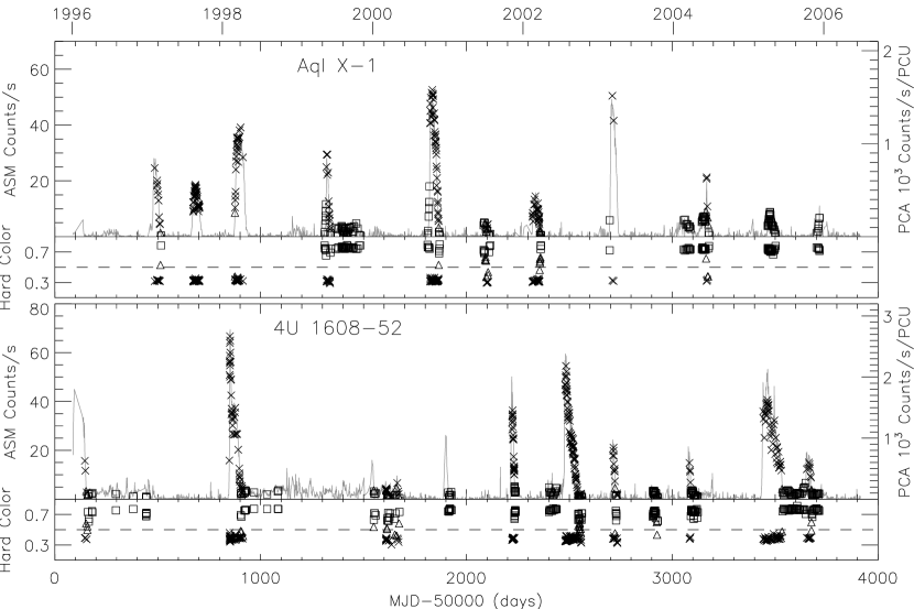
Figure 1.— Long-term light and color curves of Aql X–1 and 4U 1608–52, showing a large variety of outburst properties. Grey solid lines are from RXTE ASM and discrete symbols are from PCA observations representing different spectral states: hard (square), transitional (triangle), and soft (cross). The dashed line (hard color = 0.5) is a reference to help distinguish the different states.

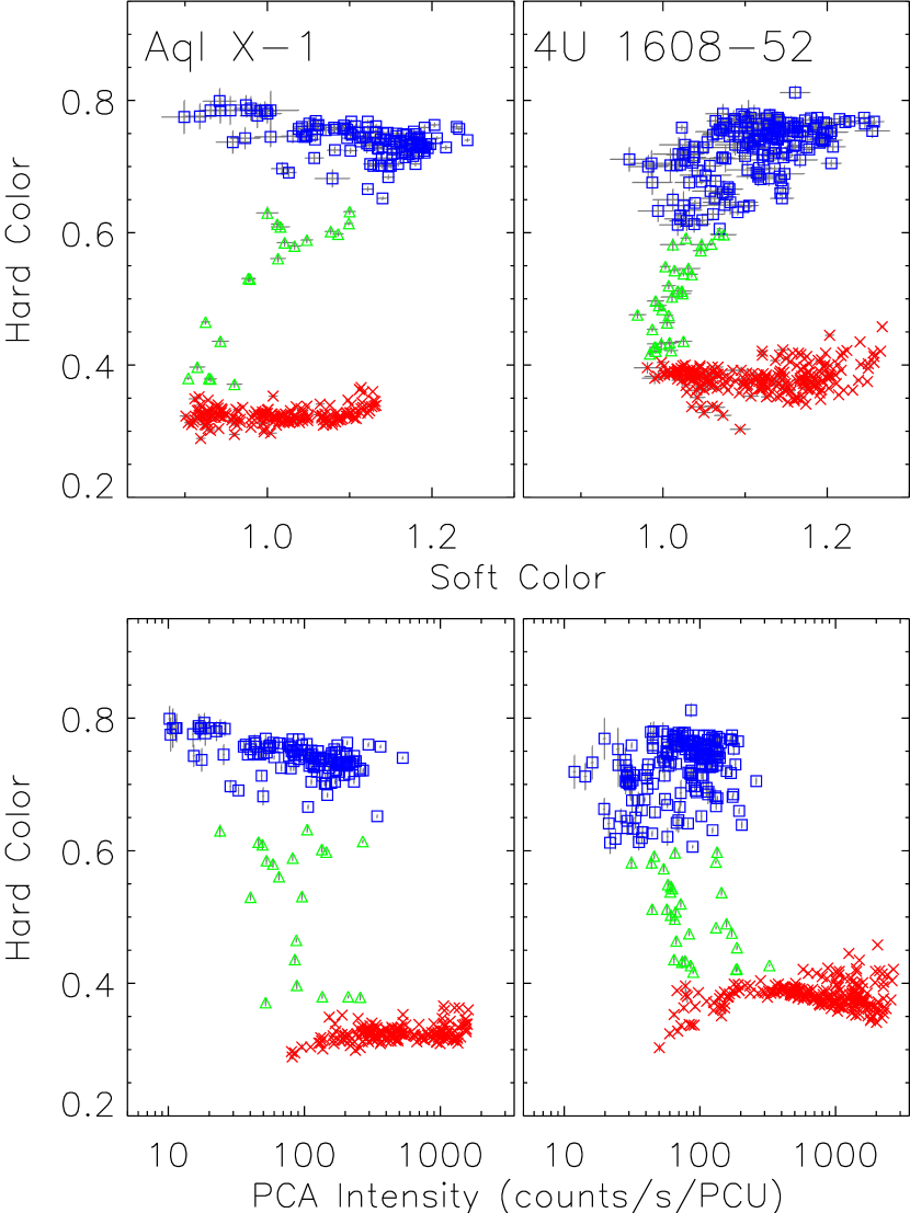
Figure 2.— Normalized color-color and color-intensity diagrams of Aql X–1 and 4U 1608–52 from ten years of pointed RXTE PCA observations. The PCA intensity is the normalized count rate from PCU2, and in these units the Crab Nebula yields 2520 c/s. The hard, transitional, and soft states are represented by blue squares, green triangles, and red crosses, respectively. The uncertainties are at 1 $\sigma$ confidence and are normally smaller than the symbol size.

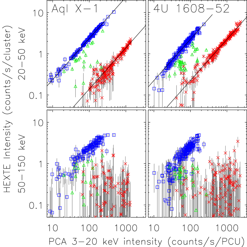
Figure 3.— The HEXTE intensity in two hard energy bands versus the PCA intensity at 3–20 keV. The solid lines show linear fits for these measurements. The hard and soft states appear increasingly different when they are compared using more widely spaced energy bands.

The long-term light and color curves of Aql X-1 (catalog ) and 4U 1608-52 (catalog ) are shown in Figure 1. This figure combines data from the PCA and the RXTE All-Sky Monitor (ASM; Levine et al., 1996). Typically, outbursts start in the hard state, evolve to the soft state, and finally return to the hard state during the decay. However, outbursts can be quite different from each other, e.g., in amplitude and duration. Moreover, in some outbursts the source did not enter the soft state.

For each observation we calculated X-ray colors, in a manner similar to Muno et al. (2002). Soft and hard colors were defined as the ratios of the background-subtracted counts in the (3.6–5.0)/(2.2–3.6) keV bands and the (8.6–18.0)/(5.0–8.6) keV bands, respectively. We normalized the raw count rates from each PCU with the help of observations of the Crab Nebula. For each PCA gain epoch, we computed linear fits (vs. time) to normalize the Crab count rates to target values of 550, 550, 850, and 570 counts/s/PCU in these four energy bands. The normalized color-color and color-intensity diagrams in Figure 2 resemble those in Muno et al. (2002), although our figure includes more data and we used a different normalization scheme for the softest energy bands. Although these two sources are atoll sources, their tracks in the color-color diagrams are Z-shaped, owing to their large range of luminosities. We combined the hard color and PCA intensity to pragmatically define the source states as shown in Figure 2. The hard state has a hard color $>0.65$ (Aql X-1 (catalog )) or $>0.6$ (4U 1608-52 (catalog )); the soft state has a PCA intensity $>400$ counts/s/PCU and a hard color $<0.5$ or a PCA intensity $<400$ counts/s/PCU and a hard color $<0.36$ (Aql X-1 (catalog )) or $<0.41$ (4U 1608-52 (catalog )). All of the remaining observations are referred to as the transitional state. For all figures in this paper, the hard, transitional, and soft states are represented by blue squares, green triangles, and red crosses, respectively. We note that strong hysteresis is observed in both sources, that is, the hard-soft transition generally occurs at higher X-ray flux compared to the soft-hard transition (e.g., Maccarone & Coppi, 2003a). The transitional-state observations are mostly from the decay phases of the outbursts, since the rise is often sparsely covered.

Figure 3 shows the relation of source intensities in more widely spaced energy bands. The top panels are the HEXTE 20–50 keV intensity versus the PCA 3–20 keV intensity. The most striking aspect of these panels is that there are two nearly linear tracks corresponding to the soft and hard states. The bottom panels are the HEXTE 50–150 keV intensity versus the PCA 3–20 keV intensity. We can still see the linear track in the hard state, but the sources are generally not detected above 50 keV in the soft state.

While the light curves in Figure 1 show substantial diversity in outburst amplitude and duration for a given source, Figures 2 and 3 show that the superposition of all observations on color-color and color-intensity diagrams shows well organized spectral states and very common behaviors in these two sources. The aim of this paper is to capitalize on this organization and the comprehensive RXTE data archive, in order to determine the best way to model the X-ray spectra across these different states.

4. SPECTRAL MODELING

4.1. Spectral Models and Assumptions

In this work, we fitted the X-ray spectra of Aql X-1 (catalog ) and 4U 1608-52 (catalog ) with several different models. The PCA and HEXTE pulse-height spectra were fitted jointly over the energy range 2.6–23.0 keV and 20.0–150.0 keV, respectively, allowing the normalization of the HEXTE spectrum, relative to the PCA spectrum, to float between 0.7 and 1.3. For soft-state observations, HEXTE spectra were used up to 50 keV because the flux at higher photon energies was negligible (Figure 3).

In the typical description of the NS continuum spectra, some form of pure thermal radiation is often combined with another radiation process, commonly presumed to be some form of Comptonization, although synchrotron radiation might also be involved (§1). Hereafter, we simply refer to emission other than the pure thermal radiation as the “Comptonized” component. Two forms of thermal radiation were considered: BB and MCD models (bbodyrad and diskbb in XSPEC respectively). The BB model provides the color temperature ($kT_{\rm bb}$) and the apparent radius ($R_{\rm bb}$; isotropic assumption) of the BB emission area, while the MCD model provides the apparent inner disk radius ($R_{\rm mcd}$) and the color temperature at the inner disk radius ($kT_{\rm mcd}$).

As for the modeling of the Comptonized component, we considered both a broken power-law model (bknpower in XSPEC, hereafter BPL) and the Comptonization model by Titarchuk (1994) (CompTT in XSPEC). The CompTT model computes the Comptonization of a Wien input spectrum of ”seed photons” by a hot (single temperature) plasma with a uniform covering geometry. On the other hand, the BPL component can be considered as a functional approximation for Comptonization under complex conditions or in combination with another radiation process like synchrotron radiation. We gave these two models an equal opportunity to handle the effects of Comptonization when we tested different kinds of spectral decomposition. Thus BPL or CompTT was combined with BB and/or MCD in a variety of ways, as summarized in Table 2. The BPL model has four parameters: two photon indices, a break energy ($E_{\rm b}$) and a normalization parameter. The CompTT model is parametrized by the seed-photon temperature ($kT_{\rm s}$), the plasma electron temperature ($kT_{\rm e}$), the optical depth ($\tau$), a parameter describing the geometry of the Comptonizing cloud (either spherical or disk-like), and a normalization parameter.

All models also included a Gaussian line. Its central line energy was constrained to be between 6.2–7.3 keV, targeting the Fe line 6.4 keV (Asai et al., 2000). The average best-fitting value was $\sim$ 6.6 keV for both sources. The intrinsic width of the Gaussian line ($\sigma$) was fixed at $0.1$ keV. This is consistent with the ASCA result of Church & Balucińska-Church (2001). The PCA has energy resolution $\sim$ 1 keV, limiting the need for a precise value. An interstellar absorption component was also included with the hydrogen column fixed at $N_{\rm H}=0.5\times 10^{22}$ ${\rm cm}^{-2}$ for Aql X-1 (catalog ) (Church & Balucińska-Church, 2001) and $1.0\times 10^{22}$ ${\rm cm}^{-2}$ for 4U 1608-52 (catalog ) (Penninx et al., 1989). Since no eclipses or absorption dips have been observed, the two sources are likely not high-inclination systems and we assumed their binary inclinations to be $60\arcdeg$. We scaled the luminosity and radius related quantities using distances of 5 kpc for Aql X-1 (catalog ) (Rutledge et al., 2001) and 3.6 kpc for 4U 1608-52 (catalog ) (Natalucci et al., 2000), unless indicated otherwise.

4.2. Comptonized + Thermal Two-component Models

4.2.1 The Problem of Model Degeneracy

Figure 4.— The unfolded spectra and residuals of two sample observations of Aql X–1 using different kinds of models. One is in the hard state and the other in the soft state. The panels for models with CompTT are from spectral fits with seed-photon temperatures $\lesssim 0.5$ keV (cold-seed-photon models). The total model fit is shown as a solid line, the Comptonized component as a dotted line, the thermal component as a dashed line, and the Gaussian line as a dot-dashed line.

Figure 5.— The unfolded spectra and residuals of two sample observations of Aql X–1 with best-fitting $kT_{\rm s}$ $\gtrsim$ 1 keV using Model CompTT+MCD (hot-seed-photon model). The total model fit is shown as a solid line, the Comptonized component as a dotted line, the thermal component as a dashed line, and the Gaussian line as a dot-dashed line.

First we consider models with two continuum components: one is Comptonized and the other is thermal (Models 1–4 in Table 2). It turns out that the spectral fitting is inherently non-unique. To illustrate the contribution of each component and the problem of model degeneracy, we use two observations of Aql X-1 (catalog ). One is a hard-state observation on 2004 February 21 (hard color 0.73, intensity 178.5 counts/s/PCU), the other is a soft-state observation on 2000 October 27 (hard color 0.33, intensity 1262 counts/s/PCU).

Figures 4 and 5 show the unfolded spectra of these two observations using different Comptonized + thermal models. All models give acceptable spectral fits, despite the fact that the spectra each contain well over $10^{6}$ counts. Figure 4 shows that there is not only degeneracy from the choice of the thermal component (i.e., BB or MCD), but also from the choice of the Comptonized component (i.e., BPL or CompTT). Moreover, even if we choose Model CompTT+MCD or CompTT+BB, there are still two competing $\chi^{2}$ minima, one with best-fitting $kT_{\rm s}$ $\lesssim 0.5$ keV and the other with best-fitting $kT_{\rm s}$ $\gtrsim 1$ keV. Their corresponding unfolded spectra can be seen in Figures 4 and 5, respectively. Table 3 gives the detailed results using the CompTT+MCD and CompTT+BB models for our two representative spectra. Hereafter, we call models with best-fitting $kT_{\rm s}$ $\gtrsim$ 1 keV “hot-seed-photon models” and models with best-fitting $kT_{\rm s}\lesssim 0.5$ keV “cold-seed-photon models”. Hot-seed-photon models require that the modeling of the Comptonized component takes into account the spectral curvature expected from having the seed photons close to the observed bandpass (Done et al., 2002). We note that the temperature of the chosen thermal component increases and its normalization decreases significantly when the seed-photon model flips from the hot to cold solution, for a given observation.

Examination of the other observations shows that this seed-photon problem is quite general. CompTT+MCD and CompTT+BB models (Table 2) yield two solutions each: photon temperature $kT_{\rm s}$ $\gtrsim$ 1 keV and $kT_{\rm s}\lesssim 0.5$ keV. The inferred parameters of the thermal component are also quite different (Table 3 and references following). For the soft-state observations, the inferred temperature of the thermal component is typically $>1$ keV for the cold-seed-photon models (e.g., Barret et al., 2000; Oosterbroek et al., 2001; White et al., 1988). Otherwise, if the hot-seed-photon models are used, the temperature of the thermal component is normally $<1$ keV and thus less than $kT_{\rm s}$ (e.g., Di Salvo et al., 2000a, b; Iaria et al., 2005). For the hard-state observations, if BB is used as the thermal component, the size of the BB emission area is typically very small, $\sim 2$ km, for the cold-seed-photon models (e.g., Barret et al., 2003; Church & Balucińska-Church, 2001; Gierliński & Done, 2002b). However, with the hot-seed-photon models, the BB emission area can be comparable to the size of the NS (e.g., Barret et al., 2000; Natalucci et al., 2000; Guainazzi et al., 1998). Replacement of BB with MCD in cold-seed-photon models yields very small inner disk radii as already found by other authors (see references in §1). We also point out that many of the references cited above made use of broad band spectra from BeppoSAX. This means that the seed-photon problem is also present for instruments that have extended low-energy spectral coverage (see also Farinelli et al. (2005)). We also analyzed the BeppoSAX observations of Aql X-1 (catalog ) and 4U 1608-52 (catalog ) and found the same problem to be present.

The low-energy limit of PCA is 2.3–3.0 keV, depending on the gain setting epoch. We cannot constrain $kT_{\rm s}$ in the cold-seed-photon models because the peak energy flux of the seed-photon spectrum (Wien approximation) is at $3kT_{\rm s}\lesssim 1.5$ keV. On the other hand, for the hot-seed-photon models, the fits to PCA spectra produce a cool thermal component in the soft state making it is difficult to constrain the temperature and normalization of this component, and sometimes the thermal component is even not required (Gierliński & Done, 2002b).

4.2.2 Efforts to Resolve Model Degeneracy

As outlined in the previous section, there is a degeneracy in X-ray spectral models for NS LMXBs. The problem is based on the fact that acceptable fits ($\chi^{2}_{\nu}$ criteria) can be obtained for either the hard or soft states by using any combination of two ambiguous components: a thermal spectrum (BB or MCD) plus a Comptonized component (BPL, hot-seed CompTT, or cold-seed CompTT). The various models convey (very) different pictures for the structures and energetics of NS accretion.

In our descriptions of various model details, we have begun to mention arguments that have been offered to evaluate competing models in terms of physical implications derived from the fitted spectral results. This strategy of performance-based evaluations of spectral models is most effective when there is a self-consistency issue at stake. Multiple evaluation criteria will help us to choose a spectral model that may be superior in overall suitability. Useful considerations can involve single parameters, spectral evolution, and the relationship between the hard and soft states. The comparison between the atoll sources and BHs can provide further constraints on this choice. Below we list one such consideration used in the literature, followed by three considerations offered in this paper. We describe them in term of problems that are encountered in a particular model/spectral state, and we track these problems in the fourth and seventh columns of Table 2.

1. “R” problem: the inner disk radius in models with MCD is too small, i.e., much less than the size of the NS (Church & Balucińska-Church, 2001; Gierliński & Done, 2002b).

2. “L” problem: $L_{\rm mcd}\propto T_{\rm mcd}^{4}$ (i.e., constant inner disk radii) for MCD component is not satisfied for any meaningful range of luminosity in the soft state; We note that BH systems do show $L_{\rm mcd}\propto T_{\rm mcd}^{4}$ when they are in the soft (thermal) state (Kubota & Done, 2004).

3. “T” problem: $kT_{\rm s}>kT_{\rm bb}$ in models with BB; if we attribute the BB component to the boundary layer and accept that the boundary layer should have a higher temperature than the disk (Mitsuda et al., 1989; Popham & Sunyaev, 2001), $kT_{\rm s}$ seems unlikely to be larger than $kT_{\rm bb}$.

4. “P” problem: the Comptonization fraction is not consistent with the power density spectrum, assuming that a comparison of atoll sources and BHs in timing properties is relevant. We will explain this in more detail in §5.

In the definition of the “L” problem, we use the phrase “over some range of luminosity” in recognition of the possibility that the disk may deviate from the MCD’s geometric assumptions, as do BH accretion disks at high $L_{\rm mcd}$ (Kubota & Done, 2004). To help evaluate the “R” problem, we inferred the NS radii of our two sources from the spectral fitting to Type I X-ray bursts (denoted as $R_{burst}$). During the decay phase of some bursts, an approximately constant burst emission area is derived when temporal series of the burst are fitted with a BB model after subtracting the average persistent emission to isolate the burst from other radiation components. Such an emission area is expected to be roughly similar to the apparent size of the NS (Lewin et al., 1993). Our fits using PCA data gave $R_{\rm burst}$ $\sim$ 8 km for Aql X-1 (catalog ) and $\sim$ 7.2 km for 4U 1608-52 (catalog ) (at distances in Table 1), which are consistent with previous results (e.g., Koyama et al., 1981; Nakamura et al., 1989). However, we note that these values are given without any corrections, e.g., hardening factors and surface occultation by the inner disk. These issues are further discussed in §6.

4.2.3 Model Fit Results

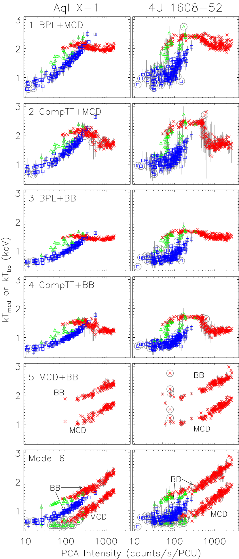
Figure 6.— Variation of the temperature of the thermal component ($kT_{\rm bb}$ for BB and $kT_{\rm mcd}$ for MCD) with the PCA intensity. Cold-seed-photon solutions are shown for Models with CompTT.

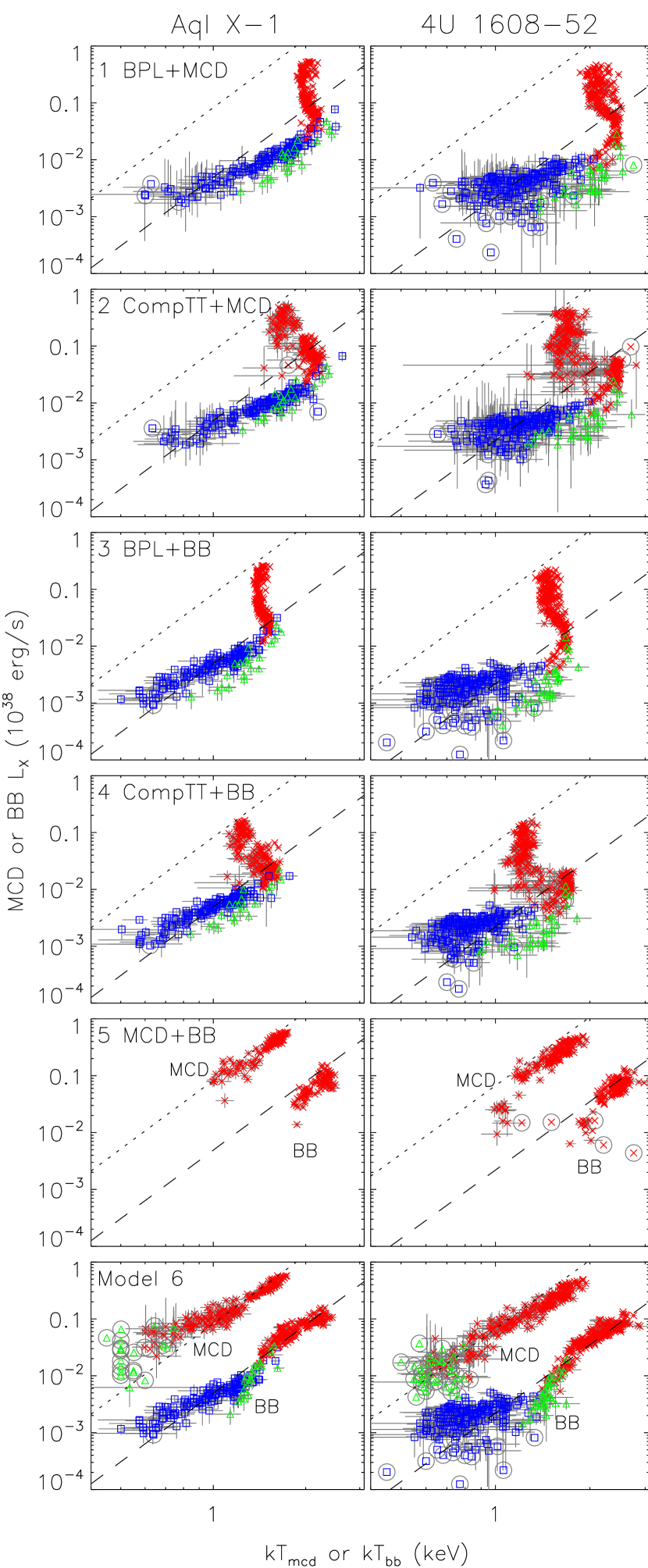
Figure 7.— The luminosity of the thermal component versus its characteristic temperature. Models 5 and 6 produce luminosity evolution for BB and MCD components in the soft state (red crosses) that are nearly parallel to reference lines, which show $L_{\rm X}\propto T^{4}$ with constant emitting surface area. The dotted lines correspond to the NS burst radii (§4.2.2) and the dashed lines correspond to $R=$ 1.9 km and 1.3 km for Aql X–1 and 4U 1608–52, respectively, assuming $L_{\rm X}=4\pi R^{2}\sigma T^{4}$.

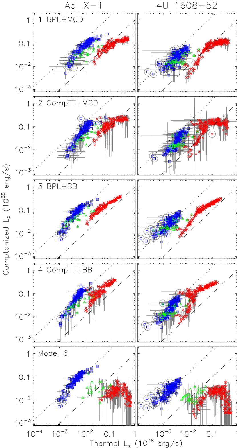
Figure 8.— The luminosity of the Comptonized component versus the luminosity of the thermal component(s). The dashed and dotted lines are for reference. They connect the points where the ratio of the luminosities of the thermal component and the Comptonized component is 1.0 and 0.07, respectively. The latter is a typical value for the hard state.

We fitted the observations of Aql X-1 and 4U 1608-52 using Models 1–4 in Table 2. The PCA does not allow us to gain meaningful constraints on the properties of the (cool) thermal components using the hot-seed-photon models, as explained above. Thus, for models with CompTT, we just show results of cold-seed-photon solutions. In these models, $kT_{\rm s}\ll kT_{\rm e}$ ($kT_{\rm e}$ is typically 2–3 keV in the soft state and several tens of keV in the hard state), and $kT_{\rm s}$ is far below the PCA energy limit. Thus, the Wien approximation of the input seed photon is valid.

The top four rows in Figures 6, 7 and 8 show the fit results for the commonly used Comptonized + thermal models. They correspond to Models 1, $2_{\rm cold}$, 3, and $4_{\rm cold}$ in Table 2, where we also list the mean $\chi^{2}_{\nu}$ values. The errors represent 90$\%$ confidence limits for a single parameter, and the circled points are those with relatively large errors. There is not only strong similarity between these two sources, but also strong similarity between the results of these four models. The extreme difference of the hard and soft states can also be seen in these plots.

Figure 6 shows the variation of the color temperature of the thermal components ($kT_{\rm bb}$ for BB and $kT_{\rm mcd}$ for MCD) with the PCA intensity. All four models show that the temperature of the thermal components of both sources increases with intensity in the hard state. In contrast, the temperature is almost constant (for models with BPL) or decreases (for models with CompTT) with increasing luminosity in the soft state.

Figure 7 shows the luminosity of the thermal component versus its color temperature, $kT_{\rm bb}$ or $kT_{\rm mcd}$. For reference, we also show the lines for constant radius, assuming $L_{\rm X}=4\pi R^{2}\sigma T^{4}$. The NS radii (§4.2.2) are shown with dotted lines in this figure. The dashed lines correspond to $R=$ 1.9 km and 1.3 km for Aql X-1 (catalog ) and 4U 1608-52 (catalog ), respectively; they are derived from the fit to the BB radius values obtained from Model 6 (see below). With increasing luminosity in the respective thermal component, $R_{\rm mcd}$ or $R_{\rm bb}$ increases in the soft state. For the case of MCD-related Models 1 and $2_{\rm cold}$, this behavior in the soft state contradicts the basic prediction of the accretion disk model and warrants the “L” problem in Table 2. Besides, from the comparison with the $R_{\rm burst}$ lines, we find that the inner disk radius $R_{\rm mcd}$ in the hard state and some part of the soft state is simply too small, even after taking into account expected correction factors (see §6). This is consistent with the results of Gierliński & Done (2002b) and Church & Balucińska-Church (2001). Thus, the “R” problem also applies to these two models.

For BB-related Models 3 and $4_{\rm cold}$, the luminosity evolution of the effective radius is tied to the evolution of the boundary layer, which is much less certain. This is why the “L” problem is not applied to the BB component in Table 2. If we attribute the thermal component BB to the boundary layer, it would imply that the boundary layer is measured with almost constant surface area in the hard state, but it spreads out with constant color temperature in the soft state. One possible explanation for the constant color temperature during the spreading of the boundary layer is that the local flux reaches the Eddington limit. The spreading layer model (Suleimanov & Poutanen, 2006) predicts that the color temperature of the boundary layer is $\sim$ 2.4 keV for a NS with $R_{\rm ns}=15$ km and $M=1.4M_{\sun}$ and solar composition of the accreting matter (smaller $R_{\rm ns}$ would predict higher value). A problem with this interpretation for our results of Model 3 or $4_{\rm cold}$ is that the critical value of the temperature for area expansion is $\sim$ 1.5 keV. Higher temperatures are only seen during Type I X-ray bursts from these two sources with maxima normally $>2.5$ keV. Thus, the critical value of the temperature $\sim$ 1.5 keV from Models 3 and $4_{\rm cold}$ does not match expectations for boundary layer spreading. We will show later that these two models are also disfavored from strong similarities of the timing properties between BH and NS LMXBs.

In Figure 8 we investigate the luminosity evolution of the Comptonized component (BPL or CompTT) versus the thermal component(s) (BB or MCD or their sum if both are used). For the thermal component the bolometric luminosity is used while for the Comptonized component we integrated from 1 keV to 200 keV for CompTT and from 1.5 keV to 200 keV for BPL. The 1.5 keV lower limit for the BPL integration is chosen so that this component does not extend below the temperature of the MCD in the soft state, i.e., when the BPL is steep and the lower limit matters. The errors of the luminosity of BPL, CompTT and MCD primarily depend on the uncertainties in their respective normalizations. In Figure 8 we also show two reference lines: dashed and dotted. They connect the points where the ratio of the luminosities of the thermal component and the Comptonized component is 1.0 and 0.07, respectively. The latter is a typical value for the hard state. In both the hard and soft states, the luminosity of the Comptonized component increases with the luminosity of the thermal component, but the two states follow different tracks. In the soft state, the luminosities of these two components are relatively close to each other, while in the hard state, the luminosity of the thermal component is only $\sim 10\%$ of the Comptonized component.

The uncertainties for the thermal-component luminosity from the hot-seed-photon models are quite large from PCA data in the soft state. However, hot-seed-photon models with BB as the thermal component have the “T” problem (§4.2.1). Hot-seed-photon models with MCD as the thermal component have the “L” problem in the soft state (Gierliński & Done, 2002b; Done et al., 2002) and the “R” problem in the hard state from our investigation (not shown).

Since the luminosity evolution of the thermal component in the soft state is either in violation of the basic model (MCD) or, at best, suspicious (BB), we continued to investigate alternative models such as those in the next section.

4.3. Double Thermal Models

Figure 9.— The unfolded spectra and residuals of two sample soft-state observations of Aql X–1 using Model 6. The total model fit is shown as a solid line, the MCD component as a dotted line, the BB component as a dashed line, the CBPL component as a dot-dot-dashed line, and the Gaussian line as a dot-dashed line. The high-$L_{\rm X}$ observation is the same as the sample soft-state observation seen in Figures 4 and 5. The low-$L_{\rm X}$ observations is on 1999 June 3 (hard color 0.32, intensity 243 counts/s/PCU).

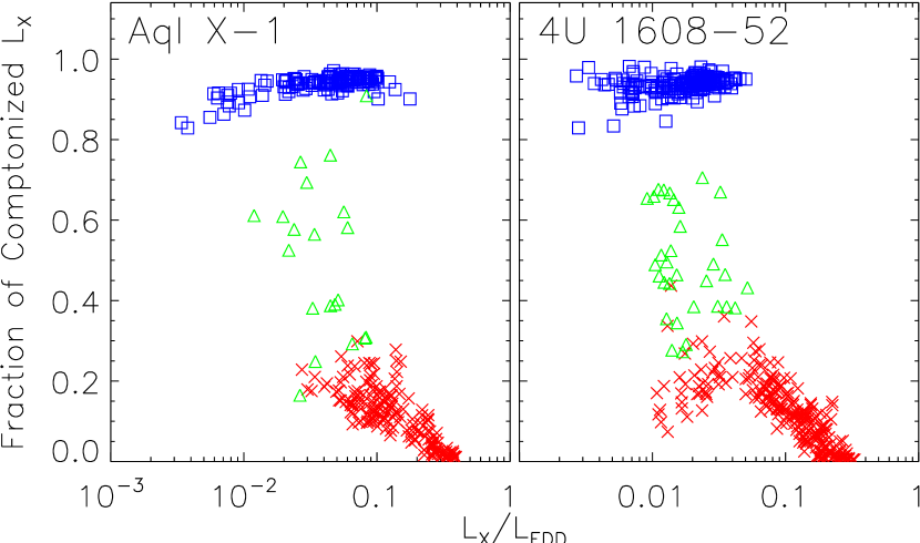
Figure 10.— The fraction of Comptonized luminosity versus the total luminosity, using Model 6. $L_{\rm EDD}=1.8\times 10^{38}$ erg/s, assuming $M_{\rm ns}=1.4M_{\sun}$ for both sources.

Early analyses of NS spectra in the soft state considered the possibility that we might detect thermal components from both the disk and boundary layer (Mitsuda et al., 1984). This “double thermal” model (i.e., MCD+BB or Model 5 in Table 2) was applied to the soft-state observations of Aql X-1 (catalog ) and 4U 1608-52 (catalog ), and the results are shown in the fifth row of panels in Figures 6 and 7. Data points for this model are omitted when $\chi^{2}_{\nu}$ is $>2$ (only for this model). It turns out that this model works very well in the soft state when the luminosity is high, but with the decreasing luminosity, $\chi^{2}_{\nu}$ becomes large. Either source gives a mean $\chi^{2}_{\nu}$ $\sim$ 1.2 and $\sim$ 3.5 for observations with source intensity $>800$ counts/s/PCU and $<500$ counts/s/PCU, respectively (also see Table 2). However, Model 5 is remarkably successful in its implication that the disk and the boundary layer both remain at constant sizes for a substantial range of luminosity (Figure 7). Moreover, the inferred size of the boundary layer is close to that inferred by Models 3 and $4_{\rm cold}$ for the hard state. The failure of Model 5 for soft-state observations at lower luminosity is apparently due to small levels of Comptonization, since the fit residuals are pointing chronically positive at photon energies above 15 keV (PCA data).

Given the interesting luminosity evolution for the soft state with Model 5 (no Comptonization), we added a weakly Comptonized component, while continuing to assume that both the MCD and BB are visible in the soft state. The difficulty here is how to model weak Comptonization by adding a third component. Freely adding a BPL or CompTT component is obviously not feasible, because BPL or CompTT plus one thermal component is sufficient to model the entire spectrum as shown by Models 1–4. As a first attempt, we tried several forms of constrained CompTT (e.g., couple $kT_{\rm s}$ to $kT_{\rm bb}$ or $kT_{\rm mcd}$; force $kT_{\rm e}>10$ keV; or do both), but the fits always yielded large fractions of Comptonization for low-luminosity observations in the soft state. This problem could be due to RXTE’s lack of low-energy coverage.

On the other hand, we found that the entire soft state remains weakly Comptonized if we adopt the following constrained BPL (CBPL) model: the break energy is fixed at 20 keV (the best-fitting break energy is typically $>20$ keV in the hard state and is $\sim 15$ keV in the soft state from Models 1 and 3), and the initial photon index is required to be $\leq 2.5$ (a typical initial photon index in the soft state of BHs is also about 2.5; Remillard & McClintock, 2006). Therefore, we define Model 6 as follows: the hard state is still modeled by BPL+BB (no BPL constraints; same as Model 3 for the hard state) and the soft/transitional states are modeled by MCD+BB+CBPL. Figure 9 shows the unfolded spectra of two soft-state observations using this model, one at low luminosity and the other at high luminosity.

The bottom row of panels of Figures 6, 7 and 8 show the results obtained for Model 6. Figure 6 shows that with the increase in the intensity, $kT_{\rm bb}$ increases both in the hard and soft states, with the tracks that are clearly separated. The BB temperature reaches a maximum $\sim$ 2.5 keV for Aql X-1 (catalog ) and $\sim$ 3.0 keV for 4U 1608-52 (catalog ), similar to the peak temperatures of Type I X-ray bursts from these two sources (Koyama et al., 1981; Nakamura et al., 1989; Galloway et al., 2006). The temperature at the inner disk radius $kT_{\rm mcd}$ increases from $\sim$ 0.5 to 2.0 keV, also correlated with the intensity.

In Figure 7, we see that Model 6 remarkably produces results where $L_{\rm X}\propto T^{4}$ for both the MCD and BB components in the soft state. Furthermore, the inferred emission areas of the boundary layer from the hard and soft states have essentially the same value. The emission area of the boundary layer is small compared with the size of the NS. We realize that the size of the BB emission area slightly increases with decreasing luminosity in the hard state, especially for 4U 1608-52 (catalog ). However, we note that the BB curve lies well below the line of $R_{\rm burst}$ at all luminosities.

In Figure 8, we show the luminosity of the Comptonized component versus the total luminosity of the double thermal components. The behavior in the soft state for Model 6 is quite different from that in the first four models. Here, with increasing luminosity of the thermal components (i.e. $L_{\rm bb}+L_{\rm mcd}$), the luminosity of the Comptonized component first increases and then decreases. At the highest luminosities, the Comptonized component is negligible, as implied by the success of Model 5 in the same region. Figure 10 shows the fraction of the Comptonized luminosity versus the total luminosity. It looks similar to the color-intensity diagram in Figure 2, suggesting that the hard color tracks the degree of Comptonization fairly well.

It should be noted that there are other kinds of weak-Comptonization approximations like constrained power-law (photon index $<2.5$) or constrained cutoff power-law (photon index $<2.5$ and cutoff energy $>10$ keV) that gave results for the soft state that are similar to those obtained using CBPL. For the hard state, Figures 6–8 show that the Model $4_{cold}$ (CompTT+BB) gives similar results to Model 6 in terms of the properties of the thermal component and the fraction of Comptonization. Model 6 is successful, but there are no claims that it is either a unique solution to the problem, nor an adequate depiction of Comptonization other than the estimate for the fraction of energy related to Comptonization.

5. TIMING PROPERTIES AND COMPARISON WITH BLACK HOLES

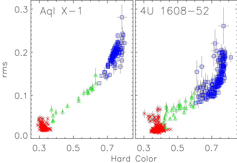
Figure 11.— The integrated rms power in the power density spectrum (0.1–10 Hz and energy band 2–40 keV) versus the hard color.

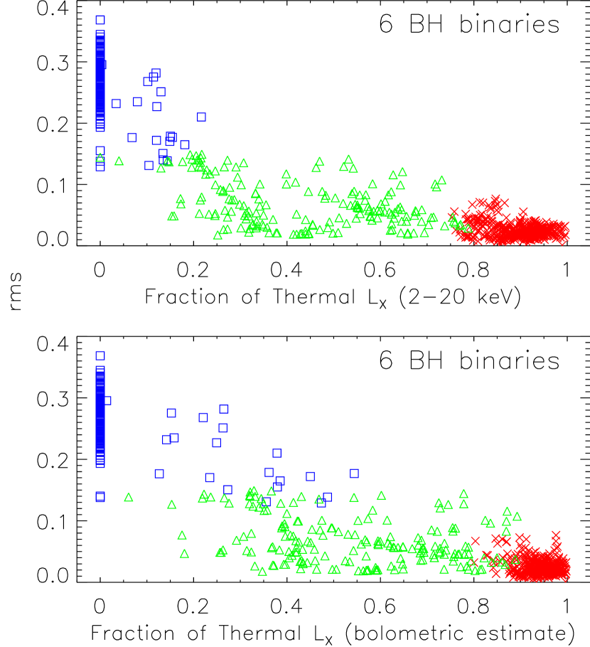
Figure 12.— The integrated rms power versus the fraction of luminosity contained in the thermal (MCD) component for 6 black hole systems.

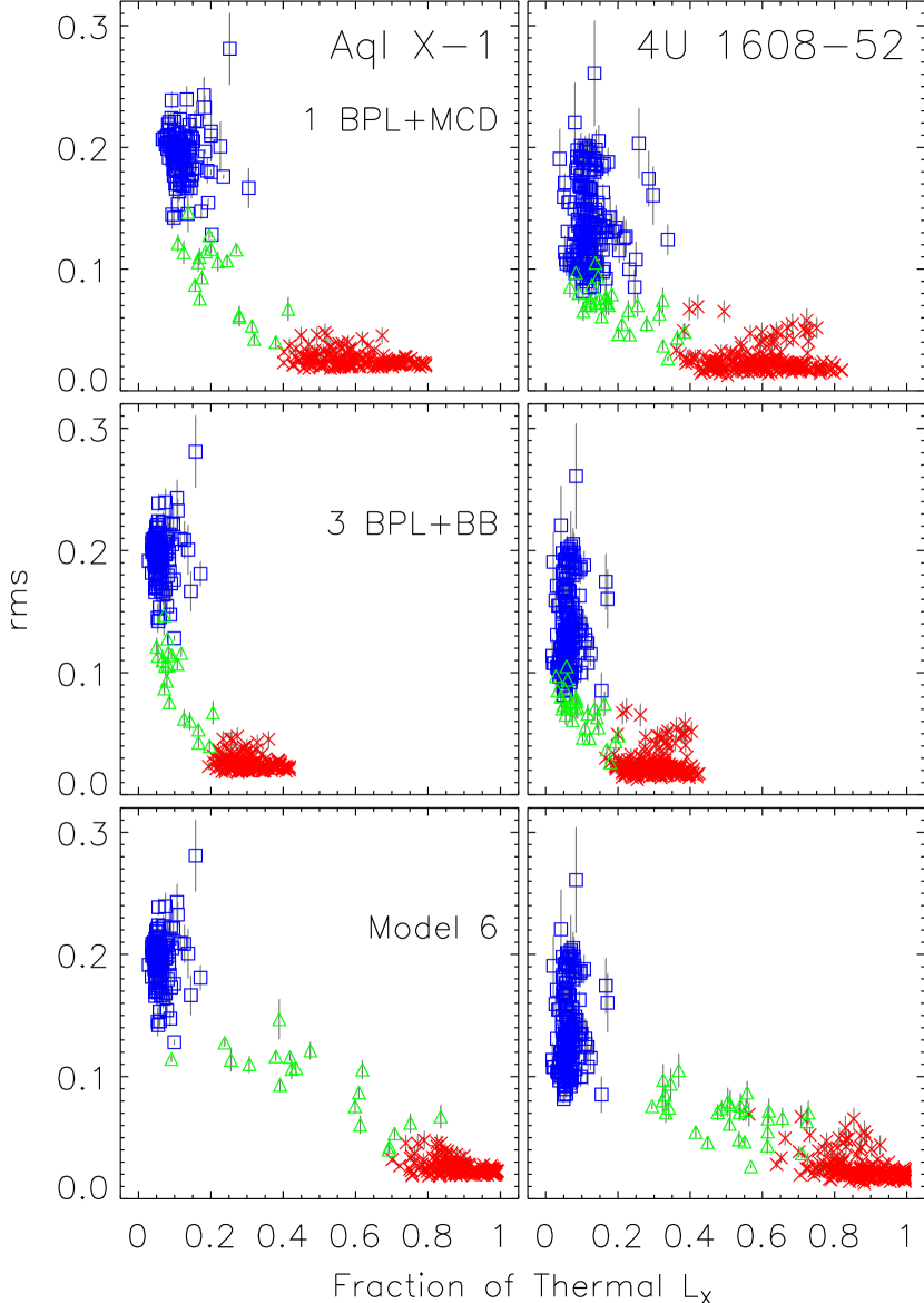
Figure 13.— the rms versus the fraction of luminosity contained in BB and/or MCD components as evaluated for different spectral models.

Compared to Models 1–4, the use of a double thermal model + CBPL (i.e., Model 6) for Aql X-1 (catalog ) and 4U 1608-52 (catalog ) produces dramatically different results for the luminosity evolution of the thermal components in the soft state and for the implied significance of Comptonization in the soft state.

There are strong similarities in timing properties between the BH and NS LMXBs (see, e.g., Wijnands (2001)), which can be used to further assess these differences. In Figure 11, we show the integrated root-mean-square (rms) power in the power density spectrum (0.1–10 Hz and energy band 2–40 keV) versus the hard color for Aql X-1 (catalog ) and 4U 1608-52 (catalog ). The two sources show very similar timing properties. The rms, normalized to a fraction of the source’s mean count rate, is very small ($\lesssim 0.05$) in the soft state, and the values increase with the hard color progressing through the transitional and hard states. The rms versus hard-color relations from Figure 11 can be compared with similar plots for BHs in Remillard & McClintock (2006) (panels g in their Figures 4–9). Based on such a comparison we conclude that, when considered in a model-independent manner, the way in which the strength of the X-ray variability changes as a function of spectral hardness is very similar for BHs and our two NS transients. Since the hard color effectively traces the fractional contribution of the thermal and Comptonized components to the X-ray spectrum in BH systems, it is interesting to see which of our spectral models conserves this similarity when rms is plotted versus the fractional contribution of the thermal component(s).

In Figure 12 we present such a plot for the same 6 BH binaries analyzed by Remillard & McClintock (2006). Two different integration limits were investigated for the thermal and Comptonized luminosities, but the overall behavior was insensitive to our exact choice. It can be seen that for BHs in the soft state, the luminosity fraction of the thermal component is quite high ($\gtrsim 75\%$) and the rms is very small $\lesssim 0.05$. For Aql X-1 (catalog ) and 4U 1608-52 (catalog ) we plot the rms versus the fraction of thermal luminosity for Models 1, 3, and 6 in Figure 13. Note that in case of Model 6 the sum of MCD and BB was used to determine the fractional contribution of the thermal components. Comparing Figures 12 and 13 one can see that only Model 6 reproduces the same dependence of rms on fractional thermal luminosity for Aql X-1 (catalog ) and 4U 1608-52 (catalog ), as for the six BHs. In Models 1 and 3, the luminosity fraction of the thermal component can be as low as 40$\%$ and $20\%$, respectively, while continuing to show very low values of rms power. Similar results are obtained for Models 2 and 4 (cold and hot included for both cases). Hence, for the models outlined in Table 2 only Model 6 links weak Comptonization with low rms power, as is clearly evident in the properties of BHs. Models 1–4 for the soft state are therefore described as having the “P” problem (see §4.2.2 and Table 2).

6. PHYSICAL INTERPRETATIONS OF MODEL 6 FOR THERMAL COMPONENTS

Since Model 6 has many attractive advantages over the other models, we further explore its implications in terms of the physical properties of the accretion flow in both the hard and soft states.

There is a well known difficulty in deriving true radii from the apparent dimensions (i.e., $R_{\rm bb}$, $R_{\rm burst}$, and $R_{\rm mcd}$ extracted from model components of the X-ray spectrum BB, BB_burst, and MCD, respectively). Nevertheless, the small value of $R_{\rm bb}$ and the nearly constant values of $R_{\rm bb}$ and $R_{\rm mcd}$ across a large range in luminosity motivate cautious efforts to discuss physical interpretations.

If we assume the BB emission area to be a latitudinally symmetric equatorial belt, then the BB emission area of the belt should be

$$A_{\rm belt}=4\pi N_{\rm bb}D^{2}_{10\rm kpc}f^{4}k(i,\delta)\ {\rm km}^{2},$$ (1)

where $N_{\rm bb}=R^{2}_{\rm bb}/D^{2}_{10\rm kpc}$ is the normalization of the BB component (isotropic assumption), $f$ represents a spectral hardening factor (sometimes expressed as the ratio of the color to effective temperature), and $k$ is a geometrical correction factor taking into account the emitting geometry and any occultations by the accretion stream. The $k$ factor depends on the disk inclination ($i$), the latitude range (from the NS equator) of surface emission ($\delta$). We note that this factor is also strongly dependent on the properties of the occulting accretion stream. Unless otherwise indicated, we assume a geometrically thin but optically thick accretion stream so that the half belt on the other side of the accretion stream is invisible to the observer. To have some sense of this $k$ factor, we give two examples: $k(i=60\arcdeg,\delta=10\arcdeg)=1.69$, and $k(i=60\arcdeg,\delta=90\arcdeg)=1.33$. From this perspective, the area of the NS, e.g., for Aql X-1 (catalog ) in this study is:

$$A_{\rm ns}=4\pi N_{\rm burst}D^{2}_{10\rm kpc}f^{4}k(i,\delta=90\arcdeg)\ {\rm km}^{2},$$ (2)

assuming that the entire NS surface is radiating (using the asymptotic value of $R_{\rm burst}$ late in the burst). This expression conveys the difficulty in gaining accurate inferences of NS sizes from X-ray burst measurements. The raw values for $R_{\rm burst}$ given in §4.2.2 ignore $f$ and $k$.

Perhaps of greater interest is the effort to understand a key measurement result of this paper: $R_{\rm bb}/R_{\rm burst}\simeq 0.25$ ($N_{\rm bb}/N_{\rm burst}\simeq 1/16$) for Aql X-1 (catalog ). If we assume that the $f$ values cancel in these different applications of the BB model and use the fact $A_{\rm belt}/A_{\rm ns}=\sin\delta$, we obtain

$$\sin\delta = \frac{N_{\rm bb}k(i,\delta)}{N_{\rm burst}k(i,\delta=90\arcdeg)}=\frac{k(i,\delta)}{16k(i,\delta=90\arcdeg)}.$$ (3)

In this case, the $R_{\rm bb}/R_{burst}$ value is equivalent to an equatorial belt with a half-angle of $\delta_{\rm belt}\simeq 9\arcdeg$ for $i=30^{\circ}$, or $\delta_{\rm belt}\simeq 6\arcdeg$ for $i=60^{\circ}$. We stress that this scaling estimate ignores the annular half width of the occulting stream ($\delta_{\rm stream}$) itself. A more realistic estimate is $\delta_{\rm belt}\gtrsim\delta_{\rm stream}+6\arcdeg$ for $i=60\arcdeg$, implying $k\gg 1$.

Regardless of the details of $\delta$, we must confront the implication of measuring $N_{\rm bb}/N_{\rm burst}\sim 1/16$, noting that $N_{\rm burst}$ is the asymptotic value that should screen out effect of the radius expansion and momentary disruption in the occulting stream (§4.2.2). How is it possible that accreting NSs could maintain an almost uniformly small area of BB emission through hard and soft states that span such a wide range in luminosity (i.e., 0.005 to 0.5 $L_{\rm EDD}$)? Such simple results suggest a picture in which a geometrically thin accretion stream feeds a rather well-defined impact zone, where the accreting gas may efficiently release energy before spreading over the remainder of the NS surface. Since the scale height of the inner accretion disk is expected to increase with the accretion rate, it is difficult to understand our results without the help of an inner-most stable circular orbit (ISCO). As illustrated for BHs, the effective potential of an ISCO creates a pinch on the vertical structure of the accretion stream that can suppress variations in the scale height of the inner disk (Abramowicz et al., 1978). To the extent that Model 6 remains viable with further scrutiny, the small size of $R_{\rm bb}$ over a large range in luminosity should be examined as a means to infer that these NSs lie within their ISCOs. This may provide another observational link to general relativity, while providing potential constraints on the NS equation of state.

The ability of Model 6 to restore the expected luminosity evolution of the MCD component motivates efforts to compare the MCD radius and relative luminosity to the results determined for the BB component. In Figure 7, it is evident that the raw values of $R_{\rm mcd}$ are only slightly less than the values of $R_{\rm burst}$ (dotted line) for Aql X-1 (catalog ) and 4U 1608-52 (catalog ). Given the uncertainty in the different correction factors that must be applied, respectively, to the disk and the burst radii in order to derive physical sizes, our results may still be consistent with expectations framed by the preceding discussion, i.e., that $R_{\rm ns}<R_{\rm isco}\lesssim R_{\rm disk}$.

The comparison of BB and MCD luminosities is a trickier topic. The apparent luminosity of the boundary layer ($L_{\rm bb}$) is about one third of that of the disk ($L_{\rm mcd}$) in the soft state, neglecting the weak Comptonization. In contrast, we might expect $L_{\rm bb}\gtrsim L_{\rm mcd}$ if the boundary layer is inside the NS ISCO, as sketched above, where the accreting material may impact the surface with a large relative velocity that includes a component along the radial path. We note, however, that while $L_{\rm mcd}$ is estimated in a true bolometric sense, this is not the case for $L_{\rm bb}$. We need to correct $L_{\rm bb}$ by $k(i,\delta)$ (Equation 1) due to the geometry of the boundary layer and occultation by the accretion stream. For Aql X-1 (catalog ), it is $\simeq 1.7$ ($i=60\arcdeg$) or $\simeq 2.6$ ($i=30\arcdeg$), and these factions can become much larger if $\delta_{\rm stream}\sim\delta_{\rm belt}$, as noted above. We conclude that there is considerable uncertainty in our final results as to whether the total energy losses at the boundary layer are less than the total bolometric luminosity of the other spectral components.

7. PHYSICAL CONSEQUENCES OF MODEL 6 FOR THE HARD STATE

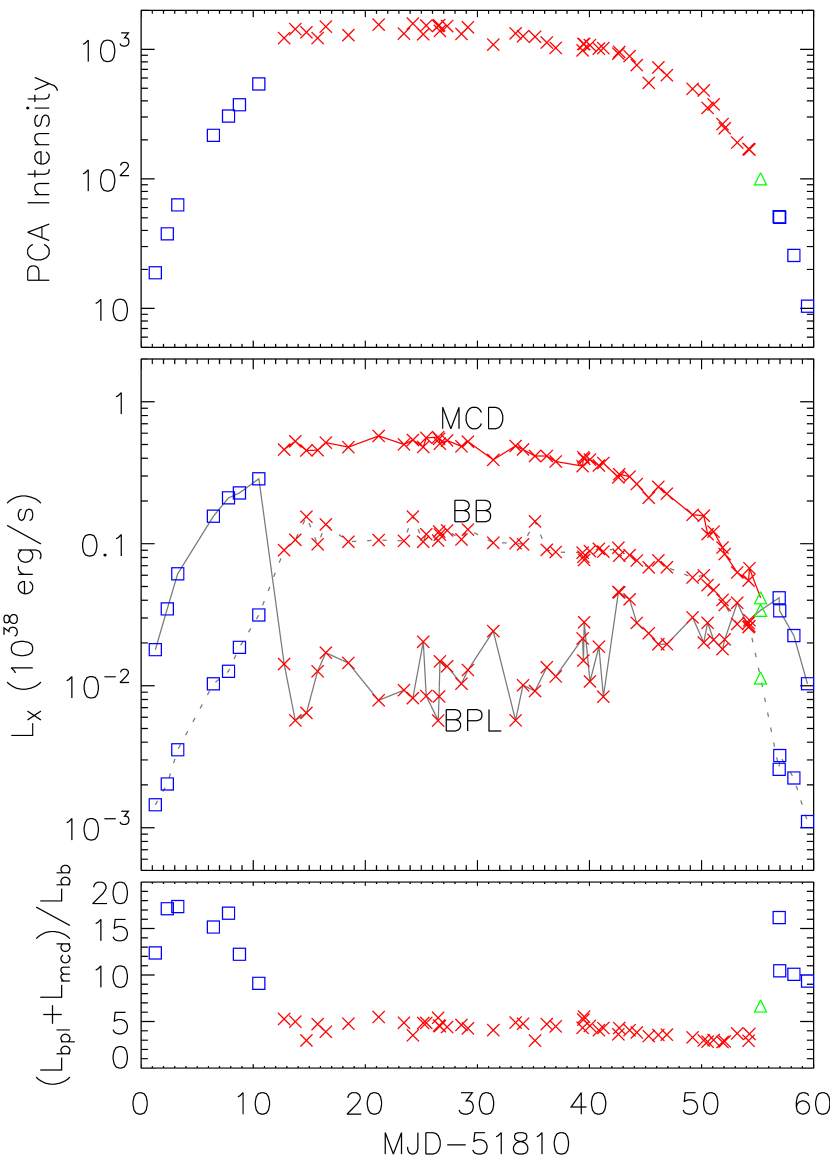
Figure 14.— The luminosity evolution of different spectral components (middle panel) during the 2000 outburst of Aql X–1, as viewed with Model 6. Blue, green, and red symbols denote hard, transitional, and soft states, as done previously. Note that the MCD component (points connected by a solid red line) is not directly visible with the PCA in the hard state. The top panel shows the PCA count rate (2-30 keV). The bottom panel shows the ratio: ($L_{\rm bpl}+L_{\rm mcd}$) / $L_{\rm bb}$, and the value is clearly highest in the hard state, when Comptonization appears to dominate the X-ray spectrum.

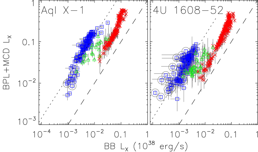
Figure 15.— The luminosity of non-BB components (i.e., BPL+MCD) versus the luminosity of the BB component. At the transitional BB luminosity that separates hard and soft states, the hard-state BPL appears to be very luminous compared to the soft-state MCD. The two reference lines, dashed and dotted lines, connect the points where the ratio of the luminosities of the BB component and the non-BB components is 1.0 and 0.07, respectively.

Figure 14 shows the luminosity evolution with time during a well-covered outburst of Aql X-1 (catalog ) in 2000. The light curve of this outburst is shown on the top panel. The middle panel shows the luminosity evolution of each spectral component, using our hybrid Model 6, where the BPL and MCD dominate the apparent luminosity of the hard and soft states, respectively. The bolometric BB luminosity ($L_{\rm bb}$) curve resembles the total luminosity curve, and it provides a reference measurement that allows us to further compare the hard and soft states. The ratio of BPL (isotropic) and MCD (bolometric) luminosities ($L_{\rm bpl}+L_{\rm mcd}$) to $L_{\rm bb}$ is shown in the bottom panel. We note that the values of this ratio are elevated, in part, by the $k$ factor described for Eq. 1. Nevertheless the high luminosity of the hard state, relative to $L_{\rm bb}$, is apparent in the bottom panel of Figure 14.

To compare the hard and soft state luminosities in a more global manner, Figure 15 shows ($L_{\rm bpl}+L_{\rm mcd}$) versus $L_{\rm bb}$ for all of the RXTE observations of Aql X-1 (catalog ) and 4U 1608-52 (catalog ). The behavior of these two sources is quite similar. The states are largely separated by vertical lines near (uncorrected) $L_{\rm bb}\sim 10^{36}$ erg/s. Here, the hard-state values for ($L_{\rm bpl}+L_{\rm mcd}$) are clearly higher than those for the soft state, by a factor of $\sim 6$. For the hard state, the vertical axis represents Comptonization, since $90\%$ of the total luminosity in the hard state is due to $L_{\rm bpl}$. In the soft state, the vertical axis is effectively the disk luminosity. On the horizontal axis, we assume that $L_{\rm bb}$ represents emission from the boundary layer, and we can then use the nearly constant value of $R_{\rm bb}$ across the hard and soft states to motivate the presumption that $L_{\rm bb}$ quantifies the mass accretion rate onto the NS surface. Using these assumptions, there are still different ways to interpret Figure 15.

First, if we further assume that the total accretion rate ($\dot{M}$) flows into a boundary layer with constant $\delta_{\rm belt}$, then $L_{\rm bb}$ effectively tracks ($\dot{M}$), and we can compare hard and soft states in terms of their radiation efficiency. Unlike $L_{\rm bb}$, $L_{\rm mcd}$ and $L_{\rm bpl}$ are not expected to require large correction factors, although the origin of the BPL is very uncertain. We would then conclude from Figure 15 that Comptonization in the hard state has higher radiative efficiency than thermal disk emission in the soft state, and this occurs across a wide range in the accretion rate. This idea is a radical departure from expectations.

Alternatively, we can refrain from making assumptions about $\dot{M}$, and choose a line of constant ($L_{\rm bpl}+L_{\rm mcd}$) in Figure 15. Quite generally, then, one would conclude that less mass reaches the NS surface in the hard state, compared to the soft state, for a given level of luminosity on the vertical axis. This might suggest that the majority of the mass flow is disrupted from the normal path to the NS in the hard state. Given the expectation for radio jets in the hard state of accreting NS LMXBs (e.g., Fender, 2006; Migliari & Fender, 2006), this could further imply that a significant fraction of mass accretion in the hard state is redirected to outflow in the jet. The energy source for this scenario could be problematic.

Finally, it is also possible that some of our preliminary assumptions are incorrect. Changes in accretion geometry across the state boundary, e.g., from correlated jumps in $\delta_{\rm belt}$ and $\delta_{stream}$, would be one way to invalidate the assumption that $L_{\rm bb}$ uniformly tracks the NS surface accretion rate across both states. All of these ideas need to be investigated for other sources and in different ways.

8. SUMMARY AND DISCUSSION

We have analyzed ten years of RXTE observations of two NS X-ray transients, Aql X-1 (catalog ) and 4U 1608-52 (catalog ), through more than twenty individual outbursts. Although there is much variety in these outbursts, the spectral and timing properties are well organized, as has been demonstrated in previous investigations (Muno et al., 2002; Gierliński & Done, 2002a). It is also well known that several different models may adequately fit the X-ray spectra of NS LMXBs, while each one may convey very different physical implications, e.g., the temperatures and sizes of the emitting regions. We therefore attempted to design performance-based criteria for evaluating these models, hoping to gain insights on a model’s self consistency, while taking advantage of the large data archive for these two atoll-transient prototypes.

Among these criteria, there is an important quantity, which is the energy fraction for Comptonization, i.e., how much energy is directly visible as pure thermal radiation and what remaining fraction is diverted and expressed as inverse Compton radiation. This quantity is interesting from an accretion-energetics point of view. It can be calculated from any of these models, and furthermore, it is the gateway for comparing NSs and BHs in terms of the relationship between energetics and the measured timing properties.

First we examined the classical two-component models with a Comptonized component (BPL or CompTT) and a thermal component (MCD or BB). We confirmed that many combinations can describe the X-ray spectra successfully. Moreover there are two possible seed-photon solutions for models that utilize CompTT, a problem that is also present for instruments with extended low-energy coverage like BeppoSAX. In the soft state, the two-component models behaved poorly for a variety of reasons shown in Table 2, Figure 7, and Figures 12–13. We then progressed to consider a double-thermal model (MCD+BB) for the soft state, and we found a need to account for weak Comptonization at the low-$L_{\rm X}$ end of the soft-state track. We then devised a hybrid “Model 6” in which the hard state is modeled by BB+BPL while the soft state is modeled by MCD+BB+CBPL, where the third component is a constrained BPL ($E_{\rm b}=20$ keV and $\Gamma_{1}\leq 2.5$) that can assume the role of weak Comptonization.

It turns out that Model 6 offers three great advantages over the classical Comptonized + thermal Models. (1) It produces an $L_{\rm X}\propto T^{4}$ relation for both the MCD and BB in the soft state with a sufficiently large value for the inner disk radius (compared to the NS radius inferred from Type I bursts). (2) The emission area of the BB extends from the hard to the soft state with essentially the same value. (3) The fraction of Comptonization inferred by this model is also consistent with that for BHs for given values of rms power in the power density spectra. When BH binaries are in the thermal state, the Comptonization fractions in the energy spectra are very low and the rms power is also very low, rms $<0.05$. Atoll sources in the soft state show similar rms values, but only Model 6 implies low Comptonization for the soft state.

With regard to previous investigations of NS X-ray spectra (§1), our Model 6 splices together the Western model for the hard state (BB + a heavily Comptonized disk) and a three-component model for the transitional and soft states (BB + MCD + constrained BPL) that represents a BB plus a very weakly Comptonized disk. The soft-state portion of this model was heavily influenced by the original version of the Eastern model (Mitsuda et al. 1984). We further note that low Comptonization solutions ($\tau\sim 1$; $kT_{\rm e}>20$ keV) for the soft state were derived with a two-component Eastern model for 4U 1608-52 (catalog ) with Tenma data (Mitsuda et al. 1989), and these are the closest results that we can find to those (soft state) of Model 6.

The ad hoc scheme in Model 6 to handle weak Comptonization with the CBPL component for the soft state is obviously a topic that needs further work. Model 6 for the soft state is a three-component continuum model. We did not try to test three-component models in an open-handed manner. Instead, we focused on low-Comptonization solutions, progressing from the success of Model 5 (no Comptonization). The CBPL used in this paper is just one possible solution; our investigation showed that constrained power-law with photon index $<2.5$ or constrained cutoff power-law with photon index $<2.5$ and cutoff energy $>10$ keV would also produce similar results to those obtained with the CBPL. As other alternatives, we tried to add a constrained version of CompTT to the two thermal components, by coupling $kT_{\rm s}$ to $kT_{\rm bb}$ or $kT_{\rm mcd}$, or requiring $kT_{\rm e}>10$ keV, or doing both. However, the fits always yielded very strong Comptonization in the low-luminosity soft state, but the fit residuals for Model 5 suggested that only weak Comptonization is present in the low-luminosity soft state. This could be due to the limited low-energy coverage of RXTE data. We investigated BeppoSAX, which has extended low-energy coverage, for possible new insight. Unfortunately, each X-ray source has only one soft-state observation from BeppoSAX, and both of them are at high luminosity. Future observations with broad-band instruments like Suzaku could be important to this issue. As for the hard state, Model 6 uses BB+BPL. Replacement of BPL with CompTT does not change our conclusions for the properties of the BB component and the fraction of Comptonization as long as the cold-seed-photon solution is used.

There is a question of whether we could also see a thermal disk in the hard state, where the trend from Figure 8 would imply $kT_{\rm mcd}\lesssim$ 0.5 keV. Such disks have in fact been observed in the hard state of a number of BH X-ray transients (Miller et al., 2006a, b; Rykoff et al., 2007), with instruments that have better sensitivity at low energies than RXTE. However, being able to detect these components in NSs is not only a matter of low-energy sensitivity. One also needs a relatively low interstellar absorption. Moreover, in NSs a disk would not be the only thermal component contributing around 0.5 keV, since there is also emission from the boundary layer, and it is difficult to disentangle the contribution from the two components at low luminosities when the spectrum is not dominated by these thermal components.

If the boundary layer is an equatorial belt of BB emission, then Model 6 implies that the visible surface area of the belt remains nearly constant, with $N_{\rm bb}/N_{\rm burst}\sim 1/16$, over a wide range in $L_{\rm X}$ (0.005–0.5 $L_{\rm Edd}$). Current theories predict that the geometry and physical processes in the boundary layer should vary significantly with $L_{\rm X}$ (e.g., Inogamov & Sunyaev, 1999; Popham & Sunyaev, 2001; Kluzniak & Wagoner, 1985), and some observations have been interpreted in such a manner (Church et al., 2002). Our results are much simpler than expected, suggesting that a geometrically thin accretion stream impacts a rather well-defined surface area, where the gas radiates efficiently before spreading over the NS. This scenario would seem to require that the NS lies within its ISCO, which pinches the vertical structure of the accretion stream (Abramowicz et al., 1978) as it flows toward the NS. This topic must be investigated in further detail.

Table 1X-ray Sources and Observations Prior to 2006 January 1

	number of total/used	Time of total/used	NH	Distance
Source name	observations	observations (ks)	($10^{22}{\rm cm}^{-2}$)	(kpc)
Aql X-1 (catalog )	393/333	1402/1252	0.5	5
4U 1608-52 (catalog )	523/459	1310/1204	1.0	3.6

Table 2The spectral models

	Hard State				Soft/Transitional State
Model #	Description	$\chi^{2}_{\nu}$($\sigma$)	Problems		Description	$\chi^{2}_{\nu}$($\sigma$)	Problems
1	BPL+MCD	0.93(0.21),0.88(0.16)	R		BPL+MCD	0.99(0.38),1.07(0.36)	R L P
$2_{\rm cold}$	CompTT+MCD	1.00(0.28),0.90(0.17)	R		CompTT+MCD	1.04(0.39),0.93(0.25)	R L P
$2_{\rm hot}$	CompTT+MCD	…	R		CompTT+MCD	…	L P
3	BPL+BB	0.94(0.21),0.90(0.17)	—		BPL+BB	1.06(0.41),1.24(0.49)	P
$4_{\rm cold}$	CompTT+BB	0.99(0.24),0.93(0.19)	—		CompTT+BB	0.95(0.33),0.90(0.25)	P
$4_{\rm hot}$	CompTT+BB	…	T		CompTT+BB	…	T P
5	…	…	…		MCD+BB	1.23(0.36),1.17(0.38)	…
6	BPL+BB	0.94(0.21),0.90(0.17)	—		MCD+BB+CBPL	1.15(0.30),1.02(0.27)	—

Note. — All models also include an interstellar absorption component and a Gaussian line. The notations BPL, MCD, BB and CompTT refer the bknpower, diskbb, bbodyrad, and comptt models in XSPEC, respectively. CBPL is a constrained BPL with the break energy $E_{\rm b}$ fixed at $20$ keV and the initial photon index $\Gamma_{1}$ forced to be smaller than $2.5$. “…” means that the information is not available or meaningless because the corresponding model does not work. “—” means that none of the four problems listed in §4.2.2 is found to apply to the corresponding model/spectral state.

Table 3BEST-FITTING PARAMETERS OF TWO SAMPLE SPECTRA

Data	Model	$kT_{\rm s}$ keV	$kT_{\rm e}$ keV	$\tau$	$kT_{\rm mcd},kT_{\rm bb}$ keV	$N_{\rm mcd},N_{\rm bb}$	$\chi^{2}_{\nu}$(d.o.f)
Hard-state sample	CompTT+MCD(cold)	$\lesssim 0.35$	$14.3_{-0.9}^{+1.0}$	$6.07_{-0.36}^{+0.36}$	$1.79_{-0.08}^{+0.07}$	$1.7_{-0.3}^{+0.3}$	$1.49(78)$
Hard-state sample	CompTT+MCD(hot)	$1.16^{+0.08}_{-0.12}$	$15.5^{+1.2}_{-1.0}$	$5.54^{+0.32}_{-0.32}$	$1.00^{+0.05}_{-0.09}$	$44.8^{+17.2}_{-10.7}$	1.32(78)
Hard-state sample	CompTT+BB(cold)	$\lesssim 0.4$	$15.0_{-0.9}^{+1.0}$	$2.53_{-0.14}^{+0.14}$	$1.21_{-0.04}^{+0.04}$	$8.9_{-1.5}^{+1.7}$	$1.25(78)$
Hard-state sample	CompTT+BB(hot)	$1.03_{-0.18}^{+0.12}$	$16.6_{-1.1}^{+1.3}$	$2.24_{-0.14}^{+0.14}$	$0.67_{-0.05}^{+0.05}$	$227.9_{-44.0}^{+63.1}$	$1.59(78)$
Soft-state sample	CompTT+MCD(cold)	$\lesssim 0.5$	$2.5_{-0.1}^{+0.1}$	$16.6_{-2.5}^{+8.5}$	$1.70_{-0.06}^{+0.08}$	$68.7_{-15.7}^{+22.6}$	$1.27(53)$
Soft-state sample	CompTT+MCD(hot)	$1.02_{-0.03}^{+0.02}$	$2.6_{-0.1}^{+0.1}$	$10.1_{-0.3}^{+0.3}$	$\lesssim 0.7$	…	$0.95(53)$
Soft-state sample	CompTT+BB(cold)	$\lesssim 0.5$	$2.5_{-0.1}^{+0.1}$	$6.08_{-0.29}^{+0.25}$	$1.24_{-0.04}^{+0.04}$	$164.1_{-25.4}^{+27.9}$	$1.07(53)$
Soft-state sample	CompTT+BB(hot)	$1.02_{-0.04}^{+0.03}$	$2.6_{-0.1}^{+0.1}$	$4.66_{-0.16}^{+0.16}$	$\lesssim 0.5$	…	$0.95(53)$

Note. — The detailed information of these two spectra are given at the beginning of §4.2.1 and their unfolded spectra are shown in Figures 4 and 5. The notations “cold” and “hot” refer to the cold and hot-seed-photon models respectively (see §4.2.1). For CompTT+MCD models, a spherical geometry was assumed for CompTT component, while for CompTT+BB models, a disk geometry was assumed instead. $N_{\rm mcd}$ and $N_{\rm bb}$ are normalizations (in unit of km² at distance 10 kpc) of MCD and BB, respectively.

References

- Abramowicz et al. (1978) Abramowicz, M., Jaroszynski, M., & Sikora, M. 1978, A&A, 63, 221
- Asai et al. (2000) Asai, K., Dotani, T., Nagase, F., & Mitsuda, K. 2000, ApJS, 131, 571
- Barret (2001) Barret, D. 2001, Advances in Space Research, 28, 307
- Barret & Olive (2002) Barret, D. & Olive, J.-F. 2002, ApJ, 576, 391
- Barret et al. (2000) Barret, D., Olive, J. F., Boirin, L., et al. 2000, ApJ, 533, 329
- Barret et al. (2003) Barret, D., Olive, J. F., & Oosterbroek, T. 2003, A&A, 400, 643
- Bradt et al. (1993) Bradt, H. V., Rothschild, R. E., & Swank, J. H. 1993, A&AS, 97, 355
- Christian & Swank (1997) Christian, D. J. & Swank, J. H. 1997, ApJS, 109, 177
- Church & Balucińska-Church (2001) Church, M. J. & Balucińska-Church, M. 2001, A&A, 369, 915
- Church et al. (2002) Church, M. J., Inogamov, N. A., & Bałucińska-Church, M. 2002, A&A, 390, 139
- Di Salvo et al. (2000a) Di Salvo, T., Iaria, R., Burderi, L., & Robba, N. R. 2000a, ApJ, 542, 1034
- Di Salvo et al. (2000b) Di Salvo, T., Stella, L., Robba, N. R., et al. 2000b, ApJ, 544, L119
- Done & Gierliński (2003) Done, C. & Gierliński, M. 2003, MNRAS, 342, 1041
- Done et al. (2002) Done, C., Życki, P. T., & Smith, D. A. 2002, MNRAS, 331, 453
- Farinelli et al. (2005) Farinelli, R., Frontera, F., Zdziarski, A. A., et al. 2005, A&A, 434, 25
- Fender (2006) Fender, R. 2006, in Compact Stellar X-ray Sources (eds. W. Lewin & M. van der Klis, Cambridge University Press), 381–419
- Galloway et al. (2006) Galloway, D. K., Muno, M. P., Hartman, J. M., et al. 2006, astro-ph/0608259
- Gierliński & Done (2002a) Gierliński, M. & Done, C. 2002a, MNRAS, 331, L47
- Gierliński & Done (2002b) —. 2002b, MNRAS, 337, 1373
- Gilfanov et al. (2003) Gilfanov, M., Revnivtsev, M., & Molkov, S. 2003, A&A, 410, 217
- Guainazzi et al. (1998) Guainazzi, M., Parmar, A. N., Segreto, A., et al. 1998, A&A, 339, 802
- Hasinger & van der Klis (1989) Hasinger, G. & van der Klis, M. 1989, A&A, 225, 79
- Iaria et al. (2005) Iaria, R., di Salvo, T., Robba, N. R., et al. 2005, A&A, 439, 575
- Inogamov & Sunyaev (1999) Inogamov, N. A. & Sunyaev, R. A. 1999, Astronomy Letters, 25, 269
- Jahoda et al. (2006) Jahoda, K., Markwardt, C. B., Radeva, Y., et al. 2006, ApJS, 163, 401
- Jahoda et al. (1996) Jahoda, K., Swank, J. H., Giles, A. B., et al. 1996, in Proc. SPIE Vol. 2808, p. 59-70, EUV, X-Ray, and Gamma-Ray Instrumentation for Astronomy VII, Oswald H. Siegmund; Mark A. Gummin; Eds., ed. O. H. Siegmund & M. A. Gummin, 59–70
- Kluzniak & Wagoner (1985) Kluzniak, W. & Wagoner, R. V. 1985, ApJ, 297, 548
- Koyama et al. (1981) Koyama, K., Inoue, H., Makishima, K., et al. 1981, ApJ, 247, L27
- Kreykenbohm et al. (2004) Kreykenbohm, I., Wilms, J., Coburn, W., et al. 2004, A&A, 427, 975
- Kubota & Done (2004) Kubota, A. & Done, C. 2004, MNRAS, 353, 980
- Levine et al. (1996) Levine, A. M., Bradt, H., Cui, W., et al. 1996, ApJ, 469, L33
- Lewin et al. (1993) Lewin, W. H. G., van Paradijs, J., & Taam, R. E. 1993, Space Science Reviews, 62, 223
- Maccarone & Coppi (2003a) Maccarone, T. J. & Coppi, P. S. 2003a, MNRAS, 338, 189
- Maccarone & Coppi (2003b) —. 2003b, A&A, 399, 1151
- Maitra & Bailyn (2004) Maitra, D. & Bailyn, C. D. 2004, ApJ, 608, 444
- Markoff et al. (2005) Markoff, S., Nowak, M. A., & Wilms, J. 2005, ApJ, 635, 1203
- Migliari & Fender (2006) Migliari, S. & Fender, R. P. 2006, MNRAS, 366, 79
- Miller et al. (2006a) Miller, J. M., Homan, J., & Miniutti, G. 2006a, ApJ, 652, L113
- Miller et al. (2006b) Miller, J. M., Homan, J., Steeghs, D., et al. 2006b, ApJ, 653, 525
- Mitsuda et al. (1984) Mitsuda, K., Inoue, H., Koyama, K., et al. 1984, PASJ, 36, 741
- Mitsuda et al. (1989) Mitsuda, K., Inoue, H., Nakamura, N., & Tanaka, Y. 1989, PASJ, 41, 97
- Muno et al. (2002) Muno, M. P., Remillard, R. A., & Chakrabarty, D. 2002, ApJ, 568, L35
- Nakamura et al. (1989) Nakamura, N., Dotani, T., Inoue, H., et al. 1989, PASJ, 41, 617
- Natalucci et al. (2000) Natalucci, L., Bazzano, A., Cocchi, M., et al. 2000, ApJ, 543, L73
- Olive et al. (2003) Olive, J.-F., Barret, D., & Gierliński, M. 2003, ApJ, 583, 416
- Oosterbroek et al. (2001) Oosterbroek, T., Barret, D., Guainazzi, M., & Ford, E. C. 2001, A&A, 366, 138
- Penninx et al. (1989) Penninx, W., Damen, E., van Paradijs, J., Tan, J., & Lewin, W. H. G. 1989, A&A, 208, 146
- Popham & Sunyaev (2001) Popham, R. & Sunyaev, R. 2001, ApJ, 547, 355
- Reig et al. (2000) Reig, P., Méndez, M., van der Klis, M., & Ford, E. C. 2000, ApJ, 530, 916
- Reig et al. (2004) Reig, P., van Straaten, S., & van der Klis, M. 2004, ApJ, 602, 918
- Remillard et al. (2006) Remillard, R. A., Lin, D., Cooper, R. L., & Narayan, R. 2006, ApJ, 646, 407
- Remillard & McClintock (2006) Remillard, R. A. & McClintock, J. E. 2006, ARA&A, 44, 49
- Rothschild et al. (1998) Rothschild, R. E., Blanco, P. R., Gruber, D. E., et al. 1998, ApJ, 496, 538
- Rutledge et al. (2001) Rutledge, R. E., Bildsten, L., Brown, E. F., Pavlov, G. G., & Zavlin, V. E. 2001, ApJ, 559, 1054
- Rykoff et al. (2007) Rykoff, E. S., Miller, J. M., Steeghs, D., & Torres, M. A. P. 2007, astro-ph/0703497
- Suleimanov & Poutanen (2006) Suleimanov, V. & Poutanen, J. 2006, MNRAS, 369, 2036
- Titarchuk (1994) Titarchuk, L. 1994, ApJ, 434, 570
- van der Klis (2006) van der Klis, M. 2006, in Compact Stellar X-ray Sources (eds. W. Lewin & M. van der Klis, Cambridge University Press), 39–112
- van Straaten et al. (2003) van Straaten, S., van der Klis, M., & Méndez, M. 2003, ApJ, 596, 1155
- White et al. (1988) White, N. E., Stella, L., & Parmar, A. N. 1988, ApJ, 324, 363
- Wijnands (2001) Wijnands, R. 2001, Advances in Space Research, 28, 469