Angular Anisotropies in the Cosmic Gamma-ray Background as a Probe of its Origin

Abstract

Notwithstanding the advent of the Gamma-ray Large Area Telescope, theoretical models predict that a significant fraction of the cosmic $\gamma$-ray background (CGB), at the level of 20% of the currently measured value, will remain unresolved. The angular power spectrum of intensity fluctuations of the CGB contains information on its origin. We show that probing the latter from a few tens of arcmin to several degree scales, together with complementary GLAST observations of $\gamma$-ray emission from galaxy clusters and the blazars luminosity function, can discriminate between a background that originates from unresolved blazars or cosmic rays accelerated at structure formation shocks.

1. INTRODUCTION

The existence of diffuse $\gamma$-ray radiation was established in the early 70’s at the dawn of $\gamma$-ray astronomy by the SAS 2 mission  (Fichtel et al., 1975) and further assessed by COS B (Bennett, 1990). The determination of an extragalactic component (heretofore, CGB for cosmic $\gamma$-ray background), which relies on a model for the foreground Galactic emission, became possible only later with the advent of the Compton Gamma Ray Observatory. At energies above 30 MeV the EGRET experiment onboard the CGRO measured a CGB characterized by a specific intensity $I_{\nu}(\varepsilon)$=$5.4(\varepsilon/{\rm keV})^{-2.1}$ ph cm^-2 s^-1 keV^-1 sr^-1 or an integral intensity above 100 MeV, $I$=$1.45\times 10^{-5}$ ph cm^-2 s^-1 sr^-1 (Sreekumar et al., 1998). A recent reassessment of this measurement changes the spectrum from a straight power law to a convex one and reduces the integral intensity to $1.15\times 10^{-5}$ ph cm^-2 s^-1 sr^-1 (Strong et al., 2004, but see also Keshet et al. 2004).

The origin of the CGB is still subject of debate. One naturally expects a population of unresolved blazars, a class of AGNs known to emit up to the highest energies, to contribute to it (Padovani et al., 1993; Stecker & Salamon, 1996; Mücke & Pohl, 2000). Quantitative estimates, however, remain uncertain and various approaches suggest a contribution of order 25-50% of the CGB (Chiang & Mukherjee, 1998; Narumoto & Totani, 2006). Another candidate mechanism is inverse Compton (IC) emission on CMB photons from cosmic-ray (CR) electrons accelerated at structure formation shocks both around galaxy clusters (GC) and cosmic filaments (Loeb & Waxman, 2000). This process can contribute up to a fraction 20% of the CGB, without violating the existing EGRET upper limits on the $\gamma$-ray emission from individual GCs (Miniati, 2002). Normal and/or starburst galaxies have also been proposed as substantial $\gamma$-ray emitters (Pavlidou & Brian, 2002; Thompson et al., 2007). Contributions from $\pi^{0}$-decay due to CR protons in the core of GCs (e.g., Miniati, 2002; Colafrancesco & Blasi, 1998) and annihilation of dark matter are also possible (e.g., Ando & Komatsu, 2006). Note, however, that except for blazars none of these proposed sources has been detected in $\gamma$-rays as yet.

The Large Area Telescope onboard GLAST will advance our understanding of the origin of the CGB, by improving our estimate of the Galactic emission, by resolving part of the extragalactic component due known $\gamma$-ray populations and, possibly, by detecting new types of $\gamma$-ray sources. According to current theoretical predictions, a significant fraction ($\geq 25\%$) of the CGB will remain unresolved by GLAST. In this Letter we study the angular intensity fluctuations of this residual component as a means to discriminate among viable models for its origin. We consider the case of blazars and CRs accelerated at structure formation shocks. We use numerical simulations to model the relevant quantities involved in the calculations, particularly the correlation function of the sources. We predict a substantial difference in the level of fluctuations in the two scenarios above, testable with GLAST from a few tens of arcmin to several degrees. This experiment, together with improved determinations of the blazar luminosity function and $\gamma$-ray emission from GCs by GLAST, will provide a discriminatory test for the unresolved CGB in the GLAST era. CGB fluctuations due to structure shocks were also computed in Waxman & Loeb (2000) analytically, and for an emission sufficient to account for the whole EGRET CGB. Our work is complementary to that of Ando et al. who, with different methods, studied the fluctuations produced by (a) sources similar to those considered here but resolved by GLAST (2006a), and (b) unresolved emission from blazars and annihilation in dark matter halos (2006b). Finally, CGB fluctuations were also studied by Zhang & Beacom (2004) for MeV emission from SN Ia, and by Cuoco et al. (2006) for nearby emission above $\geq$100 GeV. Note that the success of any of these experiments hinges on the ability to assess and, if necessary, separate out fluctuations of Galactic origin. This requires a study the luminosity function and statistical spatial distribution of Galactic $\gamma$-ray sources similar to the one carried out below for extragalactic sources.

Throughout we assume a $\Lambda$CDM cosmological model with $\Omega_{m}$=0.3, $\Omega_{\Lambda}$=0.7, $\Omega_{b}$=0.04, and $h\equiv H_{0}/100\,{\rm km}\,{\rm s}^{-1}{\rm Mpc}^{-1}$=$0.7$ (Spergel et al., 2003).

2. Model

Given the integral intensity $I(\hat{v})$, above photon energy $\varepsilon_{0}$ and along a direction $\hat{v}$, the angular two point correlation function characterizing the fluctuation $\delta I(\hat{v})\equiv I(\hat{v})-\langle I\rangle_{\Omega}$ about the solid-angle-average value $\langle I\rangle_{\Omega}$, is the ensemble average $C(\theta)$=$\langle\delta I(\hat{v})\delta I(\hat{u})\rangle$, where $\theta$=$\arccos(\hat{u}\cdot\hat{v})$. When the correlation length of the sources is small compared to the spatial-scale over which they evolve and for small angular separations, $\theta\ll$1 radian, we can write (Limber, 1953; Peebles, 1993)

$$C(\theta)=\frac{1}{(4\pi)^{2}}\!\int_{z_{min}}^{z_{max}}\!dz\frac{dV}{dz}\frac{\langle j(z)\rangle_{V}^{2}}{4\pi d_{L}^{2}}\!\int_{-\infty}^{\infty}\!dy\,\xi(r[y,z]),$$ (1)

where $\langle j(z)\rangle_{V}$ is the redshift dependent photon emissivity of unresolved sources in units ph s${}^{-1}\,$cm^-3 and averaged over the comoving volume $V$, and $C(\theta)$ is in units ph${}^{2}\,$s${}^{-2}\,$cm${}^{-4}\,$sr^-2. The source correlation function is $\xi(r)$, $d_{L}$ is the luminosity distance and $r(y,z)$=$(y^{2}+d_{C}^{2}\theta^{2})^{1/2}$, with $d_{C}$ the comoving distance. For sources characterized by a rest frame spectral luminosity, $L_{\nu}(\varepsilon)$, and a comoving luminosity function, ${\cal L}_{\gamma}(L_{\gamma},z)$, with $L_{\gamma}$=$\nu L_{\nu}$ computed at $\varepsilon_{0}$ in units erg s^-1, we have

$$\langle j(z)\rangle=\int_{0}^{L_{lim}(z)}dL_{\gamma}\,{\cal L}_{\gamma}(L_{\gamma},z)\,L_{ph}(>\!\varepsilon_{0}[1+z]),$$ (2)

where, $L_{ph}(>\!\varepsilon_{0})$=$\int_{\varepsilon_{0}}^{\infty}d\varepsilon\,\varepsilon^{-1}L_{\nu}(\varepsilon)$, is the integrated photon luminosity above a threshold $\varepsilon_{0}$. In Eq. (2), $L_{lim}(z)$ is the luminosity of a source at redshift $z$ with photon luminosity $L_{ph}(>\!\varepsilon_{0}[1+z])$=$4\pi d_{L}^{2}(z)F_{lim}$, where $F_{lim}(>\!\varepsilon_{0})$ is the limiting integrated photon flux above $\varepsilon_{0}$ where a source is resolved. If the spectral emissivity is a power law with index $\alpha$, $L_{\nu}(\varepsilon)\!\propto\!\varepsilon^{-\alpha}$, then $L_{lim}(z)=4\pi d_{L}^{2}(\alpha-1)(1+z)^{\alpha-2}\varepsilon_{0}F_{lim}$. The angular power spectrum of the fluctuations is given by the transform, $C_{\ell}$=$2\pi\int_{0}^{\pi}d({\rm cos}\theta)P_{\ell}({\rm cos}\theta)C(\theta)$, where $P_{\ell}$ is Legendre’s polynomial of order $\ell$. Point sources also contribute Poisson noise to the power spectrum and for unresolved sources this is (Tegmark & Efstathiou, 1996)

$$C_{\ell}^{P}\!=\!\frac{1}{(4\pi)^{2}}\!\int_{0}^{z_{max}}\!dz\frac{dV/dz}{(4\pi d_{L}^{2})^{2}}\!\int_{0}^{L_{lim}(z)}\!dL_{\gamma}\,{\cal L}_{\gamma}L_{ph}^{2}.$$ (3)

The average emissivity and correlation function of the CRs component are obtained through a numerical simulation of structure formation that follows the acceleration, spatial transport and energy losses of CR particles. This calculation uses the same technique as in Miniati (2002), but a volume eight times as large. Shocks are identified (Miniati et al., 2000) and a fraction of the particles crossing them is accelerated to a power-law distribution in momentum space with log-slope determined by the shock Mach number in the test particle limit (Bell, 1978). The acceleration efficiency, based on a variant of the thermal leakage prescription (Kang & Jones, 1995; Miniati et al., 2001), when expressed in terms of CR to shock ram pressure is always $<$40% and $<$1% for protons and electrons, respectively. The $\gamma$-ray emitting particles are affected by energy losses, dominated by synchrotron and IC emission for the CR electrons, and adiabatic losses, Coulomb and inelastic p-p collisions for CR protons. The latter process generates secondary $e^{\pm}$ which are also followed by the simulation as the primary electrons. The simulation is carried out with the cosmological code presented in Ryu et al. (1993) in combination with the CR code described in Miniati (2001, 2002). We use a computational box of 100 $h^{-1}$ Mpc on a side, with a grid of 1024³ cells and 512³ dark matter particles. Momentum space is divided into five log-bins. We compute the emissivity as a function of cell position and redshift, $j({\bf x},z)$, due to IC emission from CR electrons, and due to the combined emission from $\pi^{0}$-decay and IC from e^±. We simply refer to the latter as hadronic. The volume average is $\langle j(z)\rangle$=$V^{-1}\sum_{{\bf x}\in V}j({\bf x},z)$. The two point correlation function is then given by, $\xi(r,z)$=$(2\pi)^{-3}\int P_{\delta}(k,z)(\sin kr/kr)4\pi k^{2}dk$, with $P_{\delta}(k,z)$ the power spectrum of $\delta({\bf x},z)$=$j({\bf x},z)/\langle j(z)\rangle-1$.

We compute the correlation function of blazars in the following way. We first use a high resolution N-body simulation and adopt a set of physically and observationally motivated prescriptions to populate collapsed halos with radio galaxies (see Di Matteo et al., 2004, for details). As illustrated in Di Matteo et al. (2004) the model of radio galaxies accurately describes the observed angular correlation function as well as the radio luminosity function up to redshift $z\simeq$3. We rely on this model to compute the source correlation function. We use the estimator, $\xi(r,z)$=$(N^{ij}[r,z]/N^{ij}_{random}[r,z])-1$, where $N_{L}(r,z)$ is the sum over pairs whose distance, $d_{ij}$, falls within $r$ and $r$+$dr$, and $N^{ij}_{random}(r,z)$ is the same quantity but expected for randomly distributed galaxies. We use this estimator instead of one in which the pairs are weighted with the product of the pair luminosity because for the angular scales relevant here it gives fully consistent but much less noisy results (Di Matteo et al., 2004).

Following previous work, we describe the $\gamma$-ray luminosity function of blazars, ${\cal L}_{\gamma}$, with the luminosity function of AGNs at different wavelengths. We consider two models: the Pure Luminosity Evolution (PLE), based on the radio luminosity function, originally proposed in Stecker & Salamon (1996) and recently revised in Narumoto & Totani (2006) to improve the redshift distribution of EGRET blazars; and the Luminosity-Dependent Density Evolution (LDDE), based on the X-ray luminosity function of AGN (Hasinger et al., 2005), and studied in detail in Narumoto & Totani (2006). We set ${\cal L}_{\gamma}(L_{\gamma},z)$=$\kappa_{s}(L_{s}/L_{\gamma}){\cal L}_{s}(L_{s},z)$ where $s$= R, X indicates radio and X-ray respectively, and assume a simple linear relation, $L_{\gamma}$=$10^{q_{s}}L_{s}$, between the $\gamma$-ray and the radio/X-ray luminosity of the sources. The relevant parameters are $(\kappa_{\rm R},q_{\rm R})$=$(0.173,3.28)$ and $(\kappa_{\rm X},q_{\rm X})$=$(5.11\times 10^{-6},3.80)$. The assumed $\gamma$-ray spectrum is a power law, $L_{\nu}\propto\nu^{-\alpha}$, with $\alpha\approx 2.2$. We use the luminosity function thus built to estimate the unresolved average emissivity from with Eq. (2). Note that given the assumed linear relations between radio, X-ray and $\gamma$-ray luminosity of the sources, $\xi$ does not depend on wavelength, as expected in unified AGN models in which the difference between blazars and radio galaxies is only ascribed to the jet orientation with respect to the line of sight.

3. Results and Discussion

In the following we consider the integral photon intensity above $\varepsilon_{0}$=100 MeV and adopt a flux sensitivity for GLAST, $F_{lim}(>\!\varepsilon_{0})$=$2\times 10^{-9}$ph s^-1cm^-2. We provide a crude but robust lower limit for the unresolved CR contribution by setting $z_{min}\!\approx\!(H_{0}/c)(L^{max}_{ph}[>\!\varepsilon_{0}]/4\pi F_{lim})^{1/2}$ in Eq. (1), where $L^{max}_{ph}(>\!\varepsilon_{0})$ is the luminosity of the brightest simulated GCs. This $z_{min}$ is the redshift beyond which the brightest and, therefore, all simulated GCs would be unresolved by GLAST even if they were point sources. We find $z_{lim}\approx 0.05$.

The redshift evolution of the average emissivity for different sources is shown in Fig. 1. With the chosen acceleration efficiencies, IC (solid) and hadronic (long-dash) emission contribute about 20$\%$ and 7$\%$ of the CGB, respectively, most of which will likely remain unresolved. While the hadronic emission originates mostly in cluster cores, the IC emission is equally distributed in shocks around clusters and filaments (Miniati, 2002). This explains the different curve normalizations, despite the fact that the cluster emission from both processes is below the EGRET upper limits. The unresolved blazars emissivity is also plotted for the LDDE (short-dash) and PLE (dot-long-dash) models, contributing a fraction about 30% and 20%, respectively, of the CGB. Note the marked difference between the two models, with most of the contribution arising below and above $z\sim 0.5$, respectively. The correlation function at various redshifts is shown in Fig. 2, for the IC (top), hadronic (middle) and blazars (bottom) case. Note the large difference in amplitude for the correlation function of different potential CGB sources, especially at distances of several Mpc. Note also both the power-law shape and normalization change with redshift of the correlation function of blazars, reflecting the underlying correlation of the host galaxies.

Fig. 3 shows the power spectrum of fluctuations of the integral photon intensity above 100 MeV. There $\delta I_{\ell}/\langle I\rangle_{\Omega}=[\ell(\ell+1)C_{\ell}/4\pi]^{1/2}/\langle I\rangle_{\Omega}$, is the logarithmic contribution to the relative intensity variation by a multipole $\ell$, corresponding to an angular scale $\theta\simeq 180^{\circ}/\ell$. The strongest signal is due to IC from structure formation shocks (shaded area). This is due to the much stronger correlation of shocks compared to blazars and their higher emissivity compared to hadronic processes (cf. Fig. 1 and 2). At $\ell\leq 100$, or $\theta\simeq 1^{\circ}.8$, the fluctuations produced in the IC emission scenario are about 10% of the average intensity and significantly above the Poisson noise from potential unresolved blazars, which is very similar in both the PLE and LDDE models (dot curve). Such fluctuations should be measurable by GLAST, given its angular resolution of 3–4^∘ at 100MeV. The fluctuations increase at smaller angular separations, $\ell\geq 100$, still accessible by GLAST at higher energies, e.g. a few GeV, where the angular resolution is $\sim 0.^{\circ}5$. Note that our results for the relative fluctuations are qualitatively consistent with, albeit a factor two lower than, those in Waxman & Loeb (2000). Also, the fluctuations produced by hadronic emission (long-dash) are smaller than those due to IC emission in direct proportion to the ratio of the emissivities of the two processes.

For blazars, in both LDDE and PLE scenarios the Poisson noise dominates the signal for $\ell\geq 50$. Appreciable signal from spatial clustering of the sources is predicted only in the LDDE scenario (short-dash) at $\ell\leq 50$. At $\ell\sim 50$, accessible by GLAST at 100 MeV, the intensity fluctuations are expected to be at the level of a few per cent, well below the signal from structure shocks. In the PLE model the angular fluctuations due to spatial clustering are much lower and always below the Poisson noise. The reason is that in this model most of the unresolved emission is produced at high redshifts, where the amplitude of the correlation function decreases (cf Fig. 2) and a correlated region appears projected on smaller angular scales in the sky (at least up to $z\leq$2 for the assumed cosmological model). This, however, does not affect the Poisson noise which only depends upon the number density and luminosity of the sources.

Note that the CGB integral intensity is $I(\varepsilon)\propto\varepsilon^{-\alpha_{I}},~{}\alpha_{I}\geq 1$. The spectrum of IC emission from structure shocks is at least as flat as that (Miniati, 2002), so that relative to the average intensity, the intensity and fluctuations contributed by this process should remain at least constant as a function of photon energy. In addition, the integral sensitivity of GLAST up to a few GeV also scales as $\propto\varepsilon^{-1}$ as is the integral spectrum of blazars. This implies that the number of resolved sources should not change appreciably as a function energy and that the Poisson noise from unresolved sources should also scale with photon energy as the background intensity. Therefore, the power spectrum predicted in Fig. 3 should be roughly independent of photon energy, between 100 MeV and a few GeV. This implies that by using information at different energies GLAST should be able to probe the power spectrum of angular fluctuations on a significant range of scales, from $\ell\simeq$ a few tens at 100 MeV and up to a $\ell\simeq$ a few hundreds at 2 Gev.

Various sources of uncertainty affect the results presented in Fig. 3. Given an observed average CGB, $\langle I\rangle_{\Omega}$, the intensity fluctuations $\delta I_{\ell}$ predicted for the IC emission from structure shocks are directly proportional to the assumed efficiency of CR acceleration. This parameter is highly uncertain and an efficiency lower by an order of magnitude would render the IC and LDDE model predictions indistinguishable. However, in this case the IC model for the CGB would be ruled out, as it would produce less than 2% of it. The important point is that if structure shocks contribute significantly to the CGB, GLAST direct observations of nearby GCs (Miniati, 2002, 2003) would determine the efficiency parameter within a factor a few of the value assumed here. The predicted large intensity fluctuations would then provide a signature of the (much larger) unresolved IC emission from structure shocks. The consistency between observed $\gamma$-ray emission from GCs and CGB angular fluctuations provides a test for the IC origin of the CGB. At the adopted numerical resolution the structure of strong shocks, where the IC emission is produced, should have numerically converged (Ryu et al., 2003). Nevertheless an uncertainty, $\Delta{\cal M}$, in the determination of the shock Mach number, ${\cal M}$, changes the log-slope $q$ of the CR distribution function by $\Delta q=-\frac{1}{2}\frac{q^{2}}{{\cal M}^{3}}\Delta M$. The shaded area in Fig. 3 includes the range of fluctuations obtained for a $\Delta{\cal M}$ due to a change in the postshock pressure $\Delta P_{2}/P_{2}\pm 30\%$. It also includes variations obtained when changing $z_{min}$ from 0.05 to 0.01, which are negligible for $\ell>$10² and lower the signal by $\sim$ 30% at $\ell\sim 10$. Finally, we find that the occurrence of strong mergers adds a sampling variance on the correlation functions, causing a factor $~{}1.5$ uncertainty (reduceable with a larger simulation box) in the predicted fluctuations. The ambiguity in the predicted blazars contribution to the level of CGB fluctuations at large scales is represented by the two curves for the LDDE and PLE models. However, this will be largely improved as GLAST which will discriminate between the two models based on their very distinct predictions for the blazar luminosity function and redshift evolution (Narumoto & Totani, 2006).

We conclude that measuring the power spectrum of intensity fluctuations together with the faint end of the blazar luminosity function and $\gamma$-ray emission from GCs, should provide a valuable test of consistency for the scenario in which the CGB is produced by either IC emission at structure formation shocks or unresolved blazars.

We acknowledge useful comments from A. Pillepich. FM acknowledges support by the Swiss Institute of Technology through a Zwicky Prize Fellowship. Work at LANL was carried out under the auspices of the NNSA of the U.S. DoE under Contract No. DE-AC52-06NA25396.

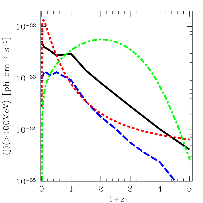
Figure 1.— Comoving volume-average emissivity as a function of redshift for IC emission from structure shocks (solid), $\pi^{0}$-decay and associated e^± IC emission (long-dash), LDDE blazar model (short-dash), PLE blazar model (long-short-dash).

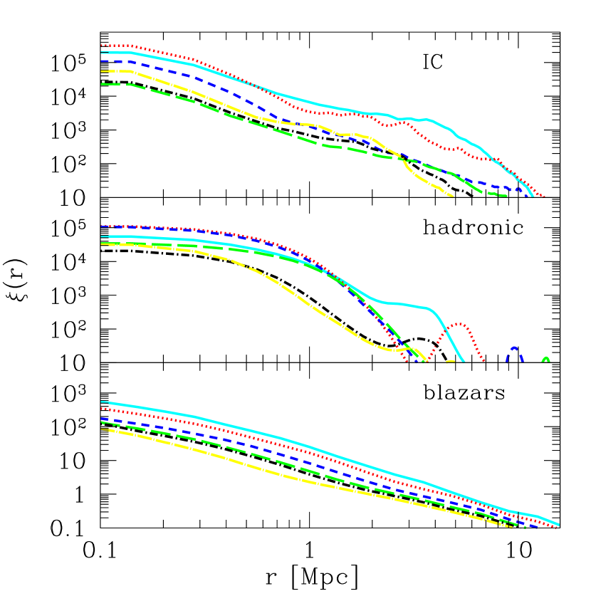
Figure 2.— Spatial correlation function. Solid, dot, short-dash, long-dash, dot-short-dash and dot-long-dash indicate, respectively, redshift $z$=$0.01,0.1,0.5,1,2,3$ for IC emission from structure shocks (top), $z$=$0,0.1,0.5,1,2,3$ for hadronic emission (middle) and $z$=$0.1,0.4,1,1.6,2,3$ (bottom) for blazars.

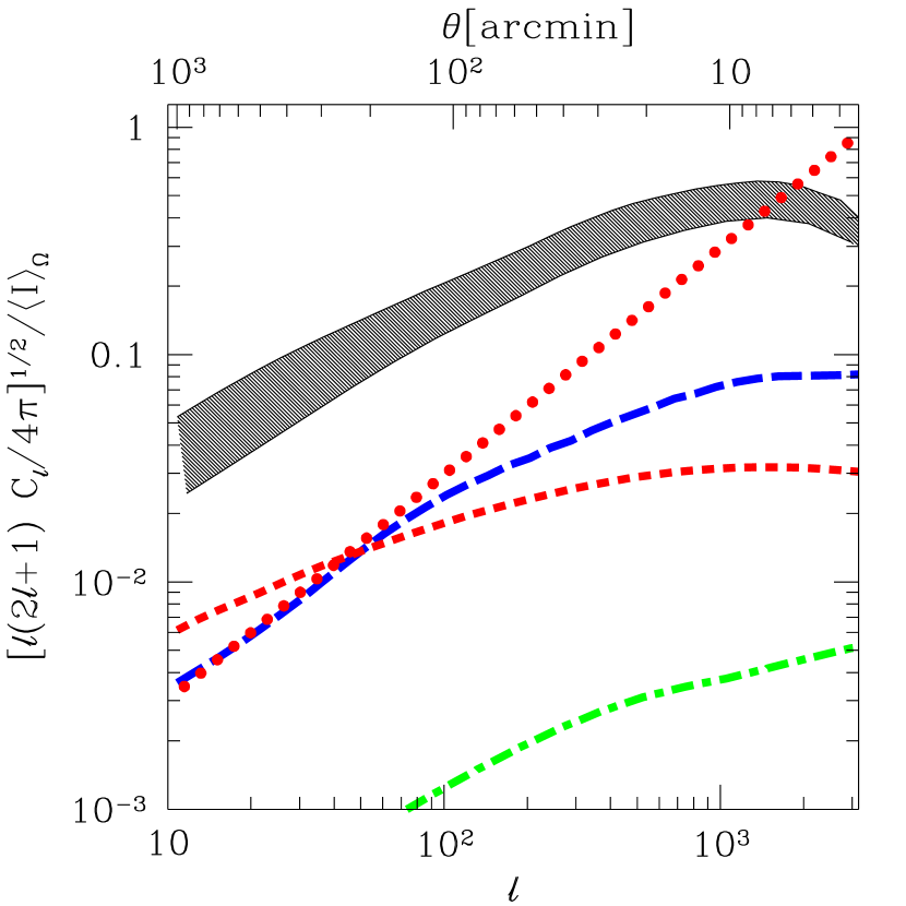
Figure 3.— Power spectrum of angular correlation function for: $\gamma$-ray emission from IC at structure shocks (shaded area), hadronic processes in cluster cores (long-dash), LDDE blazar model (short-dash) and PLE blazar model (short-long-dash) and Poisson noise from unresolved blazars (dot).

References

- Ando & Komatsu (2006) Ando, S., & Komatsu, E. 2006, Phys. Rev. D73, 023521
- Ando et al. (2006a) Ando, S., et al., 2006a, MNRAS, (astro-ph/0610155)
- Ando et al. (2006b) —. 2006b, PRD, (astro-ph/0612467)
- Bell (1978) Bell, A. R. 1978, MNRAS, 182, 147
- Bennett (1990) Bennett, K. 1990, Nucl. Phys. B, 14B, 23
- Chiang & Mukherjee (1998) Chiang, J., & Mukherjee, R. 1998, ApJ, 496, 752
- Colafrancesco & Blasi (1998) Colafrancesco, S., & Blasi, P. 1998, Astropart. Phys. , 9, 227
- Cuoco et al. (2006) Cuoco, A., et al. 2006, (astro-ph/0612559)
- Di Matteo et al. (2004) Di Matteo, T., Ciardi, B., & Miniati, F. 2004, MNRAS, 355, 1053
- Fichtel et al. (1975) Fichtel, C. E., et al. 1975, ApJ, 198, 163
- Hasinger et al. (2005) Hasinger, G., Miyaji, T., & Schmidt, M., 2005, A&A, 441, 417
- Kang & Jones (1995) Kang, H., & Jones, T. W. 1995, ApJ, 447, 994
- Keshet et al. (2004) Keshet, U., Waxman, E., & Loeb, A. 2004, JCAP, 04, 006
- Limber (1953) Limber, D. 1953, ApJ, 119, 665
- Loeb & Waxman (2000) Loeb, A., & Waxman, E. 2000, Nature, 405, 156
- Miniati (2001) Miniati, F. 2001, Comp. Phys. Comm. , 141, 17
- Miniati (2002) —. 2002, MNRAS, 337, 199
- Miniati (2003) —. 2003, MNRAS, 342, 1009
- Miniati et al. (2001) Miniati, F., Ryu, D., Kang, H., & Jones, T. W. 2001, ApJ, 559, 59
- Miniati et al. (2000) Miniati, F., et al. 2000, ApJ, 542, 608
- Mücke & Pohl (2000) Mücke, A., & Pohl, M. 2000, MNRAS, 312, 177
- Narumoto & Totani (2006) Narumoto, T., & Totani, T. 2006, ApJ, 643, 81
- Padovani et al. (1993) Padovani, P., et al. 1993, MNRAS, 260, L21
- Pavlidou & Brian (2002) Pavlidou, V., & Brian, B. D. 2002, ApJ, 575, L5
- Peebles (1993) Peebles, P. J. E. 1993, Principles of Physical Cosmology (Princeton New Jersey: Princeton University Press)
- Ryu et al. (1993) Ryu, D., Ostriker, J. P., Kang, H., & Cen, R. 1993, ApJ, 414, 1
- Ryu et al. (2003) Ryu, D., et al., 2003, ApJ, 593, 599
- Spergel et al. (2003) Spergel et al., D. N. 2003, ApJS, 148, 175
- Sreekumar et al. (1998) Sreekumar, P., et al. 1998, ApJ, 494, 523
- Stecker & Salamon (1996) Stecker, F. W., & Salamon, M. H. 1996, ApJ, 464, 600
- Strong et al. (2004) Strong, A. W., et al. 2004, ApJ, 613, 956
- Tegmark & Efstathiou (1996) Tegmark, M., & Efstathiou, G. 1996, MNRAS, 281, 1297
- Thompson et al. (2007) Thompson, T. A., et al. 2007, ApJ, 654, 219
- Waxman & Loeb (2000) Waxman, E., & Loeb, A. 2000, ApJ, 545, L11
- Zhang & Beacom (2004) Zhang, P., & Beacom, J. F. 2004, ApJ, 614, 37