Is the dependence of spectral index on luminosity real in optically selected AGN samples?

Abstract

We critically examine the dependence of spectral index on luminosity in optically selected AGN samples. An analysis of optically selected high-redshift quasars showed an anti-correlation of $\alpha_{OX}$, the spectral index between the rest-frame 2500 Å and 2 keV, with optical luminosity (Miyaji et al. 2006). We examine this relationship by means of Monte Carlo simulations and conclude that a constant $\alpha_{OX}$ independent of optical luminosity is still consistent with this high-z sample. We further find that that contributions of large dispersions and narrow range of optical luminosity are most important for the apparent, yet artificial, $\alpha_{OX}-l_{o}$ correlation reported. We also examine another, but more complete low-z optical selected AGN sub-sample from Steffen et al. (2006), and our analysis shows that a constant $\alpha_{OX}$ independent of optical luminosity is also consistent with the data. By comparing X-ray and optical luminosity functions, we find that a luminosity independent $\alpha_{OX}$ is in fact more preferred than the luminosity dependent $\alpha_{OX}$ model. We also discuss the selection effects caused by flux limits, which might systematically bias the $l_{x}-l_{o}$ relation and cause discrepancy in optically selected and X-ray selected AGN samples. To correctly establish a dependence of $\alpha_{OX}$ of AGNs on their luminosity, a larger and more complete sample is needed and consequences of luminosity dispersions and selection effects in flux limited samples must be taken into account properly.

1 Introduction

The dependence of the spectral index $\alpha_{OX}$ of active galactic nuclei (AGN) on redshift and luminosity has important astrophysical implications on AGN evolution and thus has been studied for many years (e.g. Avni $\&$ Tananbaum 1982; Wilkes et al. 1994; Green et al. 1995; Bechtold et al. 2003; Vignali et al. 2003a; Strateva et al. 2005; Steffen et al. 2006; Hopkins et al. 2007; Kelly et al. 2007). $\alpha_{OX}$ is defined as

$$\alpha_{OX}=\frac{\log(f_{2\ \rm keV}/f_{2500\ \rm\AA})}{\log(\nu_{2\ \rm keV}/\nu_{2500\ \rm\AA})},$$ (1)

where $f_{2\ \rm keV}$ and $f_{2500\ \rm\AA}$ are the rest-frame flux densities at 2 keV and 2500 $\rm\AA$, respectively. Dependence of $\alpha_{OX}$ on redshift means evolution of the accretion process in cosmic time. Most studies have concluded that there is no evidence for a dependence of $\alpha_{OX}$ on redshift (e.g. Avni $\&$ Tananbaum 1982; Strateva et al. 2005), although some studies found that $\alpha_{OX}$ is correlated with redshift (Bechtold et al. 2003; Kelley et al. 2007). Dependence of $\alpha_{OX}$ on luminosity means a non-linear relationship between X-ray and optical luminosity ($L_{X}\propto L_{O}^{e}$, $e\neq 1$), which provides insight into the radiation mechanism. An anti-correlation between $\alpha_{OX}$ and the optical luminosity has been found by many authors in optically selected AGNs with follow-up X-ray measurements at some different epoch, which means that these AGNs span a larger range in optical luminosity than in X-ray luminosity (e.g. Vignali et al. 2003a; Strateva et al. 2005; Miyaji et al. 2006, hereafter M06; Steffen et al. 2006, hereafter S06). Meanwhile, whether $\alpha_{OX}$ depends on luminosity in X-ray selected AGN samples remains unknown (Hasinger 2004; Frank et al. 2007).

As pointed out by Yuan et al. (1998), one of the problems in such studies is that an apparent, yet artificial correlation between $\alpha_{OX}$ and optical luminosity can be caused by dispersions in the optical luminosity. In section 2, we present analysis of the relationship between $\alpha_{OX}$ and optical/X-ray luminosity using data presented in M06, in which we find that dispersions in luminosity can be entirely responsible for the claimed dependence. We also discuss the determining factor for this behavior.

Another problem is the degeneracy between redshift and luminosity in flux-limited samples, where redshift and luminosity are strongly correlated. In section 3, we examine a sub-sample from S06 containing 187 AGNs, which more completely fills the redshift and optical luminosity plane and thus is less affected by such degeneracy. In section 4, we compare the optical quasar luminosity function from Richards et al. (2006) with X-ray quasar luminosity function from Barger et al. (2005) in different $\alpha_{OX}$ models. In section 5, we discuss the selection effects in flux limited samples and the consequently discrepancy in optically selected and X-ray selected samples. Discussion and conclusions are presented in section 6.

We mostly use the logarithms of luminosities and denote them as $l_{x}=\log L_{2\ \rm keV}$ and $l_{o}=\log L_{2500}$, then $\alpha_{OX}=0.3838(l_{x}-l_{o})$, where $L_{2\ \rm keV}$ is the 2 keV monochromatic luminosity and $L_{2500}$ is the 2500 $\rm\AA$ monochromatic luminosity in units of erg s^-1 Hz^-1. We adopt the currently favored cosmology model with $H_{0}$=70 km s^-1 Mpc^-1, $\Omega_{M}=0.3$, and $\Omega_{\Lambda}=0.7$ (e.g. Spergel et al. 2007).

2 Analysis of Miyaji et al. (2006) Sample

2.1 Data Analysis

The sample we use in this section is consisted of 61 high-redshift ($z>2.9$) quasars in Figure 2 of M06 (Miyaji et al. 2006; Vignali et al. 2003b, 2005), excluding the three quasars from archival $\it Chandra$ data in Table 3 in M06 which might be biased toward higher X-ray fluxes. Only six of them have no X-ray detection. M06 found a correlation of $\alpha_{OX}$ with optical luminosity for this high-z sample, while they kept the discussion on the $l_{o}-\alpha_{OX}$ relation open because of possible optical selection effects for variable AGNs which preferentially pick up the optically brighter phases.

To illustrate how dispersions produce artificial correlations in this sample, we carry out two independent analysis. The first one is linear regression of $\alpha_{OX}$, $l_{o}$ and $l_{x}$ in observed data. Without further description, we perform linear regression using methods as follows throughout the paper:

1. For the $\alpha_{OX}-l_{o}$ correlation, we use the EM algorithm in ASURV (Isobe, Feigelson, & Nelson 1986) to derive linear regression parameters, including X-ray undetected quasars;

2. The EM linear regression algorithm in ASURV is based on the traditional ordinary least-squares method which minimizes the residuals of the dependent variable (OLS(Y$\mid$X)). However, for $l_{x}-l_{o}$ correlation, both variables are observed and a different result can be obtained if residuals of the independent variable are instead minimized (e.g. S06). Following S06, we perform linear regression with ASURV using EM algorithm, treating $l_{x}$ as the dependent variables (ILS(Y$\mid$X)) and treating $l_{o}$ as the dependent variables (ILS(X$\mid$Y)), then use the equations given by Isobe et al. (1990) to calculate the bisector of the two regression lines.

3. For the $\alpha_{OX}-l_{x}$, where both independent and dependent variables are upper limits, only Schmitt’s binned method in ASURV is available which may suffer from several drawbacks (Sadler et al. 1989). Hence we abandon upper limit points in $\alpha_{OX}-l_{x}$ plane and only use X-ray detected quasars to derive linear regression parameters.

Spearman correlation coefficients are calculated using ASURV including X-ray undetected quasars. Observational data together with linear regression slopes and Spearman correlation coefficients for $\alpha_{OX}-l_{o}$, $l_{x}-l_{o}$ and $\alpha_{OX}-l_{x}$ correlations are shown in Figure 1. Conflicting correlations arise due to dispersions in luminosity: $\alpha_{OX}=-0.18l_{o}+const$ as shown in solid line in Panel (a), but $\alpha_{OX}=0.20l_{x}+const$ as shown in solid line Panel (c). Therefore the same data produce two totally different results: $l_{x}=0.53l_{o}+const$ or $l_{x}=2.08l_{o}+const$, i.e. $e<1$ or $e>1$ if $L_{X}\propto L_{O}^{e}$. Therefore, depending upon how the regression is done, the conclusion on the relationship between the optical and X-ray luminosities can be significantly different. As shown in Panel (b), the slope of the $l_{x}-l_{o}$ relation does depend on which luminosity is used as the dependent variable. When treating $l_{x}$ as the dependent variable, the slope is $0.54\pm 0.14$ (the flatter dashed line), while it changes dramatically to $2.08\pm 0.45$ (the steeper dashed line) when treating $l_{o}$ as the dependent variable. Using ILS bisector, we find the slope to be $1.05\pm 0.20$ (solid line), which is consistent with $e=1$ (dotted line).

Figure 1: 61 high-redshift quasars in Miyaji et al. (2006). Circles indicate X-ray detected quasars, while arrows indicate upper limits. Panel (a) $\alpha_{OX}$ dependence on the rest frame 2500 $\rm\AA$ monochromatic luminosity. The solid line indicates linear regression results from the EM Algorithm in ASURV. Panel (b) rest frame 2 keV monochromatic luminosity against 2500 $\rm\AA$ one. The solid line indicates the ILS bisector result, and dashed lines indicate ILS(Y$\mid$X) and ILS(X$\mid$Y) results from the EM Algorithm in ASURV, respectively. The $e=1$ relation is shown by dotted line for comparison. Panel (c) $\alpha_{OX}$ dependence on the rest frame 2 keV monochromatic luminosity. The solid line indicates linear regression result using X-ray detected quasars. Spearman correlation coefficients and slopes of fitting lines are indicated in the upper right panel.

The second part of analysis is done with Monte Carlo simulations. Following Yuan et al. (1998), we assume intrinsic optical and X-ray luminosities $\bar{l}_{o}$ and $\bar{l}_{x}$ with a constant mean $\bar{\alpha}_{OX}$,

$$\bar{l}_{x}=\bar{l}_{o}+\bar{\alpha}_{OX}/0.3838,$$ (2)

and $\bar{\alpha}_{OX}=-1.728$ is given by the mean of observed $0.3838(l_{x}-l_{o})$ using the Kaplan-Meier estimator in ASURV, including the six quasars with upper limits. The above relationship is plotted as dotted line in Panel (b) of Figure 1. The observed optical and X-ray luminosities are assumed to be the intrinsic luminosities modified by independent Gaussian dispersions

$$l_{o}=\bar{l}_{o}+\delta l_{o},l_{x}=\bar{l}_{x}+\delta l_{x}=\bar{l}_{o}+\bar{\alpha}_{OX}/0.3838+\delta l_{x},$$ (3)

where $\delta l_{o}$ and $\delta l_{x}$ are Gaussian distributed dispersions with standard deviations $\sigma_{o}$ and $\sigma_{x}$ respectively. Thus, the distribution of $\alpha_{OX}$ is Gaussian with standard deviation

$$\sigma_{\alpha_{OX}}=0.3838(\sigma_{o}^{2}+\sigma_{x}^{2})^{1/2},$$ (4)

where $\sigma_{\alpha_{OX}}=0.154$ is the standard deviation around the linear relationship of Equation (2) for this sample, using 55 X-ray detected AGNs. The ratio of the standard deviations of the optical to the X-ray luminosity dispersion is defined as

$$R_{\sigma}=\frac{\sigma_{o}}{\sigma_{x}}.$$ (5)

In the following we make Monte Carlo simulations by considering 21 values of $R_{\sigma}$ from 0.1 to 10, sampled evenly on a logarithmic scale. We use the observed optical luminosity as $\bar{l}_{o}$ and keep redshift unchanged. Then $l_{o}$, $l_{x}$ and fluxes can be determined using Equations (3)-(5). The X-ray flux limit is determined as follows. Quasars in this sample are from different observations and thus not uniformly sampled. All quasars with $z\leq 3.5$ are X-ray detected. In the range of $z>3.5$, six quasars are not X-ray detected. Five of them, i.e. SDSS 1737+5828, PSS 1435+3057, SDSS 1532-0039, PSS 1506+5220 and PSS 2344+0342 were observed by Chandra with exposure times from 2.61-5.1 ks; SDSS 0338+0021 was observed by XMM-Newton with exposure time 5.49 ks. PSS 1506+5220 has one count in 0.5-2 keV, and all the other five have zero counts. All the other detected sources have counts larger than 1. The average rest-frame $f_{2\ \rm keV}$ flux for one count in 0.5-2 keV of the six quasars is $0.8\times 10^{-32}$ erg cm^-2 s^-1 Hz^-1. So we simply put a flux limit of $f_{2\ \rm keV,\ upper}=1.5\times 0.8\times 10^{-32}$ erg cm^-2 s^-1 Hz^-1. We assume that simulated quasars with $z>3.5$ and $f_{2\ keV}$ less than $f_{2\ \rm keV,\ upper}$ will not be detected: quasars with $0\leq f_{2\ \rm keV}<0.5f_{2\ \rm keV,\ upper}$ will be assigned zero count, and quasars with $0.5f_{2\ \rm keV,\ upper}\leq f_{2\ \rm keV}<1.5f_{2\ \rm keV,\ upper}$ will be assigned 1 count. Then the upper limits of non-detected quasars are at the 95% confidence level and will be calculated according to Kraft et al. (1991), assuming one count corresponds to a flux of $0.8\times 10^{-32}$ erg cm^-2 s^-1.

Then we simulate 100 samples for each of 21 different $R_{\sigma}$ values. For each $R_{\sigma}$, we compute the average slopes and Spearman correlation coefficients $\rho_{sp}$ from the 100 simulated samples and display the results in Figures 2 and 3. Parameters for simulated samples are calculated in the same way as for panels (a) and (c) in Figure 1. As discussed in Strateva et al. (2005), the measurement errors and variability effects bring $\sigma_{x}\sim 0.23$ and $\sigma_{o}\sim 0.17$, and $\sqrt{\sigma_{x}^{2}+\sigma_{o}^{2}}\sim 0.29$. The observed dispersion is 0.4 for the M06 sample and around $0.35-0.4$ for other samples. The extra dispersions could be assigned to either $\sigma_{x}$ or $\sigma_{o}$ as unknown dispersions, so the possible range of $R_{\sigma}$ should be $0.5\sim 1.4$, i.e. $\log(R_{\sigma})\sim-0.3-0.15$. In the range of $\log(R_{\sigma})\sim-0.2-0$, $\rho_{sp}$ and slopes in simulated samples for both $\alpha_{OX}-l_{x}$ and $\alpha_{OX}-l_{o}$ correlations are consistent with observed values within 1.5$\sigma$, as shown in Figures 2 and 3.

Figure 2: Spearman rank correlation coefficients $\rho_{sp}$ as a measure of the $\alpha_{OX}-l_{o}$ and $\alpha_{OX}-l_{x}$ correlation for Miyaji’s sample and simulated samples. Open squares: $\alpha_{OX}-l_{x}$ in simulated samples; solid circles: $\alpha_{OX}-l_{o}$ in simulated samples; upper dashed line: $\alpha_{OX}-l_{x}$ of true data; lower dashed line: $\alpha_{OX}-l_{o}$ of true data; solid line indicates no correlation.

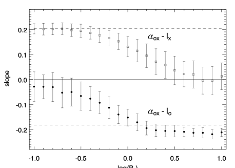
Figure 3: Slopes of the $\alpha_{OX}-l_{o}$ and $\alpha_{OX}-l_{x}$ correlation for Miyaji’s sample and simulated samples. Symbols and lines are as in Figure 2.

From the above two analyses, we conclude that a constant $\alpha_{OX}$ which does not depend on optical luminosity is still consistent with data in this high-z sample.

2.2 Determining factor for an artificial correlation caused by luminosity dispersions

Yuan et al. (1998) pointed out that a dispersion larger for the optical luminosity than for the X-ray luminosity tends to result in apparent, yet artificial correlation of $\alpha_{OX}-l_{o}$. To quantitatively examine the effect of dispersions on the artificial correlation, we make a simple analytic calculation as follows.

As shown in Figure 4, assuming $l_{x}=l_{o}+\rm const.$, dispersions in $l_{x}$ and $l_{o}$ are $\sigma_{x}$ and $\sigma_{o}$, respectively, and the span range of $l_{o}$ is $\Delta l_{o}$. Then locations of AGNs in the $\alpha_{OX}-l_{o}$ plane with average $l_{x}$ and $1\sigma$ range of $l_{o}$ are indicated by the dotted lines in the lower panel, where an apparent correlation appears. We only consider the simplest situation:

1. AGNs are evenly distributed along $l_{o}$ (A concentration around a central $l_{o}$ is equivalent to a smaller $\Delta l_{o}$);

2. AGNs are only distributed $0.3838f\sigma_{o}$ away from $\bar{\alpha}_{OX}$, i.e. $\alpha_{OX}=\bar{\alpha}_{OX}\pm 0.3838f\sigma_{o}$, where $f$ is an unknown positive coefficient to be determined. We will discuss the value of $f$ later.

Then we fit the observed AGNs in the $\alpha_{OX}-l_{o}$ plane, assuming a least chi-squared fitting procedure with same weight in $l_{o}$ and $\sigma_{o}$ (i.e. $\alpha_{OX}/0.3838$) as

$$\chi^{2}=[\sum_{i}((l_{o}(i)-\hat{l}_{o}(i))^{2}+(\alpha_{OX}(i)-\hat{\alpha}_{OX}(i))^{2}/0.3838^{2})]/\sigma_{C}^{2},$$ (6)

where the $l_{o}(i)$ and $\alpha_{OX}(i)$ are observed values, $\hat{l}_{o}(i)$ and $\hat{\alpha}_{OX}(i)$ are the values in the fitting line (indicated by a long solid line with a negative slope in the lower panel of Figure 4) with the least $(l_{o}(i)-\hat{l}_{o}(i))^{2}+(\alpha_{OX}(i)-\hat{\alpha}_{OX}(i))^{2}/0.3838^{2}$, and $\sigma_{C}$ is the typical constant error of $l_{o}$. Then

$$\chi^{2}=\frac{k^{2}}{3(1+k^{2})}(\frac{\Delta l_{o}^{3}}{4}+3\Delta l_{o}(f\sigma_{o})^{2}(1+\frac{1}{k})^{2})/\sigma_{C}^{2},$$ (7)

where $k$ is the slope of the fitting line. The best fit slope $k$ can be derived by solving

$$\frac{d\chi^{2}}{dk}=0,\frac{d^{2}\chi^{2}}{dk^{2}}>0.$$ (8)

The solution is

$$k_{f}=\frac{\Delta l_{o}^{2}}{24f^{2}\sigma_{o}^{2}}-\sqrt{(\frac{\Delta l_{o}^{2}}{24f^{2}\sigma_{o}^{2}})^{2}+1}\\$$ (9)

$$\simeq-12(\frac{f\sigma_{o}}{\Delta l_{o}})^{2}.$$ (10)

The deviation of the approximation in Equation (10) from Equation (9) is less than $20\%$ when $\frac{24f^{2}\sigma_{o}^{2}}{\Delta l_{o}^{2}}<1$. Considering two sub-samples with the same weight and different slopes $k_{1}$ and $k_{2}$ respectively, the slope of combined sample including all points in each sub-samples would be $k_{c}=\tan((\arctan(k_{1})+\arctan(k_{2}))/2)\simeq(k_{1}+k_{2})/2$, where the last $\simeq$ is valid only if $k_{1}\ll 1$ and $k_{2}\ll 1$. Therefore, we can derive the slope of the combined sample considering different $f$ values with different weights by an integration

$$k=\int_{0}^{\infty}k_{f}p(f)df,$$ (11)

where $p(f)$ is the probability of $f$.

Then we take the distribution of $f$ into account. If $\sigma_{x}=0$, and $\sigma_{o}$ follows Gaussian distribution, the probability of $f$ would be

$$p(f)=\sqrt{\frac{2}{\pi}}e^{-\frac{f^{2}}{2}},\ f\geq 0.$$ (12)

Then

$$k\simeq\int_{0}^{\infty}-12(\frac{f\sigma_{o}}{\Delta l_{o}})^{2}\sqrt{\frac{2}{\pi}}e^{-\frac{f^{2}}{2}}df=-6(\frac{\sigma_{o}}{\Delta l_{o}})^{2}$$ (13)

$$\simeq\frac{\Delta l_{o}^{2}}{12\sigma_{o}^{2}}-\sqrt{(\frac{\Delta l_{o}^{2}}{12\sigma_{o}^{2}})^{2}+1}.$$ (14)

Equation (13) shows that the slope of the artificial $\alpha_{OX}-l_{o}$ correlation is directly proportional to $\sigma_{o}^{2}/\Delta l_{o}^{2}$. The significance of the correlation, which could be measured by Spearman correlation coefficient, is always positively correlated to the slope value in the artificial $\alpha_{OX}-l_{o}$ correlation, as shown in Figures 2-3. Therefore, the result in Equation (13) also means the significance of the artificial $\alpha_{OX}-l_{o}$ correlation is proportional to $\sigma_{o}^{2}/\Delta l_{o}^{2}$.

For the M06 sample, $\Delta l_{o}\sim 1.7$ and $\sigma_{o}\sim 0.40$ when $\sigma_{x}=0$, then $k\sim-0.3$. Such estimation of an artificial slope using Equations (13) or (14) is qualitatively consistent with the slope in the $e=1$ simulations, where the value is $k\sim-0.18$ as shown in Figure 3. A reason for the discrepancy is that the absolute slope value is not $\ll 1$, therefore approximations used in our estimation are deviated from true values. Another possible reason, i.e. different fitting procedure used in simulations and our estimation, would more or less contribute to the lower absolute slope values in simulations. In simulations, a linear regression method, which only takes residuals of the dependent variable into account, is used, thus always leading to a lower absolute slope value than methods considering residuals in both variables as used in Equation (7), as shown in Panel (b) in Figure 1.

Figure 4: Schematic sketches for the $l_{x}-l_{o}$ and $\alpha_{OX}-l_{o}$ relationship. Here $l_{x}=l_{o}+\bar{\alpha}_{OX}/0.3838$ and $\bar{\alpha}_{OX}=-1.4$. See section 2.2 for details.

We now discuss consequences of non-zero $\sigma_{x}$. When $\sigma_{x}>0$, the distribution of $f$ will be extended. As shown in Figure 4, point B becomes a distribution in the range of CD within $1\sigma$. When calculating the $\chi^{2}$ of a linear regression with slope $-k$, the contribution of the broadening in B is equivalent to an extension along the $l_{o}$ axis. For example, as shown in Figure 4, the contribution of point C is equivalent to point C’ which has the same $\alpha_{OX}$ as B but smaller $l_{o}$. Therefore, a non-zero $\sigma_{x}$ tends to smooth the distribution of $l_{o}$ and extend its range. When $\sigma_{x}/k$ is comparable with $l_{o}$, it will extend the range of $l_{o}$ significantly. To show this effect, we do another simulation. Based on the M06 sample with a given $\sigma_{o}=0.3$, we calculate the Spearman correlation coefficients and slope for $\alpha_{OX}-l_{o}$ correlation with different $\sigma_{x}$, while other conditions are set to be the same as simulations in section 2.1. As shown in Figure 5, when $\log(\sigma_{x}/\sigma_{o})>0$, i.e. $\sigma_{x}>0.3$ and $\sigma_{x}/k>1.7\sim\Delta l_{o}$, both the Spearman correlation coefficient and the slope tend to move toward zero when $\sigma_{x}$ increases. When $\log(\sigma_{x}/\sigma_{o})>0.5$, i.e. $\sigma_{x}>0.9$ and $\sigma_{x}/k>5.3\sim 3\Delta l_{o}$, there is no correlation in $\alpha_{OX}-l_{o}$ within $1\sigma$. However, as discussed in Section 2.1, even if all extra dispersion in $\alpha_{OX}$ comes from $l_{x}$, $\sigma_{x}$ is unlikely to exceed 0.4 and $\log(\sigma_{x}/\sigma_{o})$ is unlikely to exceed $0.3$.

The effects of $\sigma_{o}$ on the relationship of $\alpha_{OX}-l_{x}$ is similar with the effects of $\sigma_{x}$ on the relationship of $\alpha_{OX}-l_{o}$. Thus we do not need to repeat the above analysis. Moreover, a similar effect as presented here for the $\alpha_{OX}-l_{o}$ correlation would also affect any correlation with a dependent variable $B$, which is not directly observed but derived from $B\propto A^{-1}$, where $A$ is the independent variable, such as the Baldwin effect, which has also been pointed out by Yuan et al. (1998)

In summary, the significance of artificial correlation in $\alpha_{OX}-l_{o}$ is approximately proportional to $\sigma_{o}^{2}/\Delta l_{o}^{2}$, and decreases when $\sigma_{x}$ increases and becomes comparable with $k\Delta l_{o}$, where $k$ is the absolute value of the artificial slope and $\Delta l_{o}$ is the range $l_{o}$ span.

Figure 5: Spearman rank correlation coefficients $\rho_{sp}$ and best-fit slopes of the $\alpha_{OX}-l_{o}$ correlation for simulated samples for various $\sigma_{x}$, with constant $\sigma_{o}=0.3$ and $\bar{\alpha}_{OX}=-1.729$. $l_{o}$ and redshift distributions are from Miyaji et al. (2006).

3 Data Analysis of a sub-sample of AGNs from Steffen et al. (2006)

Another problem in the study of $\alpha_{OX}-l_{o}$ relationship is the degeneracy between redshift and luminosity in flux-limited samples. S06 used a much larger sample than M06 with $\Delta l_{o}\sim 5$, which suppresses the false slope artifacts discussed in section 2. The observed change in $\alpha_{OX}$ across this larger baseline $\Delta l_{o}$ in their sample is sufficiently large that $\alpha_{OX}$ must depend on luminosity, or redshift, or both. To distinguish between luminosity dependence and redshift dependence, first, S06 performed partial correlation analysis using Kendall’s generalized partial $\tau$ to quantitatively show the correlation significance of $\alpha_{OX}-l_{o}$ and $\alpha_{OX}-z$. They found a 13.6$\sigma$ correlation of $\alpha_{OX}-l_{o}$ when controlling $z$, and a 1.3$\sigma$ correlation of $\alpha_{OX}-z$ when controlling $l_{o}$. However, Kelley et al. (2007) has showed that interpretation of Kendall’s $\tau$ is problematic, and Kendall’s $\tau$ for the $\alpha_{OX}-z$ correlation is not necessarily expected to be non-zero when $\alpha_{OX}$ is correlated with $z$. Based on simulations, Kelley et al. (2007) pointed out that the lack of evidence for a significant correlation between $\alpha_{OX}$ and $z$ based on Kendall’s $\tau$ in Steffen et al. (2006) may be the result of an incorrect assumption about the distribution of $\tau$ under the null hypothesis. In spite of most previous studies, Kelley et al. (2007) found that $\alpha_{OX}$ is correlated with both $l_{o}$ and $z$. Moreover, in the partial correlation analysis of $\alpha_{OX}-l_{o}$, consequences of luminosity dispersions, as discussed in section 2, were not taken into account. To show this effect, we select AGNs in three redshift bins, with each bin containing 38 sources, to control the redshift. Then we examine the $\alpha_{OX}-l_{o}$ and $\alpha_{OX}-l_{x}$ relations in each bin, as shown in Figures 6 and 7. Similar to Figure 1, in each redshift bin, $\alpha_{OX}$ is anti-correlated with $l_{o}$, but positively correlated with $l_{x}$, which is caused by luminosity dispersions. Because dispersions always strengthen the anti-correlation of $\alpha_{OX}-l_{o}$, dependence of $\alpha_{OX}$ on $l_{o}$ might be biased toward higher significance by luminosity dispersions, whereas the dependence on $z$ does not suffer such bias.

Second, S06 compared $\alpha_{OX}$ residuals as a linear function of $l_{o}$ and $z$. As shown in their Figure 8, there are systematic residuals of $\alpha_{OX}-\alpha_{OX}(z)$, which indicate that $\alpha_{OX}$ cannot be linearly dependent on redshift alone. However, spectral index might depend on redshift in a non-linear form, as shown in Figure 12 of Strateva et al. (2005). Moreover, it is also possible that $\alpha_{OX}$ depends on both $l_{o}$ and $z$, as shown in Kelley et al. (2007). Using different parameteric models for the redshift and optical luminosity dependencies, Kelley et al. (2007) found the model that is best supported by their data has a linear dependence of $\alpha_{OX}$ on cosmic time, and a quadratic dependence of $\alpha_{OX}$ on $l_{o}$ (the definition of $\alpha_{OX}$ in Kelley et al. (2007) is different from our definition with an opposite sign). Since $l_{o}$ and $z$ are coupled together in flux limited samples, different parameteric models will lead to different results and their best model results depend on the form of the models. In summary, dependence of $\alpha_{OX}$ on $z$, though with lower significance in partial correlation analysis, could not be excluded in S06 sample.

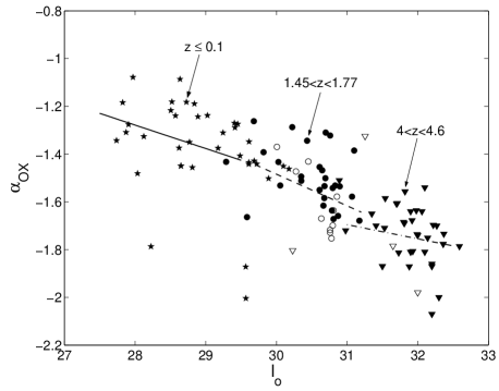
Figure 6: $\alpha_{OX}$ dependece on the rest frame 2500 Å monochromatic luminosity for AGNs in three redshift bins in S06 sample: $z\leq 0.1$ (stars), $1.45<z<1.77$ (circles) and $4<z<4.6$ (downward-pointing triangles). X-ray detected AGNs are represented using filled symbols while upper limits are represented using open symbols. The solid line, dashed line and dash-dotted line indicate linear regression results from the EM Algorithm in ASURV for $z\leq 0.1$, $1.45<z<1.77$ and $4<z<4.6$ samples, respectively.

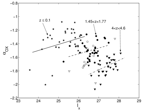
Figure 7: $\alpha_{OX}$ dependece on the rest frame 2 keV monochromatic luminosity for AGNs in three redshift bins in S06 sample: $z\leq 0.1$ (stars), $1.45<z<1.77$ (circles) and $4<z<4.6$ (downward-pointing triangles). X-ray detected AGNs are represented using filled symbols while upper limits are represented using open symbols. The solid line, dashed line and dash-dotted line indicate linear regression results using X-ray detected sources for $z\leq 0.1$, $1.45<z<1.77$ and $4<z<4.6$ samples, respectively.

To avoid possible bias from $\alpha_{OX}-z$ correlation, here we examine a sub-sample from S06 containing 187 AGNs, as shown in the dotted-line box in Figure 3 in S06 (Steffen et al. 2006; Strateva et al. 2005; Vignali et al. 2005; Shemmer et al. 2005; Kelly et al. 2005), which more completely fills the redshift and optical luminosity plane and thus is less affected by such bias. We refer this sample as the ‘low-z sub-sample’. We perform linear regressions in the same procedure as described in section 2.1. Figure 8 presents our results for this sample. Similar to the M06 sample, the low-z sub-sample show conflicting correlations due to dispersions in luminosity: $\alpha_{OX}=-0.16l_{o}+const$ as shown in solid line in Panel (a), but $\alpha_{OX}=0.11l_{x}+const$ as shown in solid line Panel (c). Therefore the same data produce two totally different results: $l_{x}=0.58l_{o}+const$ or $l_{x}=1.40l_{o}+const$, i.e. $e<1$ or $e>1$ if $L_{X}\propto L_{O}^{e}$. As shown in Panel (b), the slope of the $l_{x}-l_{o}$ relation also depends on which luminosity is used as the dependent variable. When treating $l_{x}$ as the dependent variable, the slope is $0.59\pm 0.06$ (the flatter dashed line), while it changes dramatically to $1.45\pm 0.12$ (the steeper dashed line) when treating $l_{o}$ as the dependent variable. Using ILS bisector, we find the slope to be $0.93\pm 0.08$ (solid line), which is consistent with $e=1$ (dotted line). In panel (c), the fit looks different from the trend by eye (bisector fit). As discussed in section 2, when using traditional ordinary least-squared method which minimizes the residuals of the dependent variable, the fit tends to be flatter than the bisector one where residuals of both dependent and independent variables are taken into account. When data points are concentrated at the center, as in Figure 8(c), inconsistence of the two fits becomes large.

Figure 8: 187 low-redshift AGNs from Steffen et al. (2006). Circles indicate X-ray detected AGNs, while arrows indicate upper limits. Panel (a) $\alpha_{OX}$ dependence on the rest frame 2500 $\rm\AA$ monochromatic luminosity. The solid line indicates linear regression results from the EM Algorithm in ASURV. Panel (b) rest frame 2 keV monochromatic luminosity against 2500 $\rm\AA$ one. The solid line indicates the ILS bisector result, and dashed lines indicate ILS(Y$\mid$X) and ILS(X$\mid$Y) results from the EM Algorithm in ASURV, respectively. The $e=1$ relation is shown by dotted line for comparison. Panel (c) $\alpha_{OX}$ dependence on the rest frame 2 keV monochromatic luminosity. The solid line indicates linear regression result using X-ray detected quasars. Spearman correlation coefficients and slopes of fitting lines are indicated in the upper right panel.

Interestingly, but not surprisingly, results of ILS$(\alpha_{OX}\mid l_{o})$ are consistent with results of ILS$(l_{x}\mid l_{o})$, and results of ILS$(\alpha_{OX}\mid l_{x})$ are consistent with results of ILS$(l_{o}\mid l_{x})$, as shown in Table 1 and Figures 1 and 8. The reason is that artificial correlations seen in $\alpha_{OX}-l_{o}$ relation, i.e. $0.3838(l_{x}-l_{o})-l_{o}$ relation, corresponds to least-squares method which minimizes the residuals of $l_{x}$, which is the same as in $l_{x}-l_{o}$ relation, and thus leads to a slope less than the true one where residuals of both variables are considered. Such results indicate that for $l_{x}-l_{o}$ relation, regression results based on the traditional ordinary least-squares method which minimizes residuals of the dependent variable suffer from effects caused by luminosity dispersion and are thus not reliable. Instead, weighting both $l_{o}$ and $l_{x}$ in the regression, i.e. ILS bisector, would be a more robust methodology. Moreover, the degree to which the slopes of ILS$(\alpha_{OX}\mid l_{x})$ and ILS$(\alpha_{OX}\mid l_{o})$ are inconsistent indicates the degree of artificial correlation discussed in section 2. When the slopes converge to the same value, the artificial correlation would be suppressed.

Table 1: Slopes of $l_{x}-l_{o}$ relation in M06 and low-z sub-sample derived from different regression methods.

Regression method	M06	low-z sub-sample
ILS$(\alpha_{OX}\mid l_{o})$	0.53 $\pm$ 0.13	0.58 $\pm$ 0.05
ILS$(l_{x}\mid l_{o})$	0.54 $\pm$ 0.14	0.59 $\pm$ 0.06
ILS$(\alpha_{OX}\mid l_{x})$	2.08 $\pm$ 0.48	1.40 $\pm$ 0.10
ILS$(l_{o}\mid l_{x})$	2.08 $\pm$ 0.45	1.45 $\pm$ 0.12

We conclude for this sample that a constant $\alpha_{OX}$ which does not depend on luminosity is also consistent with data.

4 Comparison of Optical and X-ray Luminosity Functions

For a complete sample of broad line AGN including optical and X-ray observations (detections or upper limits), slopes in optical and X-ray quasar luminosity functions (LFs) should be the same after correct transformations. When converting optical luminosity to X-ray luminosity, different $\alpha_{OX}$ models would lead to different X-ray LF shapes in the optical frame. Thus we can test whether a particular $\alpha_{OX}$ model is correct by comparing the two LFs. We use the optical quasar LF from Richards et al. (2006) and AGN hard X-ray LF from Barger et al. (2005).

We investigate the following two $\alpha_{OX}$ models:

1. a constant $\alpha_{OX}$, $l_{x}=l_{o}-3.92$;

2. $\alpha_{OX}$ from Steffen et al. (2006), $l_{x}=0.72l_{o}+4.53$;

We follow Hopkins, Richards & Hernquist (2007) to calculate the binned LFs. For each $\alpha_{OX}$ model, an overall normalization factor is applied in the X-ray LF to get the minimum $\chi^{2}$, which means that we are comparing just the slopes of LFs. Results are presented in Figure 9. A constant $\alpha_{OX}$ which does not depend on luminosity (left panels) is consistent with data, and is more preferred than the $\alpha_{OX}$ models given by S06 (right panels).

However, from this comparison we cannot reach a strong conclusion that luminosity dependent $\alpha_{OX}$ is excluded completely, for three reasons as follows. First, there are very few data points here in the X-ray LF. Second, as pointed out by Richards et al. (2005), such comparison is not strictly quantitative since X-ray selected samples and optically selected samples are not identical. Moreover, the bright-end slopes from different X-ray samples are different (Barger et al. 2005; Ueda et al. 2003; Hasinger, Miyaji, & Schmidt 2005). Hopkins, Richards & Hernquist (2007) combined a large set of LF measurements and took obscuration and scattering into account, and in their analysis the luminosity functions can be reconciled reasonably well with the $\alpha_{OX}$ model in S06. However, since the constraints on the present bright-end X-ray LFs are poor, the fact that the LFs could be reconciled reasonably well with S06 in their work probably just reflects the large X-ray error bars.

Figure 9: Comparison of the SDSS DR3 optical quasar luminosity function from Richards et al. (2006) (lines with errorbars) with AGN hard X-ray luminosity function from Barger et al. (2005) (crosses with errorbars). Left panels show the LFs with $e=1$ (luminosity independent spectral index). Right panels show the results with $e=0.72$ (spectral index is anti-correlated with luminosity). Different rows show results at different redshift range. For each panel, an overall normalization factor is applied in X-ray LF to get the minimum $\chi^{2}$.

5 Selection effects in flux limited samples: optically selected samples vs X-ray selected samples

In this section, we discuss the selection effects in flux limited samples. For a given AGN luminosity function, assuming the observed optical and X-ray luminosities are the intrinsic values modified by dispersions which might be caused by variabilities or observational errors, there are three possibilities in a flux limited sample:

a) lower fraction of more luminous AGNs are missed;

b) higher fraction of more luminous AGNs are missed;

c) same fractions of more luminous and fainter AGNs are missed, so the relationship between $l_{x}-l_{o}$ remains unchanged.

Assuming the slope of $l_{x}-l_{o}$ relation (without further description, slope=$e$ in $l_{x}=e\times l_{o}+const$ throughout this section) is unity, and at a certain redshift the number density of AGN decreases with luminosity, Figure 10 shows schematic sketches for the first two cases in optically selected AGN samples. The upper panels are for case (a), where the density contour lines in luminosity functions in the $l_{o}-z$ plane (each line corresponds to a given constant AGN number density as a function of redshift) are steeper than the flux limits, hence lower fraction of more optical luminous AGNs are missed, and then the slope is biased toward more than unity. The bottom panels are for case (b), where the density contour lines in luminosity functions in the $l_{o}-z$ plane are flatter than the flux limits, hence higher fraction of more optical luminous AGNs are missed, and then the slope is biased toward less than unity. The left panels show flux limits (dashed lines) in $l_{o}-z$ plane, compared with the density contour lines in luminosity functions (solid lines). The left panels show observed AGNs (solid circles) which are above the flux limits (dashed lines), and missed AGNs (open circles) which are below the flux limits, in $l_{o}-l_{x}$ plane. Slope$=1$ are indicated by solid lines.

Figure 10: Schematic sketches for selection effects in optically selected AGN samples. The upper panels are for case (a) and the bottom panels are for case (b). The left panels show flux limits (dashed lines) in $l_{o}-z$ plane, compared with the density contour lines in luminosity functions (solid lines). The left panels show observed AGNs (solid circles) which are above the flux limits (dashed lines), and missed AGNs (open circles) which are below the flux limits, in $l_{o}-l_{x}$ plane. Slope is defined as in $l_{x}=$ slope$\times l_{o}+const$. Slope$=1$ are indicated by solid lines. Note that in the upper-right panel slope$>1$ for detected AGNs, and in the lower-right panel slope$<1$ for detected AGNs, since $l_{x}$ is the x-axis and $l_{o}$ is the y-axis. These sketches, much simplified and only qualitatively correct, are shown for illustration only.

The density contour lines in real luminosity functions are much more complicated than shown in Figure 10, and the real slopes of density contour lines depend on redshifts and luminosities. Moreover, since the fraction of missed AGNs depends on the dispersions of luminosities around the linear relationship of $l_{x}-l_{o}$, the biases also depends on the dispersions. To test whether the slope of $l_{x}-l_{o}$ relation could be biased by flux limits in realistic optically selected AGN samples, we carry out Monte Carlo simulations. We use optical analytical luminosity function from Richards et al. (2005) for $z<3$ AGNs, and Richards et al. (2006) for $z>3$ AGNs. We simulate three optically selected sub-samples, in order to mimic the SDSS, COMBO-17 and high-z samples in S06:

1) a shallow $z<3$ sub-sample with $m_{g}<19$ containing about 155 AGNs, which is similar to the SDSS sample in S06;

2) a deeper $z<3$ sub-sample with $m_{g}<21$ containing about 52 AGNs, which is similar to the COMBO-17 sample in S06;

3) a $4<z<6$ sub-sample with $m_{g}<20$ containing about 55 AGNs, which is similar to the high-z sample in S06.

We do not try to mimic the nearby Seyfert 1 and BQS samples in S06 which are located in $z<0.4$, since the LF in this redshift range has larger errors due to smaller volume. For the two $z<3$ sub-samples, a detection efficiency factor is taken from Figure 6 in Richards et al. (2006). For the $z>4$ sub-sample, a constant detection efficiency is used according to Richards et al. (2006). To show the effects of luminosity dispersions in optically selected flux limited samples, assuming the slope of $l_{x}-l_{o}$ equals unity with dispersions, 1000 simulations, each containing the above three sub-samples, are carried out for each of the following five dispersion models:

1. $\sigma_{o}=0.42$, $\sigma_{x}=0$;

2. $\sigma_{o}=\sigma_{x}=0.3$ for $z<3$ AGNs, $\sigma_{o}=\sigma_{x}=0.5$ for $z>4$ AGNs;

3. $\sigma_{o}=\sigma_{x}=0.3$

4. $\sigma_{o}=\sigma_{x}=0.5$

5. $\sigma_{o}=0$, $\sigma_{x}=0.42$.

where $\sigma_{o}$ and $\sigma_{x}$ are defined as in section 2.1. Models (i) and (v) are extreme cases, in order to show the bias direction when $\sigma_{o}$ or $\sigma_{x}$ is dominating. Models (ii) $\sim$ (iv) can show the effects of dispersion, and dispersion evolution in cosmic time.

The Monte Carlo analysis was performed by generating a combined sample containing the above three sub-samples for each of the five dispersion models as follows: first, the redshift and luminosity ranges are divided into grids with $\delta z=0.1$ and $\delta M_{g}=0.3$, then the detection probability in a given grid is proportional to $dV(z)\times\Phi(z,M_{g})\times\eta$, where $dV(z)$ is the volume element in comoving space, $\Phi(z,M_{g})$ is the luminosity function, and $\eta$ is the detection efficiency. In a given grid, AGNs are randomly produced following an uniform distribution, and the total number of AGNs in the grid is determined by a poisson process with expectation $\bar{N}(z,M_{g})=dV(z)\times\Phi(z,M_{g})\times\eta\times C$, where C is a constant for a given sub-sample with given luminosity dispersions, adjusted to make the average number of detected AGNs to be 155, 52 and 55 for the three sub-samples, respectively. The conversion from $M_{g}$ to the intrinsic optical luminosity $\bar{l}_{o}$ follows Richards et al. (2005), and the intrinsic X-ray luminosity $\bar{l}_{x}=\bar{l}_{o}-4$. Second, luminosity dispersions are applied, where the observed $l_{o}$ and $l_{x}$ are drawn from the Gaussian distribution around $\bar{l}_{o}$ and $\bar{l}_{x}$ with given dispersions $\sigma_{o}$ and $\sigma_{x}$, respectively. Third, flux limits are applied, AGNs with $m_{g}>$ flux limit are detected. The above procedure select about 262 AGNs for each dispersion model, where about 155 in sub-sample 1), 52 in sub-sample 2) and 55 in sub-sample 3). Then the above procedure is repeated 1000 times to get 1000 independent samples.

The slope in each simulated sample is calculated using FITEXY (Press et al. 1992) assuming the same error in $l_{o}$ and $l_{x}$. The distributions of slopes in simulated optically selected flux limited samples are shown in Figure 11. The relative probabilities are normalized with peak values equal unity. From left to right are the five dispersion models (i) to (v) respectively. The mean values $\pm$ standard deviations of slopes in simulations of the five models are: $0.76\pm 0.05,\ 0.89\pm 0.06,\ 0.97\pm 0.05,\ 1.04\pm 0.11,$ and $1.23\pm 0.06$, respectively. In models (iii) and (iv), $\sigma_{o}=\sigma_{x}=0.3$ and 0.5, flux limited simulations are consistent with the assumed slope$=1$, i.e. the slopes are not biased. However, when $\sigma_{o}\neq\sigma_{x}$ or $\sigma_{o},\ \sigma_{x}$ change in cosmic time, slopes in flux limited simulations might be biased, as shown in models (i), (ii) and (v). Slopes in model (i), i.e. $0.76\pm 0.05$, is consistent with the slope in S06, i.e. $0.72\pm 0.01$. However, since $\sigma_{o}=0.42$ and $\sigma_{x}=0$ is an unrealistic extreme case, this does not mean that the non-unity slope of $l_{x}-l_{o}$ relation is totally caused by such selection effects. Note that slope values in Figures 11 depend on the selection method, i.e. flux limits and number of AGNs in each sub-sample, hence another different optical samples will have different results.

Figure 11: The distributions of slopes in simulated optically selected flux limited samples, where $l_{x}=$slope$\times l_{o}+$constant. The relative probabilities are normalized with peak values equal unity. ¿From left to right are the five dispersion models (i) to (v) listed in the text, respectively.

We do not simulate X-ray selected flux limited samples for two reasons. First, if the slope of $l_{o}-l_{x}$ equals unity, X-ray AGNs are identical to optical AGNs, and the X-ray LF will be the same as optical LF with $l_{x}=l_{o}+$ constant, as suggested in section 4. Therefore, the results here can be applied to X-ray selected sample with similar flux limits after switching $\sigma_{o}$ and $\sigma_{x}$. Second, X-ray LFs have larger errors than optical LFs due to smaller samples. Therefore, it is our purpose to just point out the fact that the slope will be biased in flux limited X-ray samples, rather than focusing on a particular X-ray selected sample.

While a number of previous studies of optical selected AGNs have reported that $\alpha_{OX}$ is anti-correlated with luminosity (e.g. Strateva et al. 2005; Steffen et al. 2006), whether $\alpha_{OX}$ depends on luminosity in X-ray selected AGN samples remains unknown. Hasinger (2004) found no $\alpha_{OX}$ dependence on either luminosity or redshift in soft X-ray selected samples. Frank et al. (2007) found in their Chandra Deep Field-North sample $l_{x}=(0.808\pm 0.047)l_{o}+const.$. They also found the slope decreases when only brighter sources are included, and the slope increases when only fainter sources are included. It is possible that the slope might be biased in this flux limited sample and the magnitude of biases are different when using different flux limit. As shown in Figure 11, if $\sigma_{o}>\sigma_{x}$, an optically selected sample like in S06 will be biased toward a flatter slope. Moreover, if the X-ray LF is similar to optical LF and the X-ray sample is consisted of AGNs with similar flux limits, the X-ray sample will be biased toward a steeper slope. Therefore, even if optically selected AGNs and X-ray selected AGNs are identical, the slope in the optically selected sample will be flatter than the slope in the X-ray selected sample, which can properly explain the observed discrepancy.

In summary, selection effects in flux limited samples might bias the $l_{o}-l_{x}$ relation and cause discrepancy in the $l_{o}-l_{x}$ relation in optically selected samples and X-ray selected samples, especially when $\sigma_{o}\neq\sigma_{x}$ or $\sigma_{o},\ \sigma_{x}$ change in cosmic time. The magnitude of the bias and discrepancy depend on the luminosity function, flux limits of the sample, and dispersions in optical and X-ray luminosities. Note that even if such selection effects do bias the slope of the $l_{o}-l_{x}$ relation toward the observed discrepancy between optical and X-ray samples, it is not necessarily the only reason. It is possible that optically selected samples and X-ray selected samples are consisted of different AGNs, so slopes of the $l_{o}-l_{x}$ relation in optically selected samples will be different from slopes in X-ray selected ones. As discussed in Brusa et al. (2007), about $40\%$ of the X-ray selected AGNs in their COSMOS sample would have not been easily selected as AGN candidates on the basis of purely optical criteria, either because similar colors to dwarf stars or field galaxies, or because they are not point like sources in morphological classification. Moreover, optically selected AGNs and X-ray selected AGNs might be typically in different evolution stages and thus are not identical (Shen et al. 2007).

6 Discussion and Conclusions

In summary, we have investigated the correlation between the spectral index $\alpha_{OX}$ and optical/X-ray luminosities in AGNs by means of linear regressions, Monte Carlo simulations, simplified analytic estimations and comparison of X-ray and optical luminosity functions. We have reached five conclusions:

1. The dependence of $\alpha_{OX}$ on optical luminosity found in Miyaji et al. (2006) may not be an underlying physical property. It remains unknown whether $e<1$ or $e>1$ if $L_{X}\propto L_{O}^{e}$ in this high-z sample.

2. The luminosity dependence can be artificially generated very easily by luminosity dispersions. The significance of artificial correlation in $\alpha_{OX}-l_{o}$ is approximately proportional to $\sigma_{o}^{2}/\Delta l_{o}^{2}$, where $\sigma_{o}$ is the optical luminosity dispersion and $\Delta l_{o}$ is the range that $l_{o}$ spans, and decreases when $\sigma_{x}$ increases and becomes comparable with $k\Delta l_{o}$, where $k$ is the absolute value of the artificial slope. This effect also affects the Baldwin effect. Instead of regressions only weighting one variable, weighting both $l_{o}$ and $l_{x}$, i.e. ILS bisector, in the regression would be a more robust methodology to avoid such bias.

3. In a more complete low-z sub-sample from Steffen et al. (2006), $\alpha_{OX}$ must depend on luminosity, or redshift, or both. However, a luminosity independent $\alpha_{OX}$ is still consistent with data. Redshift dependencies cannot be ruled out and may be large, but somewhat hidden because of luminosity dispersions, which generate artificial luminosity correlations in each redshift bin.

4. In the comparison of X-ray (Barger et al. 2005) and optical quasar (Richards et al. 2006) LFs, a luminosity independent $\alpha_{OX}$ is consistent with data, and more preferred than the luminosity dependent $\alpha_{OX}$ model given by S06.

5. Selection effects in flux limited samples might bias the $l_{o}-l_{x}$ relation and cause discrepancy in the $l_{o}-l_{x}$ relation in optically selected sample and X-ray selected sample, especially when $\sigma_{o}\neq\sigma_{x}$ or $\sigma_{o},\ \sigma_{x}$ change in cosmic time. The magnitude of the bias depends on the luminosity function, flux limits of the sample, and dispersions in optical and X-ray luminosities.

It therefore remains inconclusive whether the anti-correlation between AGN spectral index and optical luminosity is true. Even if $\alpha_{OX}$ does depend on optical luminosity, the currently adopted slope value might be biased and deviate from the intrinsic value. To correctly establish a dependence of $\alpha_{OX}$ of AGNs on their luminosity, a larger and more complete sample, such as from multi-wavelength surveys, is needed and consequences of luminosity dispersions and selection effects in flux limited samples must be taken into account properly.

References

- (1) Anvi, Y., & Tananbaum, H. 1982, ApJ, 262, L17
- (2) Brusa, M., et al. 2007, ApJS, accepted (astro-ph/0612358)
- (3) Barger, A. J., et al. 2005, AJ, 129, 578
- (4) Bechtold, J., et al. 2003, ApJ, 588, 119
- (5) Frank, S., Osmer, P., & Mathur, S. 2007, ApJ, submitted (astro-ph/0612352)
- (6) Green, P. J., et al. 1995, ApJ, 450, 51
- (7) Hasinger, G., 2004, in Merloni A., Nayakshin S., Sunyaev R., eds, Growing Black Holes: Accretion in a Cosmological Context. Springer-Verlag, Berlin (astro-ph/0412576)
- (8) Hasinger, G., Miyaji, T., & Schmidt, M. 2005, A&A, 441, 417
- (9) Hopkins, P. F., Richards, G. T., & Hernquist, L. 2007, ApJ, submitted (astro-ph/0605678)
- (10) Isobe, T., Feigelson, E. D., & Nelson, P. I. 1986, ApJ, 306, 490
- (11) Isobe, T., Feigelson, E. D., Akritas, M. G., & Babu, C. J. 1990, ApJ, 364, 104
- (12) Kelly, B. C., et al. 2005, Memorie della Societa Astronomica Italiana, 76, 87
- (13) Kelly, B. C., et al. 2007, ApJ, accepted (astro-ph/0611120)
- (14) Kraft, R. P., Burrows, D. N., & Nousek, J. A. 1991, ApJ, 374, 344
- (15) Miyaji, T., Hasinger, G., Lehmann, I., & Schneider, D. P. 2006, AJ, 131, 659 (M06)
- (16) Press, W. H., et al. 1992, Numerical Recipes in FORTRAN (Second ed.; Cambridge: Cambridge Univ. press)
- (17) Richards, G. T., et al. 2006, AJ, 131, 2766
- (18) Richards, G. T., et al. 2005, MNRAS, 360, 839
- (19) Sadler, E. M., Jenkins, C. R., & Kotanyi, C. G. 1989, MNRAS, 240, 591
- (20) Shemmer, O., et al. 2005, ApJ, 630, 729
- (21) Shen, Y., et al. 2007, ApJ, 654, L115
- (22) Spergel, D. N., et al. 2007, ApJ, submitted (astro-ph/0603449)
- (23) Steffen, A. T., et al. 2006, AJ, 131, 2826 (S06)
- (24) Strateva, I. V., et al. 2005, AJ, 130, 387
- (25) Ueda, Y., et al. 2003, ApJ, 598, 886
- (26) Vignali, C., Brandt, W. N., & Schneider, D. P. 2003a, AJ, 125, 433
- (27) Vignali, C., et al. 2003b, AJ, 125, 2876
- (28) Vignali, C., Brandt, W. N., Schneider, D. P., & Kaspi, S. 2005, AJ, 129, 2519
- (29) Wilkes, B. J., Tananbaum, H., Worrall, D. M., Avni, Y., Oey, M. S., & Flanagan, J. 1994, ApJS, 92, 53
- (30) Yuan, W., Siebert, J., & Brinkmann, W. 1998, A&A, 334, 498