Asteroseismology: a powerful tool to complement planet transits

Abstract

The study of stellar oscillations - asteroseismology - has revolutionized our understanding of the physical properties of the Sun and similar potential for other stars has been demonstrated in recent years. In particular, asteroseismic studies can constrain the stellar size, temperature and composition, which are important parameters to our understanding of planetary structure and evolution. This makes asteroseismology a very powerful tool to complement planetary transits. As an example, the transit measurement alone does not give the radius of the planet unless the radius of the host star is known, which again requires a known distance to the system. Transit measurements will therefore often require additional measurements to establish the radius of the planet. With asteroseismology we can determine the radius of a star to very high precision (2–3%) using only the photometric transit measurements. This will be very valuable for a mission such as Kepler, which will produce photometric time series of very high quality.

School of Physics, University of Sydney, 2006 NSW, Australia

Institut for Fysik og Astronomi (IFA), Aarhus Universitet, 8000 Aarhus, Denmark

School of Physics, University of Sydney, 2006 NSW, Australia

1. Introduction

Asteroseismology is a very powerful tool. This is because we can measure the frequencies of the stellar oscillations to a very high accuracy, and the oscillations can give us information about the stars that we cannot otherwise measure, helping us to constrain better the stellar parameters. In the last few years we have seen quite a breakthrough in results, which indicates the great potential of asteroseismology as a tool in relation to the search and study of exoplanets. For thorough reviews on asteroseismology see Brown & Gilliland (1994); Christensen-Dalsgaard (2004)

2. Asteroseismology of solar-like stars

In Fig. 1 (left panel) we show the luminosity of the Sun observed as a star for four hours by the VIRGO instrument on board the SOHO spacecraft. The Sun oscillates in many modes simultaneously, each mode with a slightly different frequency, which gives the complex sinusoidal pattern seen in Fig. 1 (left panel).

Figure 1.: Left panel: Luminosity (in parts per million) of the Sun observed as a star by VIRGO (green band) after granulation with time scales longer than $\sim 9\,$minutes has been removed from the data. The cadence is 1 minute. Right panel: Fourier transform of the solar time series similar to that seen in the left panel but including granulation at all time scales (60 days of VIRGO observations).

This is clearly revealed when we take the Fourier transform of the time series (but of longer time span). The square root this transform, also called the amplitude spectrum is shown in Fig. 1 (right panel). Each peak in the amplitude spectrum represents a sinusoidal oscillation and from this we can see that the Sun oscillates in many different modes, with periods of roughly five minutes. The amplitudes of the oscillations are a few parts per million in luminosity, which corresponds to temperature changes of less than 0.01K. The oscillations can also be observed by radial velocity measurements of the surface. The amplitude in velocity is roughly $20\,\mathrm{cm}\,\mathrm{s}^{-1}$, corresponding to a total displacement of the solar surface by about 100 metres. What makes the Sun oscillate in all these modes simultaneously is the convection near the surface. The turbulent gas motion in the convection zone (seen as granulation on the surface) stochastically excites oscillations, which are intrinsically damped, in this broad frequency range. The rising background noise towards lower frequencies seen in Fig. 1 (right panel) is from the random granulation cells themselves. This noise is significantly lower in velocity (see Fig. 3, bottom right).

Each frequency is coming from a mode of a standing sound wave, like in an organ pipe with nodes and anti-nodes, but in three dimensions (see Fig. 2, left panel). Each mode has both a radial part described by the order $n$, which is the number of nodes or spherical ‘shells’, and a surface pattern described by a spherical harmonic. Figure 2 (right panel) shows examples of spherical harmonics of different degree $l$ and order $m$. High-degree modes ($l>3$) cannot be detected when the Sun is observed as a star due to geometric cancellation.

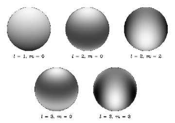
Figure 2.: Left panel: Structure of a single spherical mode with quantum numbers: $n=18$, $l=2$ and $m=2$ (provided by IFA, Aarhus Universitet). Right panel: Spherical harmonics representing the surface behaviour of the oscillations (provided by J. Christensen-Dalsgaard).

The frequency of each mode depends on the sound speed predominantly in that part of the Sun where the particular mode spends most of its time. By observing the frequencies of many modes, the sound speed inside the Sun can be reconstructed. This is extremely interesting because the sound speed depends on physical parameters like temperature, density and composition. For example, hydrogen turns into helium as the Sun gets older and the sound speed and - hence the frequencies - change. Therefore, we can in principle measure the age of the Sun.

A large number of stars are expected to show oscillations that are stochastically driven by convection as in the Sun (also known as solar-like oscillations). Stars located on the cool side of the classical instability strip have convection near the surface, and are therefore expected to show solar-like oscillations. Figure 3 (left panel) shows a Hertzsprung-Russell diagram where different regions of known stellar pulsations are indicated. In recent years solar-like oscillations have been detected in a large range of stars from dwarfs to red giants (indicated in Fig. 3, left panel). These results are mostly based on velocity measurements obtained from the ground (Bedding & Kjeldsen 2006). A few examples of these detections can be seen in Fig. 3 (right panels). The most luminous stars (and biggest) oscillate at the lowest frequencies, which is clearly seen.

Figure 3.: Left panel: Hertzsprung-Russell diagram with names and approximate locations of known groups of pulsating stars. The lower dashed line is the zero age main sequence. The two parallel long dashed lines bracket the instability strip. Stellar evolution tracks (grey curves) are shown for 1, 2, 3, 4 and 7 M_⊙. Stars that have shown evidence of solar-like oscillations are indicated. (The figure is slightly modified compared to the original, which was kindly supplied by J. Christensen-Dalsgaard.) Right panel: Observed power spectra (power=amplitude squared) of the oscillations in the Sun and four other stars. The horizontal axis is the observed frequency in milli Hertz on a logarithmic scale. The power has been normalized to show the same peak height in each plot. The actual amplitudes increase up the plot, and the peak power in $\xi\,$Hya is roughly 30 times that of the Sun. These results are all based on radial velocity measurements. For all but the Sun they are obtained from the ground (Sun (Gabriel et al. 1997); $\alpha\,$Cen A (Butler et al. 2004); $\beta\,$Hyi (Bedding et al. 2001); $\eta\,$Boo (Kjeldsen et al. 1995); $\xi\,$Hya (Frandsen et al. 2002)).

From ground it is extremely difficult to measure the oscillations using photometry due to the Earth’s atmosphere, especially for the less evolved stars, which show the smallest amplitudes. From space, however, detection of oscillations in a true analogue of the Sun is possible.

3. Extracting physical parameters

The seismic signature of solar-like oscillations is a nearly regular spaced comb pattern in the amplitude spectrum. The characteristic spacings in this pattern can be used to characterize the star.

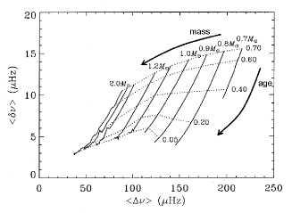
Figure 4.: Left panel: Similar to Fig. 1 but for a shorter frequency range for greater detail. The degree $l$ for each mode is indicated. Right panel: Small versus large separation (in micro Hertz) for stellar evolutionary tracks (solid curves) of different mass. Dotted curves indicate constant central hydrogen abundance. The arrow label age indicates the direction of the stellar evolution for each track. (The figure is a slightly modified version of the original provided by J. Christensen-Dalsgaard.)

In Fig. 4 (left panel) we show in more detail the amplitude spectrum in Fig. 1 (right panel). The degree $l$ for each mode is indicated. We see two characteristic frequency separations: the large separation, which is between modes of the same degree $l$ (but successive radial order $n$, which for the Sun is in the order of 10–30), and the small separations. The large separation ($\Delta\nu$) is a direct measure of the stellar density, while the small separation ($\delta\nu$) is sensitive to the mean molecular weight in the core (hence age) of the star. This is illustrated in Fig. 4 (right panel), which shows stellar evolutionary tracks of different mass (solid curves) in the $\delta\nu$ versus $\Delta\nu$ plane. The dashed lines indicate constant central hydrogen abundance.

4. Constraining the planet radius

A planet transit potentially gives a very precise measure of the radius of the planet relative to its host star (Holman et al., this proceedings). However, additional observations are required to establish the actual size scale. Basically, we cannot tell if it is a transit of a big star by big planet, or a transit of a small star by a small planet. Seismology can be of significant help to constrain the actual stellar radius (and hence the radius of the planet when combined with the transit depth), using only the photometric transit data. The requirements are that the precision is high enough and that the data sample the oscillations. These requirements depend very much on where in the HR diagram the star is located, as both oscillation amplitude and period vary significantly across the HR diagram.

Without applying asteroseismology and without a distance measurement, the stellar radius has to be constrained by spectroscopy and photometry. In this case we can determine the temperature to roughly 100 K (or 2%), and the absolute luminosity to approximately 40%. The accuracy in the radius is therefore roughly 20%. From the stellar location in the HR diagram we can further obtain a mass estimate to about 10% using stellar models.

From seismology we get the large separation to a very high accuracy, at least 0.5% for Kepler targets. Since the mean density of the star is proportional to the large separation squared, this seismic measure gives the density to about 1%. Combining that with the 2% temperature determination reduces the uncertainty in the mass to roughly 5% (in addition to a smaller uncertainty in the luminosity of approximately 10%). This mass estimate together with the seismic density measurement finally provides a 2–3% radius estimate, which is a tremendous improvement.

For Kepler, parallax measurements are expected to be derived at the end of the mission, which will lower the uncertainty in the luminosity to about 2% from the parallaxes alone. This implies a better mass estimate to roughly 3%, and hence a radius estimate of approximately 1% if combined with the seismic measurement of the large separation. This in turn improves the precision of the temperature to less than 1%. In addition, the small separation can be measured to at least 10%, which for a solar mass star implies that the age will be known to better than 1 Gyr.

5. Conclusion

• Including seismology to determine the stellar parameters improves significantly the accuracy with which we can characterize the stars, and hence their planets.

• This can be obtained without complicated and time-consuming calculations of pulsation models for each star.

• Only the data already obtained to detect the transits need to be used, provided the data sampling is high enough. Cadence requirements are about once per minute for a true Sun-like star, and up to roughly half an hour for a giant star.

• This technique would help tremendously for a mission such as Kepler, where the precision in the radius estimates of the host stars are improved by a factor of 7 without any parallax information and by a factor of 20 when parallaxes become available.

In the last few years, the field of asteroseismology has taken advantage of the observational techniques developed in the quest of detecting and studying exoplanets. This has mostly been from ultra-high precision Doppler measurements, but in the coming years very accurate photometry from space will become available. With these observational techniques in common, very similar data sets and complementary but supporting science goals, there is an obvious opportunity for exoplanet research to take advantage of the extremely precise measurements that seismology can offer in order to determine the properties of planet-hosting stars. This makes the future for both research fields very exciting.

Acknowledgments.

This paper has been supported by the Astronomical Society of Australia and by the Australian Research Council. We are grateful for the VIRGO data being publicly available.

References

- Bedding et al. (2001) Bedding, T. R., Butler, R. P., Kjeldsen, H., et al. 2001, ApJ, 549, L105
- Bedding & Kjeldsen (2006) Bedding, T., & Kjeldsen, H. 2006, ESA SP-624: Proceedings of SOHO 18/GONG 2006/HELAS I, Beyond the spherical Sun, 18,
- Brown & Gilliland (1994) Brown, T. M. & Gilliland, R. L. 1994, ARA&A, 32, 37
- Butler et al. (2004) Butler, R. P., Bedding, T. R., Kjeldsen, H., et al. 2004, ApJ, 600, L75
- Christensen-Dalsgaard (2004) Christensen-Dalsgaard, J. 2004, Solar Phys., 220, 137
- Frandsen et al. (2002) Frandsen, S., Carrier, F., Aerts, C., et al. 2002, A&A, 394, L5
- Gabriel et al. (1997) Gabriel, A. H., Charra, J., Grec, G., et al. 1997, Solar Phys., 175, 207
- Kjeldsen et al. (1995) Kjeldsen, H., Bedding, T. R., Viskum, M., & Frandsen, S. 1995, AJ, 109, 1313