The penetration of FUV radiation into molecular clouds

Abstract

Context. FUV radiation strongly affects the physical and chemical state of molecular clouds, from protoplanetary disks to entire galaxies.

Aims. The solution of the FUV radiative transfer equation can be complicated if the most relevant radiative processes such us dust scattering and gas line absorption are included, and have realistic (non–uniform) properties, i.e. if optical properties are depth dependent.

Methods. We have extended the spherical harmonics method to solve for the FUV radiation field in externally or internally illuminated clouds taking into account gas absorption and coherent, nonconservative and anisotropic scattering by dust grains. The new formulation has been implemented in the Meudon PDR code and thus it will be publicly available.

Results. Our formalism allows us to consistently include: $(i)$ varying dust populations and $(ii)$ gas lines in the FUV radiative transfer. The FUV penetration depth rises for increasing dust albedo and anisotropy of the scattered radiation (e.g. when grains grow towards cloud interiors).

Conclusions. Illustrative models of illuminated clouds where only the dust populations are varied confirm earlier predictions for the FUV penetration in diffuse clouds (A_V$<$1). For denser and more embedded sources (A_V$>$1) we show that the FUV radiation field inside the cloud can differ by orders of magnitude depending on the grain properties and growth. Our models reveal significant differences regarding the resulting physical and chemical structures for steep vs. flat extinction curves towards molecular clouds. In particular, we show that the photochemical and thermal gradients can be very different depending on grain growth. Therefore, the assumption of uniform dust properties and averaged extinction curves can be a crude approximation to determine the resulting scattering properties, prevailing chemistry and atomic/molecular abundances in ISM clouds or protoplanetary disks.

1 Introduction

Far–UV (FUV) radiation ($h\nu$ $<$13.6 eV) strongly affects the physical and chemical state of dusty molecular clouds in many evolutionary stages: from star forming regions (Lequeux et al. (1981); Stutzki et al. (1988); Bally et al. (1998)) and protoplanetary disks (Johnstone et al. (1998); Aikawa et al. (2002)), to circumstellar envelopes around evolved stars (Huggins & Glassgold (1982); Habing (1996)) and supernova remnants (Shull & McKee (1979); Chevalier & Fransson (1994)). Thus, the accurate knowledge of the intensity of the FUV radiation field as a function of cloud depth is of crucial importance in a plethora of astrophysical environments. Penetration of FUV radiation strongly depends on dust grains properties through the scattering of photons, but it also depends on the gas properties (chemical composition, density, etc.) through the absorption of hundreds of discret electronic lines from the most abundant species (H, H₂, and CO). This proccess is, in addition, an efficient excitation mechanism for molecular species (Black & van Dishoeck (1987); Sternberg & Dalgarno (1989)). Gas absorption lines reach extremely large opacities and, due to saturation, they can be very broad and fully absorb the FUV continuum.

The so called spherical harmonics method, in which the specific intensity of the FUV radiation field is expanded into series of Legendre polynomials, is an efficient way to solve the plane–parallel radiative transfer equation if gas opacity is neglected and if dust grains have uniform optical properties, e.g. the same extinction cross–section, albedo and scattering phase function (Flannery et al. (1980); Roberge (1983)). Nevertheless, astronomical observations over the full spectral domain show a more complex scenario, where dust grain populations evolve depending on the environmental conditions from polycyclic aromatic hydrocarbons (PAHs) and very small grains (VSGs) to bigger grains (BGs) likely formed by accretion or coagulation (Boulanger et al. (1988); Desert et al. (1990); Joblin et al. (1992); Draine (2003); Dartois (2005)). Also, the average extinction law (e.g., Cardelli, Clayton & Mathis (1989)) is based on observations toward low–extinction line of sights ($A_{V}\lesssim 5$), and it has been questioned by recent observations toward more embedded regions ($A_{V}\geq 15$). A better knowledge of the extinction properties at large A_V is critical. In particular, there is evidence that the reddening curve tends to flatten at high extinction depths (Moore et al. (2005)), consistent with grain growth and dust processing along the line of sight. Therefore, the attenuation of FUV radiation will dramatically depend on the (generally poorly understood) grain composition and optical properties that, of course, are likely to change from source to source according to the interstellar (ISM) and circumstellar (CSM) dust life–cycle. In addition to this dust–shielding, self–shielding through gas line absorption can result in an efficient protection of H₂ and CO, and the starting point of a rich chemistry even in irradiated media such as protoplanetary disks, translucent clouds, starbursts galaxies or, more generally, photodissociation regions (PDRs; see Hollenbach & Tielens (1997) for a review).

The spherical harmonics method also has been implemented to study the radiative transfer and dust extinction in galaxies as a whole by associating the source function with the emissivity of a given distribution of stars through the galaxy (di Bartolomeo et al. (1995); Baes & Dejonghe (2001)). Uniform grain properties and the absence of gas line absorption are assumed. For unidimensional problems, the spherical harmonics method is found to be by far the most efficient way to solve for the radiative transfer equation compared to Monte Carlo or ray tracing techniques (Baes & Dejonghe (2001)).

The detailed information provided by high angular resolution observations (e.g. Gerin et al. (2005); Goicoechea et al. (2006)), revealing fine differences even between similar sources, should be followed by a sophistication in the radiative transfer modeling. Inclusion of gas (discrete line absorption) and varying grain populations (e.g. different extinction curves) as a function of cloud depth requires a modification of the original method (Flannery et al. (1980); Roberge (1983)). In this work we present an extension of the spherical harmonics method for a radiative transfer equation with depth dependent coefficients in plane–parallel geometry. We used this method to solve for the radiation field in illuminated clouds at wavelengths longer than Lyman cut–off at $\sim$912 Å  taking into account gas absorption and scattering by dust grains. The method can also include the source function for embedded emission of photons, and therefore it can explicitly take into account any source of internal radiation.

In Secs. 2 and 3 we present the formulation of the method while in Secs. 4 and 5 we show several astrophysical applications to understand the role of FUV penetration for the photochemistry of molecular clouds. In particular, we present a few examples including H Lyman lines, H₂ electronic transitions within the Lyman and Werner bands and CO electronic transitions together with varying dust properties. The penetration of FUV radiation for the typical conditions prevailing in a diffuse cloud (such us $\zeta$ Ophiuchi) and in higher extinction objects (such as the Orion Bar or a strongly illuminated protoplanetary disk) are discussed.

2 The equation of radiative transfer with variable coefficients

The specific intensity of radiation, $I_{\lambda}(s,\mu)$, in plane-parallel geometry is a solution of the radiative transfer equation:

$$\mu\frac{\partial I_{\lambda}(s,\mu)}{\partial s}=-[\alpha_{\lambda}(s)+\sigma_{\lambda}(s)]\,I_{\lambda}(s,\mu)+\frac{\sigma_{\lambda}(s)}{2}\,\,\int_{-1}^{+1}R_{\lambda}(s,\mu,\mu^{\prime})\,I_{\lambda}(s,\mu^{\prime})\,d\mu^{\prime}+j_{\lambda}(s)$$ (1)

where the spatial scale $s$ and the angle $\theta=cos^{-1}\mu$ are the independent variables and where the dependence of quantities on wavelength $\lambda$ and on $s$ has been explicitly written. In the most general problem, $\alpha_{\lambda}(s)=\alpha_{\lambda}^{g}(s)+\alpha_{\lambda}^{d}(s)$ is the line–plus–continuum absorption coefficient, $\sigma_{\lambda}(s)$ is the dust scattering coefficient, $j_{\lambda}(s)$ is the emission coefficient of any source of internal radiation and $R_{\lambda}(s,\mu,\mu^{\prime})$ is the angular redistribution function (we assume that the radiation field has azimuthal symmetry about normal rays). In this work, the opacity is due to coherent (no energy redistribution in the scattered photons), nonconservative (a fraction of photons are absorbed), anisotropic scattering by dust grains as well as to gas line absorption, that is:

$$d\tau=-(\alpha_{\lambda}+\sigma_{\lambda})\,ds$$ (2)

(note that $\tau$ increases toward the decreasing direction of $s$) and the radiative transfer Eq. (1) gets the more familiar form

$$\mu\frac{\partial I_{\lambda}(\tau,\mu)}{\partial\tau}=I_{\lambda}(\tau,\mu)-\frac{\omega_{\lambda}(\tau)}{2}\,\int_{-1}^{+1}R_{\lambda}(\tau,\mu,\mu^{\prime})\,I_{\lambda}(\tau,\mu^{\prime})\,d\mu^{\prime}-S^{*}_{\lambda}(\tau,\mu)=I_{\lambda}(\tau,\mu)-S_{\lambda}(\tau,\mu)$$ (3)

where $\omega_{\lambda}=\frac{\sigma_{\lambda}}{\alpha_{\lambda}+\sigma_{\lambda}}$ is a new effective albedo (the dust scattering cross–section over the total dust+gas extinction cross–section) which tends to the pure dust albedo for wavelengths free of lines, but tends to 0 (true gas absorption) at the line cores. Intermediate values are found in the line wings. $S^{*}_{\lambda}=\frac{j_{\lambda}}{\alpha_{\lambda}+\sigma_{\lambda}}$ is the source function for the true emission by ”embedded photon sources”. In the following we assume that $S_{\lambda}^{*}$=0. Thus we ignore dust thermal emission (negligible in the FUV for ISM clouds) or any other source of internal illumination. Hence, our source function only corresponds to the external illumination photons scattered by dust grains. However, inclusion of $S_{\lambda}^{*}$ in our method is trivial. The interested reader is refererred to Appendix A.

The cloud extends from $\tau=0$ to $\tau=\tau_{max}$ with a possibility that $\tau_{max}=\infty$. Boundary conditions require $I_{\lambda}(\tau,\mu)$ to match the incident intensity at $\tau=0$ and $\tau=\tau_{max}$. Note the implicit sign convention on $\mu$: $\theta=\pi$ points towards positive values of $\tau$, that is $\mu=-1$ for a ray perpendicular to the cloud and penetrating into it from $\tau=0$ (see Fig. 1). Thus, boundary conditions specify $\chi^{-}(\mu)=I_{\lambda}(0,\mu)$ ($\mu<0$) and $\chi^{+}(\mu)=I_{\lambda}(\tau_{max},\mu)$ ($\mu>0$), where $\chi^{\pm}(\mu)$ are the illuminating radiation fields reaching both cloud surfaces (of course they can be different).

Compared to other works where the spherical harmonics method has been applied to solve for the FUV radiation field (e.g. Flannery et al. (1980); Roberge (1983); di Bartolomeo et al. (1995); Baes & Dejonghe (2001); Le Petit et al. (2006)), the optical properties in the radiative transfer equation (e.g., effective albedo and asymmetry parameter) are wavelength– and cloud depth–dependent for the first time.

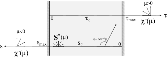
Figure 1: Adopted geometry and sign conventions for a cloud with embedded sources of photons $S^{*}(\mu)$ and illuminated at both surfaces by $\chi^{\pm}(\mu)$.

3 The spherical harmonics method for line and continuum transfer

3.1 The $P_{L}$ approximation

In this method, the angular dependence of the radiation field $I(\tau,\mu)$ is expanded in a truncated series of Legendre polynomials $P_{l}(\mu)$ which form a complete orthogonal set within the range (-1,1) in which $\mu$ varies:

$$I(\tau,\mu)=\sum_{l=0}^{L}(2l+1)\,f_{l}(\tau)\,P_{l}(\mu)$$ (4)

where the dependence on $\lambda$ is no longer shown. In the following sections we show that the mean intensity of the radiation field at each depth point $J(\tau)$ has the simple form $J(\tau)=f_{0}(\tau)$, i.e. the first coefficient of the expansion in Eq. (4), which is often the only quantity needed for the integration of radiation field–dependent physical parameters (e.g. photoionization and photodissociation rates). This is one of the reasons why the method is so attractive. However, a large number of expansion terms has to be used in order to correctly sample the angular dependence of the radiation field, we typically use $L+1=2M=20$ (note that dust scattering can be highly anisotropic at the considered wavelengths).

If the grain scattering phase function $p(\tau,cos\,\Theta)$ only depends on the angle $\Theta$ between the incident and scattered radiation, $R(\tau,\mu,\mu^{\prime})$ can also be expanded (see e.g., Chandrasekhar (1960); Roberge (1983)) as:

$$R(\tau,\mu,\mu^{\prime})=\sum_{l=0}^{L}(2l+1)\,\sigma_{l}(\tau)\,P_{l}(\mu)\,P_{l}(\mu^{\prime})$$ (5)

in terms of the $\sigma_{l}(\tau)$ coefficients of the Legendre expansion of $p(\tau,cos\,\Theta)$:

$$p(\tau,cos\,\Theta)=\sum_{l=0}^{L}(2l+1)\,\sigma_{l}(\tau)\,P_{l}(cos\,\Theta)$$ (6)

The standard model of scattering by interstellar grains (Henyey & Greenstein (1941)) assumes the simple scattering phase function:

$$p(cos\,\Theta)=\frac{1-g^{2}}{(1+g^{2}-2g\,cos\,\Theta)^{3/2}}$$ (7)

which can be also expanded in Legendre polynomials in terms of the ”$g$–asymmetry parameter” ($=<cos\,\Theta>$) i.e., the mean angle of the scattered radiation ($g=1/2\int_{-1}^{+1}\mu\,p(\mu)\,d\mu$, with $\mu=cos\,\Theta$). Here we adopt a $\tau$-dependent Henyey–Greenstein phase function (other phase functions can be used if they can also be expanded). Therefore we write:

$$p(\tau,cos\,\Theta)=\sum_{l=0}^{L}(2l+1)\,g_{l}(\tau)\,P_{l}(cos\,\Theta)$$ (8)

where $g_{l}(\tau)=\sigma_{l}(\tau)$ and $g_{0}(\tau)=1$. Thus, the angular redistribution function $R(\tau,\mu,\mu^{\prime})$ has two obvious limiting cases, $g(\tau)=0$ (isotropic scattering) and $g(\tau)=\pm 1$ with $R(\tau,\mu,\mu^{\prime})=\delta(\mu\mp\mu^{\prime})$ (pure backward or forward scattering).

Substitution of Eqs. (4) and (5) into the transfer equation (3) and using appropriate recurrence formulae leads to the finite ($L+1$) set of coupled, linear, first order differential equations in the unknown $f_{l}(\tau)$ coefficients, with $l=0,...,L$.

$$lf^{\prime}_{l-1}(\tau)+(l+1)f^{\prime}_{l+1}(\tau)=(2l+1)\,[1-\omega(\tau)\sigma_{l}(\tau)]\,f_{l}(\tau)$$ (9)

where $f^{\prime}=\partial f/\partial\tau$. We recall that compared to Roberge (1983) this is not a constant coefficient equation so numerical integration is necessary. In the ”$P_{L}$ approximation” a sufficiently large odd $L$ value has to be chosen to obtain an accurate solution of the problem. The system (9) can be written as:

$$\mathbf{f^{\prime}}(\tau)=\mathbf{A^{-1}\mathnormal{(\tau)\,}f}(\tau)$$ (10)

with:

$$\mathbf{A}(\tau)=\left(\begin{array}[]{cccccc}0&h_{0}^{-1}\\ h_{1}^{-1}&0&2h_{1}^{-1}\\ &2h_{2}^{-1}&0&\ddots\\ &&3h_{3}^{-1}&&(L-1)h_{L-2}^{-1}\\ &&&\ddots&0&Lh_{L-1}^{-1}\\ &&&&Lh_{L}^{-1}&0\end{array}\right)$$ (11)

where:

$$h_{l}(\tau)=(2l+1)\,(1-\omega(\tau)\sigma_{l}(\tau))\hskip 28.45274pt$$ (12)

In summary, we have to solve for a linear boundary value problem with non constant coefficients with the additional difficulty of huge variations of the total opacity within small variations in the wavelength and cloud position grids, e.g. from $\lambda$ in a saturated line center ($\tau_{\lambda}\sim$10⁷) to $\lambda$ in an adjacent (line free) continuum region ($\tau_{\lambda}\sim$10). In the following, we show an extension of the spectral method of Flannery et al. (1980) and Roberge (1983) to solve for the FUV radiative transfer.

3.2 The eigenvalues solution

3.2.1 Numerical solution

The $\mathbf{A}^{-1}(\tau)$ matrix has $L+1=2M$ eigenvalues which are real, non-zero and non-degenerate and which occur in positive-negative pairs, see Appendix A of Roberge (1983). Using a similar notation as Roberge, let $k_{m}(\tau),\,m=\pm 1,\cdots,\pm M$ be the eigenvalues verifying $k_{-m}(\tau)=-k_{m}(\tau)$, and $\mathbf{R(\tau)}$ be the matrix of eigenvectors, that is:

$$\sum_{j}\mathbf{A}^{-1}(\tau)_{lj}\,R_{jm}(\tau)=k_{m}(\tau)\,R_{lm}(\tau)$$ (13)

which also verifies the $R_{l,-m}(\tau)=(-1)^{l}\,R_{lm}(\tau)$ relation. The depth–dependence of the eigenvalues $k_{m}(\tau)$ and eigenvectors $R_{lm}(\tau)$ complicates the solution of the problem compared to the (only dust) problem with uniform optical grain properties. The computation of $k_{m}(\tau)$ and $R_{lm}(\tau)$ is given in Appendix C.

The $\mathbf{R}(\tau)$ matrix of eigenvectors can still be used to define an auxiliary set of variables $\mathbf{y}(\tau)=\mathbf{R^{-1}}(\tau)\,\mathbf{f}(\tau)$, or:

$$f_{l}(\tau)=\sum_{-M}^{-1}R_{lm}(\tau)\,y_{m}(\tau)+\sum_{1}^{M}R_{lm}(\tau)\,y_{m}(\tau)$$ (14)

so that

$$\mathbf{f}^{\prime}=\mathbf{A}^{-1}\,\mathbf{R}\,\mathbf{y}$$ (15)

Therefore, in terms of the new $\mathbf{y}(\tau)$ variables, Eq. (10) can be rewritten as:

$$\mathbf{y^{\prime}}=\mathbf{R}^{-1}\,\mathbf{A}^{-1}\,\mathbf{R}\,\mathbf{y}-\mathbf{R}^{-1}\,\mathbf{R}^{\prime}\,\mathbf{y}=\mathbf{K}\,\mathbf{y}-\mathbf{R}^{-1}\,\mathbf{R}^{\prime}\,\mathbf{y}$$ (16)

To write Eq. (16) we have used the fact that $(\mathbf{R^{-1}A^{-1}R})_{lm}=k_{l}\,\delta_{lm}$ and thus $\mathbf{K}(\tau)$ is a diagonal matrix with the $k_{m}(\tau)$ eigenvalues of $\mathbf{A^{-1}(\tau)}$ on its diagonal. The fact that $\mathbf{R}^{\prime}(\tau)\neq 0$ adds the last matrix term in Eq. (16) due to the depth–dependence of the coefficients. This term is neglected in Le Petit et al. (2006). However, $\mathbf{R}^{\prime}$ is not null neither when the grain optical properties depend on the cloud depth (even if gas is neglected) nor when gas line absorption is included (even if grain properties are uniform). Unfortunately, the system of Eqs. (16) is uncoupled only if the $\mathbf{R}^{-1}\,\mathbf{R}^{\prime}\,y$ term is null (as in Roberge 1983), otherwise more manipulations are required to solve the problem consistently. If we define $\mathbf{Q}=\mathbf{R}^{-1}\mathbf{R}^{\prime}\,\mathbf{y}=-\mathbf{L}\,\mathbf{y}\,$, then Eq. (16) can be simply written as:

$$y^{\prime}_{m}=k_{m}(\tau)\,y_{m}+[\mathbf{L\,y}]_{m}(\tau)$$ (17)

for $m=\pm 1,...,\pm M$. In order to solve this particular problem we turn the system of differential equations (17) into an integral problem. To do that we first introduce the following integral equation:

$$y_{m}(\tau)=e^{a_{m}(\tau)}\left[C_{m}+\int_{\tau_{m}}^{\tau}\,e^{-a_{m}(t)}\,[\mathbf{L\,y}]_{m}(t)\,dt\right]$$ (18)

where $a_{m}(\tau)$ is an arbitrary function so that $a_{m}(\tau_{m})$=0. The system of Eqs. (18) represents a general set of integral equations that verify $y_{m}(\tau_{m})=C_{m}$ (to be found from the boundary conditions). If a given function $y_{m}$ is a solution of the above equation, by taking its derivative with respect to $\tau$ one gets:

$$y^{\prime}_{m}(\tau)=a^{\prime}_{m}(\tau)y_{m}(\tau)+[\mathbf{L\,y}]_{m}(\tau)$$ (19)

which means that $y_{m}$ as defined in Eqs. (18) is also a solution of the original system of differential Eqs. (17) if and only if $a^{\prime}_{m}(\tau)=k_{m}(\tau)$. Therefore, $a_{m}(\tau)=\int_{\tau_{m}}^{\tau}\,k_{m}(t)\,dt$. This demonstration shows that the $k_{m}$ eigenvalues of $\mathbf{A^{-1}}$ (and no others) are the right exponential factors that do attenuate the radiation field, which is consistent with the original problem described by Eqs. (10). In the present work we solve Eqs. (18) with an iterative scheme² and thus compute:

$$y_{m}^{(n+1)}(\tau)=e^{\int_{\tau_{m}}^{\tau}\,k_{m}(t)\,dt}\left[C_{m}^{(n+1)}+\int_{\tau_{m}}^{\tau}\,e^{-\int_{\tau_{m}}^{t}\,k_{m}(t^{\prime})\,dt^{\prime}}\,[\mathbf{L\,y}^{(n)}]_{m}(t)\,dt\right]$$ (20)

by using an appropriate (physical) initial guess for $y_{m}^{(n)}$, where $n$ is the iteration step. This iterative procedure shows that the solution if forced, at any step, by the exponential factor $e^{\int_{\tau_{m}}^{\tau}\,k_{m}(t)\,dt}$ to follow the behavior dictated by the ”true” eigenvalues of the problem (i.e. those of the original coupling matrix $\mathbf{A^{-1}}$) that are known before the iteration procedure is started. In Appendix B we give details on the error bound associated with the iterative scheme and we show that the numerical solution derived for the FUV radiation field correctly satisfies the original system of Eqs. (10).

At each iteration step we have to compute the integration constants $C_{m}$ by a convenient selection of $\tau_{m}$. To ensure that only exponentials with negative arguments appear, it is necessary to set $\tau_{m}=0$ for $m<0$ and $\tau_{m}=\tau_{max}$ for $m>0$. In order to have easier to read equations, we now introduce some convenient notations:

$$E_{m}^{-}(\tau)=\exp\left(\int_{0}^{\tau}k_{m}(t)\,dt\right)\,\,\,(m<0)\,\hskip 28.45274pt{\rm or}\hskip 28.45274pt\,E_{m}^{-}(\tau)=\exp\left(-\int_{0}^{\tau}k_{m}(t)\,dt\right)\,\,\,(m>0)$$ (21)

Note that $E_{-m}^{-}(\tau)=E_{m}^{-}(\tau)$, and $E_{m}^{-}(0)=1$. We also define:

$$E_{m}^{+}(\tau)=\exp\left(\int_{\tau}^{\tau_{max}}k_{m}(t)\,dt\right)\,\,\,(m<0)\,\hskip 28.45274pt{\rm or}\hskip 28.45274pt\,E_{m}^{+}(\tau)=\exp\left(-\int_{\tau}^{\tau_{max}}k_{m}(t)\,dt\right)\,\,\,(m>0)$$ (22)

with $E_{m}^{+}(\tau_{max})=1$ and $E_{m}^{+}(\tau)\times E_{m}^{-}(\tau)=E_{m}^{+}(0)=E_{m}^{-}(\tau_{max})$. Using the above notations, we have:

$$y_{m}(\tau)=E_{m}^{-}(\tau)\,C_{m}-\int_{0}^{\tau}\frac{E_{m}^{-}(\tau)}{E_{m}^{-}(t)}\,q_{m}(t)\,dt\qquad(m<0)$$ (23)

$$y_{m}(\tau)=E_{m}^{+}(\tau)\,C_{m}+\int_{\tau}^{\tau_{max}}\frac{E_{m}^{+}(\tau)}{E_{m}^{+}(t)}\,q_{m}(t)\,dt\qquad(m>0)$$ (24)

Note the change of sign in the second equation due to the inversion of $\int_{\tau_{max}}^{\tau}$. To further simplify these expressions, we define:

$$D_{m}^{-}(\tau)=\int_{0}^{\tau}\frac{E_{m}^{-}(\tau)}{E_{m}^{-}(t)}\,q_{m}(t)\,dt\qquad(m<0)$$ (25)

$$D_{m}^{+}(\tau)=\int_{\tau}^{\tau_{max}}\frac{E_{m}^{+}(\tau)}{E_{m}^{+}(t)}\,q_{m}(t)\,dt\qquad(m>0)$$ (26)

which satisfy $D_{m}^{-}(0)=0$ and $D_{m}^{+}(\tau_{max})=0$. Therefore, the $\mathbf{y}(\tau)$ variables are finally written compactly as:

$$y_{m}(\tau)=E_{m}^{-}(\tau)\,C_{m}-D_{m}^{-}(\tau)\qquad(m<0)$$ (27)

$$y_{m}(\tau)=E_{m}^{+}(\tau)\,C_{m}+D_{m}^{+}(\tau)\qquad(m>0)$$ (28)

and the original $f_{l}(\tau)$ terms in the Legendre expansion of the radiation field $I(\tau,\mu)$ are then given by:

$$f_{l}(\tau)=\sum_{m=-M}^{-1}R_{lm}(\tau)\,\left(C_{m}\,E_{m}^{-}(\tau)-D_{m}^{-}(\tau)\right)+\sum_{m=1}^{M}R_{lm}(\tau)\,\left(C_{m}\,E_{m}^{+}(\tau)+D_{m}^{+}(\tau)\right).$$ (29)

3.2.2 Boundary conditions: Clouds with two sides illumination

We consider a unidimensional plane–parallel cloud of finite size with an external radiation field at both cloud surfaces ($\tau=0$ and $\tau=\tau_{max}$) defined by $\chi^{-}(\mu)$ and $\chi^{+}(\mu)$ respectively (see Fig. 1). From Eq. (29) we have:

$$f_{l}(0)=\sum_{m=-M}^{-1}R_{lm}(0)\,C_{m}+\sum_{m=1}^{M}R_{lm}(0)\,\left(C_{m}\,E_{m}^{+}(0)+D_{m}^{+}(0)\right)$$ (30)

$$f_{l}(\tau_{max})=\sum_{m=-M}^{-1}R_{lm}(\tau_{max})\,\left(C_{m}\,E_{m}^{-}(\tau_{max})-D_{m}^{-}(\tau_{max})\right)+\sum_{m=1}^{M}R_{lm}(\tau_{max})\,C_{m}.$$ (31)

At the $\tau=0$ side, the solution must match, at each $\lambda$, the incoming radiation field with $\mu<0$, i.e. $I(0,\mu)=\chi^{-}(\mu)$, with

$$I(0,\mu)=\sum_{l=0}^{L}(2l+1)\,f_{l}(0)\,P_{l}(\mu)\hskip 56.9055pt{\rm or:}$$ (32)

$$I(0,\mu)=\sum_{m=-M}^{-1}C_{m}\,\sum_{l=0}^{L}(2l+1)\,R_{lm}(0)\,P_{l}(\mu)+\sum_{m=1}^{M}\left(C_{m}\,E_{m}^{+}(0)+D_{m}^{+}(0)\right)\,\sum_{l=0}^{L}(2l+1)\,R_{lm}(0)\,P_{l}(\mu).$$ (33)

At the $\tau=\tau_{max}$ side, the solution must match, at each $\lambda$, the incoming radiation field with $\mu>0$, i.e. $I(\tau_{max},\mu)=\chi^{+}(\mu)$, with:

$$I(\tau_{max},\mu)=\sum_{l=0}^{L}(2l+1)\,f_{l}(\tau_{max})\,P_{l}(\mu)\hskip 56.9055pt{\rm or:}$$ (34)

$$I(\tau_{max},\mu)=\sum_{m=-M}^{-1}\left(C_{m}\,E_{m}^{-}(\tau_{max})-D_{m}^{-}(\tau_{max})\right)\,\sum_{l=0}^{\infty}(2l+1)\,R_{lm}(\tau_{max})\,P_{l}(\mu)+\sum_{m=1}^{M}C_{m}\,\sum_{l=0}^{L}(2l+1)\,R_{lm}(\tau_{max})\,P_{l}(\mu).$$ (35)

Nevertheless, since the order $L$ of the expansions is finite, the boundary conditions $I(0,\mu)=\chi^{-}(\mu)$ and $I(\tau_{max},\mu)=\chi^{+}(\mu)$ can not be satisfied at all $\mu$ angles. In this work we use Marck’s conditions that require $I(0,\mu<0)$ and $I(\tau_{max},\mu>0)$ to match the incident radiation fields at $L+1=2M$ strategic angles $\mu_{i}$ given by $P_{L+1}(\mu_{i})=0$, that is, the roots of the Legendre polynomial of degree $L+1$. Note that in these $\mu_{\pm i}$ ($i=\pm 1,...,\pm M$) angles, the solution of the radiation field $I(\tau,\mu_{i})$ is ”exact”.

To further simplify the boundary conditions relations, we now define:

$$T_{im}(0,\mu_{i})=\sum_{l=0}^{L}(2l+1)\,R_{lm}(0)\,P_{l}(\mu_{i})\quad(\mu_{i}<0)$$ (36)

$$T_{im}(\tau_{max},\mu_{i})=\sum_{l=0}^{L}(2l+1)\,R_{lm}(\tau_{max})\,P_{l}(\mu_{i})\quad(\mu_{i}>0)$$ (37)

which gives:

$$I(0,\mu_{i})=\sum_{m=-M}^{-1}C_{m}\,T_{im}(0,\mu_{i})+\sum_{m=1}^{M}\left(C_{m}\,E_{m}^{+}(0)+D_{m}^{+}(0)\right)\,T_{im}(0,\mu_{i})$$ (38)

$$I(\tau_{max},\mu_{i})=\sum_{m=-M}^{-1}\left(C_{m}\,E_{m}^{-}(\tau_{max})-D_{m}^{-}(\tau_{max})\right)\,T_{im}(\tau_{max},\mu_{i})+\sum_{m=1}^{M}C_{m}\,T_{im}(\tau_{max},\mu_{i})$$ (39)

Therefore, the desired $C_{m}$ constants at each iteration step are solutions of the $2M\times 2M$ linear system ($m=0$ excluded):

$$\sum_{\begin{array}[]{c}m=-M\end{array}}^{M}B_{im}\,C_{m}=H_{i}$$ (40)

with the $B_{im}$ coefficients as define in Table 1, and where

$$H_{i}=\left\{\begin{array}[]{lc}I^{-}(0,\mu_{i})-\sum_{m=1}^{M}D_{m}^{+}(0)\,T_{im}(0,\mu_{i})&\quad(\mu_{i}<0)\\ I^{+}(\tau_{max},\mu_{i})+\sum_{m=-M}^{-1}D_{m}^{-}(\tau_{max})\,T_{im}(\tau_{max},\mu_{i})&\quad(\mu_{i}>0)\end{array}\right.$$ (41)

$B_{im}=$	$m<0$	$m>0$
$\mu_{i}<0$	$T_{im}(0,\mu_{i})$	$T_{im}(0,\mu_{i})\,E_{m}^{+}(0)$
$\mu_{i}>0$	$T_{im}(\tau_{max},\mu_{i})\,E_{m}^{-}(\tau_{max})$	$T_{im}(\tau_{max},\mu_{i})$

Table 1: $B_{im}$ coefficients for the two sides illumination boundary conditions in Eq. (40)

For semi–infinite clouds ($\tau_{max}$=$\infty$) with only one side illumination at $\tau$=0 ($\mu_{i}<0$), boundary conditions have to be modified to take into account the no radiation condition at $\tau$=$\infty$ ($\mu_{i}>0$). It is straightforward to show that the $C_{m}$ constants are then solutions of the same linear system shown in Eq. (40) with the $B_{im}$ coefficients now defined as in Table 2 and:

$$H_{i}=\left\{\begin{array}[]{lc}I^{-}(0,\mu_{i})&\quad(\mu_{i}<0)\\ 0&\quad(\mu_{i}>0)\end{array}\right.$$ (42)

$B_{im}=$	$m<0$	$m>0$
$\mu_{i}<0$	$T_{im}(0,\mu_{i})$	$0$
$\mu_{i}>0$	$0$	$T_{im}(\tau_{max},\mu_{i})$

Table 2: $B_{im}$ coefficients for the one side illumination boundary conditions in Eq. (40)

3.3 Iterative procedure

At very large optical depths (e.g. deep inside the cloud or at the core of saturated lines) the intensity of the radiation field tends to zero. Hence, the simplest way to initiate the iterative process is to set $\mathbf{Q}=\mathbf{R}^{-1}\mathbf{R}^{\prime}\,\mathbf{y}=0$. However, this may be far from the real solution, and more realistic guesses should be tried. In practice, the assumption $\tau\rightarrow\infty$ may be too crude and one can add the effect of the external radiation perpendicular to the cloud that penetrates deepest in the cloud, i.e. attenuated by the smallest eigenvalue $k_{\pm 1}$ (that associated with the radiation field in the $|\mu|\simeq 1$ direction). Thus, we guess a first set of $y_{m}(\tau)$, that we call $y_{m}^{0}(\tau)$, from the linear system:

$$\sum_{m=-M}^{-1}R_{lm}(\tau)\,y_{m}^{0}(\tau)+\sum_{m=1}^{M}R_{lm}(\tau)\,y_{m}^{0}(\tau)=f_{l}^{approx}(\tau)$$ (43)

with

$$f_{0}^{approx}(\tau)=\frac{1}{2}\,I(0,-1)\,\exp[-k_{1}(\tau)\,\tau]+\frac{1}{2}\,I(\tau_{max},1)\,\exp[k_{-1}(\tau)(\tau_{max}-\tau)]$$ (44)

Note that only the $l=0$ terms have to be considered. As noted by Flannery et al. (1980) and Roberge (1983), the presence of dust scattering implies that $|k_{\pm 1}|\neq 1$, i.e. the radiation field attenuation factor at large depths is not simply $e^{-\tau}$ but dominated by the $e^{-k_{1}\tau}$ factor. This conclusion obviously applies for the present case with the difference that $k_{\pm 1}$ is now depth–dependent and includes line absorption. This important result can modify the intensity of the FUV radiation field inside optically thick clouds by orders of magnitude depending on the dust grain optical properties. At lower optical depths (e.g., diffuse clouds), the attenuation factor still contains an important contribution from additional terms ($k_{\pm 2},k_{\pm 3},...$).

Now that we have an educated guess for the $y_{m}(\tau)$ variables, we can estimate the new term in Eq. (16) carrying the depth–dependence of the gas and dust coefficients, i.e. the $\mathbf{Q}=\mathbf{R^{-1}}\,\mathbf{R^{{}^{\prime}}}\,\mathbf{y}$ term. Note that $\mathbf{R}^{-1}\mathbf{R}^{\prime}$ need to be evaluated only once, so numerical cost is limited. However, special care should be taken for the $\mathbf{R}^{\prime}$ derivation. Details of the $\mathbf{R^{-1}}$ inversion and $\mathbf{R}^{\prime}$ derivation are given in Appendix D.

We briefly describe the iterative computation of $\mathbf{Q}$: we start by using $\mathbf{Q^{0}}=\mathbf{R}^{-1}\mathbf{R}^{\prime}\,\mathbf{Y^{0}}$ and then compute a first set of $C_{m}^{0}$ from the boundary conditions. With these first $C_{m}^{0}$ and $\mathbf{Q^{0}}$ variables we can now use the general expression Eq. (20) to compute a new set of $y_{m}(\tau)$ to derive a more refined $\mathbf{Q}$ term, and start this proccess again until some prescribed level of convergence in $\mathbf{Q}$ is reached. Thus, if $n$ is the iteration index, $\mathbf{Q}^{(n+1)}$ is computed from $\mathbf{Q}^{(n+1)}=\mathbf{R}^{-1}\,\mathbf{R}^{\prime}\,\mathbf{Y}^{(n+1)}$ with:

$$y_{m}^{(n+1)}(\tau)=C_{m}^{(n+1)}\,E_{m}^{-}(\tau)-D_{m}^{-(n)}(\tau)\qquad(m<0)$$ (45)

$$y_{m}^{(n+1)}(\tau)=C_{m}^{(n+1)}\,E_{m}^{+}+D_{m}^{+(n)}(\tau)\qquad(m>0)$$ (46)

Those expressions have to be computed at each iteration by numerical integration.

3.4 Mean intensity and FUV photon escape probability

Once we have obtained the full depth and angular description of the intensity of the radiation field $I(\tau,\mu_{i})$ through the $f_{l}(\tau)$ coefficients, we show here the simple form that $J(\tau)$ takes. The angular average of the specific intensity is defined as:

$$J(\tau)=\frac{1}{2}\int_{-1}^{+1}I(\tau,\mu)\,d\mu$$ (47)

From the expansion of $I(\tau,\mu)$ we have:

$$\int_{-1}^{+1}I(\tau,\mu)\,d\mu=\sum_{l}(2l+1)\,f_{l}(\tau)\,\int_{-1}^{+1}P_{l}(\mu)\,d\mu$$ (48)

where the only no null sum corresponds to $\int_{-1}^{+1}P_{0}(\mu)\,d\mu=2$. Therefore, as anticipated in Sec. 3.1, the mean intensity of the radiation field at each wavelength and depth reduces to $J(\tau)=f_{0}(\tau)$, that is:

$$J(\tau)=\sum_{m=-M}^{-1}\left(C_{m}\,E_{m}^{-}(\tau)-D_{m}^{-}(\tau)\right)+\sum_{m=1}^{M}\left(C_{m}\,E_{m}^{+}(\tau)+D_{m}^{+}(\tau)\right)$$ (49)

where we use the fact that $R_{0m}(\tau)=1$ for all $m$ and $\tau$. Despite the simplicity of this relation, in many cases of astrophysical interest (e.g. a two sides illuminated cloud) one needs to distinguish the fraction of the radiation field coming from each side of the cloud. In this case, two half sums have to be computed. In Appendix E we give the analytic formulae to compute the mean radiation intensity $J^{\pm}(\tau)$ coming from each side. The resulting $J^{\pm}(\tau)$ values can be used to evaluate the escape probably of any FUV photon emitted within the cloud, e.g. within H₂ line cascades. In particular, the probability for a photon emitted at $\tau$=$\tau^{\prime}$ (inside the cloud) to reach $\tau$=0 (or $\tau$=$\tau_{max})$ is given by the $J^{-}(\tau^{\prime})/J^{-}(0)$ (or $J^{+}(\tau^{\prime})/J^{+}(\tau_{max})$) intensity ratios. These probabilities can then be further used to determine the H₂ level detailed balance. We also note that in this method the first terms of the intensity expansion in Eq. (4) are directly related to the moments of the radiation field, i.e. $f_{0}(\tau)=J(\tau)$, the mean intensity; $f_{1}(\tau)=H(\tau)$, the Eddington flux; and $f_{2}(\tau)=3\,K(\tau)-J(\tau)$ where $K(\tau)$ is the $K$–moment.

From the numerical point of view, the methodology described in the previous sections has been implemented in the Meudon PDR code, a photochemical model of a unidimensional plane–parallel stationary PDR (Le Bourlot et al. (1993); Le Petit et al. (2006) and references therein) and will be the FUV radiative transfer method used in the code. In the following sections we illustrate several of the new possibilities with some relevant astrophysical examples.

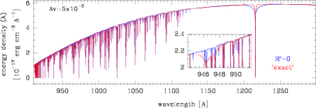
Figure 2: Radiative transfer models for a cloud with a total extinction of A_V=1 and a density of $n_{H}$=10³ cm^-3, illuminated at both sides by the mean ISRF. Part of the resulting FUV spectra ($\sim$912-1300 Å) close to the cloud surface is shown. The blue spectra correspond to a model with R’=0 in Eq. (16) (depth dependence neglected), and the red one corresponds to the new ”exact” computation.

4 Applications: Comparison with previous approaches

In this section we compare the main differences of the new exact computation versus the line–plus–continuum approach ($\mathbf{R}^{\prime}=0$) used by Le Petit et al. (2006) in the Meudon PDR code. Since the previous version of the code used a single–dust albedo and $g$–asymmetry parameter with no wavelength or depth dependence, and the extinction curve was not related to the grain properties used in the model, here we just make the comparison by assuming $\mathbf{R}^{\prime}=0$ in the new computation, and limit ourselves to the uniform dust properties case. In the following examples we explicitely include all the H, H₂ and CO electronic absorption lines arising from rotational levels up to $J$=6 (for H₂) and $J$=1 (for CO). The FGK approximation (Federman et al. (1979)) is applied for the rest of levels. Note that the exact method allows one to take into account the overlaps between H, H₂ and CO lines neglected in more crude approaches.

Apart from having a radiative transfer method to consistently solve for the dust grain varying populations problem (Section 5), the next largest difference between the new computation compared to Le Petit et al. (2006) is the effect of line–wing absorption of back–scattered radiation. At line core wavelengths, photons penetrating into the cloud are purely absorbed by the gas (the effective albedo equals 0). Due to saturation and opacity broadening, many absorption lines become very wide deep inside the cloud. As a consequence, the FUV radiation field is more attenuated than in the (only) dust continuum transfer case. At continuum wavelengths free of lines, a fraction of photons coming from the external illumination sources can be absorbed by the dust (depending on the exact dust albedo value) or be back–scattered (depending on the exact $g$ value) and provide an additional contribution to the radiation field at the cloud surface (about 10% of increase for $g=<\cos\theta>\simeq 0.6$). At line wing wavelengths, where dust and gas opacities are of the same order (and the effective albedo is in between 0 and the grain albedo), some of the back–scattered photons can again reach the surface of the cloud while another fraction will be absorbed in the wings. Therefore, as shown by our calculations, line wings are ”numerically more challenging”. The fraction of absorbed photons in the line wings depends on the wavelength separation to the line core and on the transition upper level life time (because it determines the resulting line profile broadening). To illustrate these differences we consider a cloud with a constant density $n_{H}$=10³ cm^-3 and a total extinction depth of $A_{V}$=1, illuminated at both sides by the mean interstellar radiation field (ISRF, $\chi=1$) as defined by Draine (1978). These physical conditions resemble those of a diffuse cloud such as parts of $\zeta$ Ophiuchi (e.g. Black & Dalgarno (1977)). An uniform grain size distribution similar to that of Mathis et al. (1977) is assumed. Figure 2 shows part of the resulting FUV spectra ($\sim$912-1300 Å) close to the cloud surface. These spectra clearly show that the effect of H₂ line wing absorption of back-scattered photons is larger in the exact computation compared to the $\mathbf{R}^{\prime}=0$ approach (Le Petit et al. (2006)). Note that this is true only for $H_{2}$ lines. Atomic hydrogen lines exhibit the opposite effect, i.e. a decrease of the line wing absorption of back-scattered photons compared to the $\mathbf{R}^{\prime}=0$ approach. Figure 10 shows the impact of the same two, exact and $\mathbf{R}^{\prime}=0$, computations in the resulting cloud structure (left: H/H₂ transition and right: H₂ photodissociation rate). In spite of the different line profiles predicted by each type of model, the final cloud physical conditions remain very similar. Therefore, we conclude that all computations made with the previous version of the Meudon PDR code (Le Petit et al. (2006)), where line transfer was computed (assuming $\mathbf{R}^{\prime}=0$ and uniform dust properties), are consistent with the present exact calculation. The larger effect of the H₂ line–wing absorptions in the exact calculation increases the attenuation of the illuminating radiation field, which results in a H/H₂ transition layer slightly shifted to lower extinction depths. This general result obviously applies to any FUV radiative transfer model including gas line absorption compared to (only dust) continuum models, i.e. the contribution of gas absorption (H₂ lines mostly) decrease the photoionization rate (of neutral carbon particularly) and the photodissociation rate of species with thresholds close to the Lyman cut. An adventage of including gas line absorption is that predicted spectra can be directly compared with spectral observations provided by FUV telescopes.

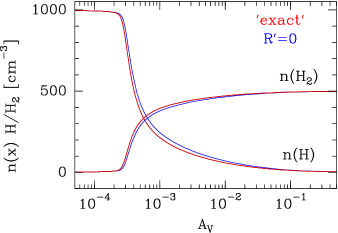
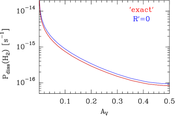
Figure 3: Impact of the new ’exact’ radiative transfer computation compared to an alternative approach that assumes $R^{\prime}$=0 (Le Petit et al. (2006)). Grain properties are uniform in all the cloud (MRN). Left panel: H/H₂ transition. Right panel: H₂ photodissociation rate as a function of cloud depth. A cloud with a density of $n_{H}$=10³ cm^-3, a total extinction depth of A_V=1 and illuminated at both sides by the mean ISRF is considered. These results show that for the case of uniform dust grain properties the error associated with $R^{\prime}$=0 assumption is small.

5 Applications: Grain growth, varying dust populations

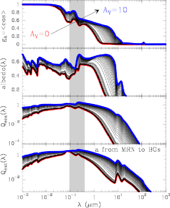
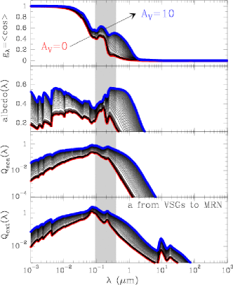
Figure 4: Grains mixture optical parameters as a function of wavelength and cloud depth (the red curve corresponds to the illuminated cloud edge A_V=0 and the blue curve to the center of the cloud at A_V=10) for the ”MRN to BGs” (left) and ”VSGs to MRN” (right) examples respectively. The shaded region shows the spectral region taken into account in the FUV radiative transfer.

With the method presented in Sec. 3, we can now consistently explore the effect of more realistic (non–uniform) dust properties in the FUV penetration into more embedded objects e.g., dense molecular clouds or protoplanetary disks. As a representative example, we present several models for a dense and strongly illuminated cloud (with an ionization parameter of $\chi/n_{H}=1$ cm³) with grain radii varying dust populations. From the chemical point of view we only concentrate here on the effects that the different FUV attenuation depths have on the classical H/H₂ and C⁺/C/CO layered structures predicted by PDR models. In particular, we consider a cloud with a constant density $n_{H}=n(H)+2\,n(H_{2})$=10⁵ cm^-3 and a total extinction of $A_{V}$=20 which is illuminated at both sides by 10⁵ times the ISRF. These physical conditions resemble those of a dense PDR such as the Orion Bar (e.g. Tielens & Hollenbach (1985)) or a photoevaporating disk around a massive star (e.g. Johnstone, Hollenbach, & Bally 1998). At any depth we consider that dust grains follow a size distribution $dn=n_{a}\,da$ given by:

$$n_{a}(\tau)=\sum_{i}n_{a,i}(\tau)=\sum_{i}A_{i}(\tau)\,n_{H}(\tau)\,a^{-\beta_{i}}\,da\hskip 28.45274pta_{i,-}(\tau)<a(\tau)<a_{i,+}(\tau)$$ (50)

where a_± refers to the grain radius distribution lower and upper limits and $i=1,...,n$ refers to each component of the grain mixture. In Eq. (50) we have explicitly particularized for the simple power–law case, although more complicated problems may require other prescriptions of $n_{a}$ (e.g. such as those in Weingartner & Draine (2001)). Grain properties were taken from Laor & Draine (1993) for silicates and graphite. With these tabulations we compute the optical parameters of the grain mixture for each wavelength and cloud depth. In particular, we compute the $Q_{abs}$, $Q_{sca}$ and $Q_{ext}$ efficiencies and the grain albedo $Q_{sca}/Q_{ext}$. We finally use an $g_{\lambda}$–asymmetry factor averaged over the grain distribution as (see e.g., Wolfire & Cassinelli (1986)):

$$g_{\lambda}(\tau)=\frac{\int_{a_{-}(\tau)}^{a_{+}(\tau)}\,\sum_{i}\pi\,a^{2}\,g_{i}(a,\lambda,\tau)\,Q_{sca}(a,\lambda,\tau)\,\,n_{a,i}(\tau)\,da}{\int_{a_{-}(\tau)}^{a_{+}(\tau)}\,\sum_{i}\pi\,a^{2}\,Q_{sca}(a,\lambda,\tau)\,\,n_{a,i}(\tau)\,da}$$ (51)

Afterwards, the extinction curve $A(\lambda,\tau)/A_{V}(\tau$) and the absolute dust extinction coefficient $\alpha^{d}_{\lambda}(\tau)$ are determined at each depth and used to settle the total line–plus–continuum opacity (as defined in Eq. 2) and the effective albedo. The dust extinction coefficient (cm^-1) is given by $\alpha_{d}(\lambda,\tau)=n_{g}\,\pi a^{2}\,Q_{ext}$, where $n_{g}$ is the number of dust grains (per cm³). Thus, we compute:

$$\alpha_{d}(\tau)=\int_{a_{-}(\tau)}^{a_{+}(\tau)}\pi\,a^{2}\left(\sum_{i}Q_{ext}^{i}(a,\tau)A_{i}(\tau)\,n_{H}(\tau)\,a^{\beta}\right)da$$ (52)

The A${}_{i}(\tau)$ grain coefficients are determined at each depth position assuming that the gas–to–dust mass ratio has to be constant ($\sim$100) in the whole cloud (i.e., the number of grains is reduced if grain sizes increase). However, in order to keep the grain mixture homogeneous, the A_Sil/A_Gra ratio is kept fixed. Contribution of discrete absorption lines, i.e. the contribution of $\alpha^{g}_{\lambda}(\tau)$, is included in similar fashion as described in Le Petit et al. (2006; Sec. 4.3). The total opacity at each depth is then given by:

$$d\tau_{\lambda}=\left(1+\frac{\alpha^{g}}{\alpha^{d}}\right)\frac{A(\lambda)}{A_{V}}\,d\tau_{V}=\left(1+\frac{\alpha_{\lambda}^{g}}{\alpha_{\lambda}^{d}}\right)\left(\frac{E_{\lambda-V}}{E_{B-V}}\,\frac{1}{R_{V}}\,+1\right)\,d\tau_{V}$$ (53)

where all the variables are depth dependent and where we have assumed that, in the visible band, the extinction is only produced by dust and therefore we use $d\tau_{\lambda}=\frac{A(\lambda)}{A_{V}}\,d\tau_{V}=\alpha_{\lambda}^{d}\,ds$ to relate the spatial scale with extinction depth. Note that we compute the extinction curve, at each cloud position, directly from the derived grain properties.

For this ”grain growth example” we consider that grain radii increase as a function of the cloud depth according to:

$$a_{i,\pm}(\tau)=a_{i,\pm}(0)+[a_{i,\pm}(\tau_{c})-a_{i,\pm}(0)]\,\left(\frac{\tau}{\tau_{c}}\right)^{\gamma_{\pm}}$$ (54)

where $a_{i,\pm}(0)$ defines the grain radii at the edge of the cloud ($\tau=0$) and $a_{i,\pm}(\tau_{c})$ refers to the grain radii at the center of the cloud. We chose $\gamma_{\pm}$=2/3. Obviously, this is just an illustrative example since we do not explicitly solve for the grain nucleation/growth (e.g. Salpeter (1974)) nor the erosion/sputtering problem (e.g. Barlow (1978)), which depends on the particular type of source. The crucial point here is to provide a method to consistently solve for the FUV radiative equation if, as suggested by observations, the grains size distribution changes toward embedded objects (Moore et al. (2005)) and/or if spatial fluctuations of the gas to dust ratio do exist along the line of sight (Padoan et al. (2006)).

In the following, grains follow a power–law distribution of sizes given by Eq. (50) with $\beta_{i}$=3.5 at each cloud position. A mixture of silicates and graphite grains defined by $A_{Sil}/A_{Gra}=1.1$ and with $a_{-}(A_{V}=0)$=5 nm, $a_{+}(A_{V}=0)$=250 nm and $a_{-}(A_{V}=10)$=50 nm, $a_{+}(A_{V}=10)$=2500 nm was selected. Therefore, the grain mixture at A_V=0 corresponds to the size distribution proposed by Mathis, Rumpl & Nordsieck (1977; this size distribution is called MRN hereafter) to fit the mean galactic extinction curve (see also Fitzpatrick & Massa (1990)). At A_V=10 grains have grown by a factor 10 and we call them Big Grains (BGs). In the second example we only change the size distribution to $a_{-}(A_{V}=0)$=1 nm, $a_{+}(A_{V}=0)$=50 nm and $a_{-}(A_{V}=10)$=5 nm, $a_{+}(A_{V}=10)$=250 nm. Thus, the grain mixture at A_V=0 corresponds to very small grains (VSGs). At A_V=10 grains have grown by a factor of 5 and follow a MRN distribution again. The third final example considers a uniform grain size distribution (MRN) in the whole cloud. The resulting optical properties, extinction curves, dust opacities, A_i coefficients and radii distributions for these examples are shown in Figs. 4, 5, 6 and 7 (left panel), respectively.

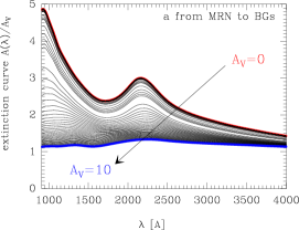
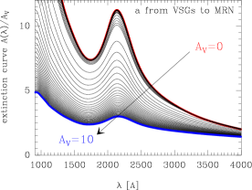
Figure 5: Resulting extinction curves as a function of wavelength (only the FUV range is shown) and cloud depth (the red curve corresponds to the cloud edge A_V=0 and the blue curve to A_V=10) for the ”MRN to BGs” (left) and ”VSGs to MRN” (right) examples respectively.

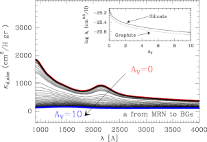
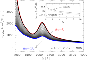
Figure 6: Dust mass absorption coefficients (per gas gr) as a function of wavelength and cloud depth (the red curve corresponds to the cloud edge A_V=0 and the blue curve to A_V=10) for the ”MRN to BGs” (left) and ”VSGs to MRN” (right) examples respectively. The different grain material A_i coefficients required to keep a constant gas–to–dust mass ratio are also shown as a function of $A_{V}$ in the small insets.

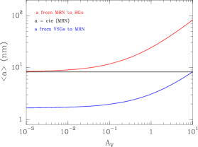
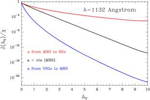
Figure 7: Left: Adopted grain averaged radii distribution for the ”MRN to BGs” (left) and ”VSGs to MRN” (right) examples respectively. Right: Resulting mean intensity of the FUV continuum (at $\sim$1132 Å) as a function of the cloud depth for the three different varying grain populations discussed in the text. The ordinate shows the mean intensity normalized by the illuminating radiation field ($\chi$=10⁵ in Draine’s units).

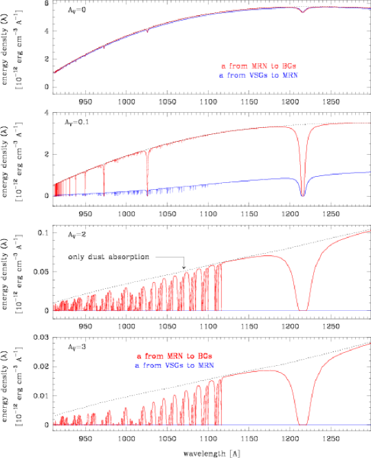
Figure 8: Radiative transfer models for a cloud with a total extinction of A_V=20 and a density of $n_{H}$=10⁵ cm^-3, illuminated at both sides by 10⁵ times the mean ISRF. Part of the resulting FUV spectra ($\sim$912-1300 Å) at different extinction depths: A_V=0 (cloud surface), A_V=0.1, A_V=2 and A_V=3 are shown in each box. In each panel, the red (blue) curve corresponds to the ”MRN to BGs” (”VSGs to MRN”) example.

Some time ago, Sandell & Mattila (1975) emphasized that the albedo and anisotropy of dust grain scattering have important effects on photodissociation rates for ISM molecules.The present computation of the FUV radiation field (continuum+lines) at each cloud position (see Fig. 8 for the resulting FUV spectra at different A_V) allows an explicit integration of consistent C photoionization rates together with H₂ and CO photodissociation rates. Once the FUV radiation field has been determined and the photo rates calculated, steady-state chemical abundances are computed for a given network of chemical reactions. Finally, we compute the thermal structure of the cloud by solving the balance between the most important gas heating and cooling processes (Le Bourlot et al. (1993); Le Petit et al. (2006) and references therein).

Depending on the grain properties these examples show FUV radiation fields that change by orders of magnitude at large A_V (Fig. 7 right panel). Note that the mean radiation intensity at the cloud surface $J(0)$ cannot be larger than the illuminating radiation field itself, i.e., $J(0)/\chi<1$. The exact ratio depends on the particular dust scattering properties ($\sim$0.53-0.54 for these models of optically thick clouds). The influence of the different grain distributions in the attenuation of FUV radiation is obvious, the FUV penetration depth is larger when dust scattering is more efficient, i.e., when grain albedo and scattering anisotropy increase (as dust grains grow toward bigger grains). Note that the only difference between models is the change of grain size distributions across the cloud. Therefore, the assumption of uniform dust properties and averaged extinction curves can be one of the crudest approximations made to determine the resulting cloud physical and chemical state. Figure 9 shows the impact of the different grain growth curves on the resulting cloud structure: kinetic temperature, H₂ photodissociation rate, C photoionization rate and CO photodissociation rates (left column), H/H₂ transition, and C⁺/C/CO abundances (right column). The different intensities of the FUV radiation field for each dust population result in very different photoionization and photodissociation rates which ultimately determine the prevailing chemistry. This conclusion qualitatively agrees with earlier calculations for ISM diffuse clouds (Roberge, Dalgarno & Flannery (1981)) and should be extended to more embedded objects where there are observational evidences (e.g. Moore et al. (2005)) of flatter extinction curves (consistent with grain growth). The H/H₂ and C⁺/C layered structures in our models are different even in similar sources (same density and illumination) if grain properties significantly disagree, or if dust grains vary along the observed region. Different ionization fractions, molecular ions enhancements, and C⁺/C/CO abundances should thus be observed. In particular, photochemistry can still be important at large A_V if anisotropic scattering of the illuminating radiation is efficient (e.g., ”MRN to BGs” model). In this case, CO photodissociation and carbon ionization still dominate the CO destruction and C⁺ formation respectively deeper inside the cloud. As a result, the predicted abundance of neutral and ionized carbon at A_V=10 is enhanced compared to standard MRN dust models (see Fig. 9).

Secondly, the intensity of the FUV radiation field also determines much of the thermal structure of the cloud through the efficiency of the grain photoelectric effect, the dominant heating mechanism (e.g. Draine 1978). Since FUV radiation penetrates deepest when dust grains are bigger, the photoelectric heating rate is kept high deeper inside the cloud. Thus, a larger fraction of the gas is maintained warm at large extinction depths. Warmer temperatures also affect the rates of chemical reactions with activation energy barriers. For the smallest dust grains, FUV attenuation is so high that photoelectric heating soon becomes inefficient and the gas is colder at large extinctions depths. Note that since grain ionization is very large in the surface of the cloud (due to the high illumination in the selected example), the maximum efficiency of the photoelectric effect, i.e. the maximum temperature, is reached deeper inside the cloud where the grain ionization has decreased. The general effects described here must play a significant role in illuminated sources where grain growth takes place, specially in protoplanetary disks, circumstellar envelopes around evolved stars and dense molecular clouds near H ii regions. In these cases, the FUV penetration depth is increased if dust grains evolve toward bigger grains, leading to larger photochemically active regions.

Conversely, molecular species such as CO will be more abundant in irradiated regions where the smallest grains dominate the extinction efficiency. Figure 10 shows the effects of grain growth in a diffuse cloud (A_V=1), with a density of $n_{H}$=10³ cm^-3, and illuminated by the mean ISRF. Although the resulting variations are not so large compared to optically thick clouds, the different photoionization and photodissociation rates also translate into different atomic and molecular abundances.

In particular, the C⁺/C and C⁺/CO abundance ratios change up to a factor $\sim$10 depending on the assumed grain properties. Note that for optically thin clouds, the mean intensity at one surface can have a significant contribution from the other side illumination (that increases with the scattering efficiency). As an example, the mean intensity at A_V=0 in the ”MRN to BGs” grain model ($J(0)/\chi$$\simeq$0.63; red curves in Fig. 10) is a factor $\sim$$20\%$ larger than in the ”VSGs to MRN” model (blue curves). This effect slightly modifies the dissociation and ionization rates at the cloud surface.

In summary, as gas photodissociation and heating determine much of the chemistry in FUV irradiated gas, the resulting source structure is severely altered by the assumed (or observed) grain properties. Therefore, understanding dust properties and grain variations in individual sources is a crucial step to determine the source physical and chemical state.

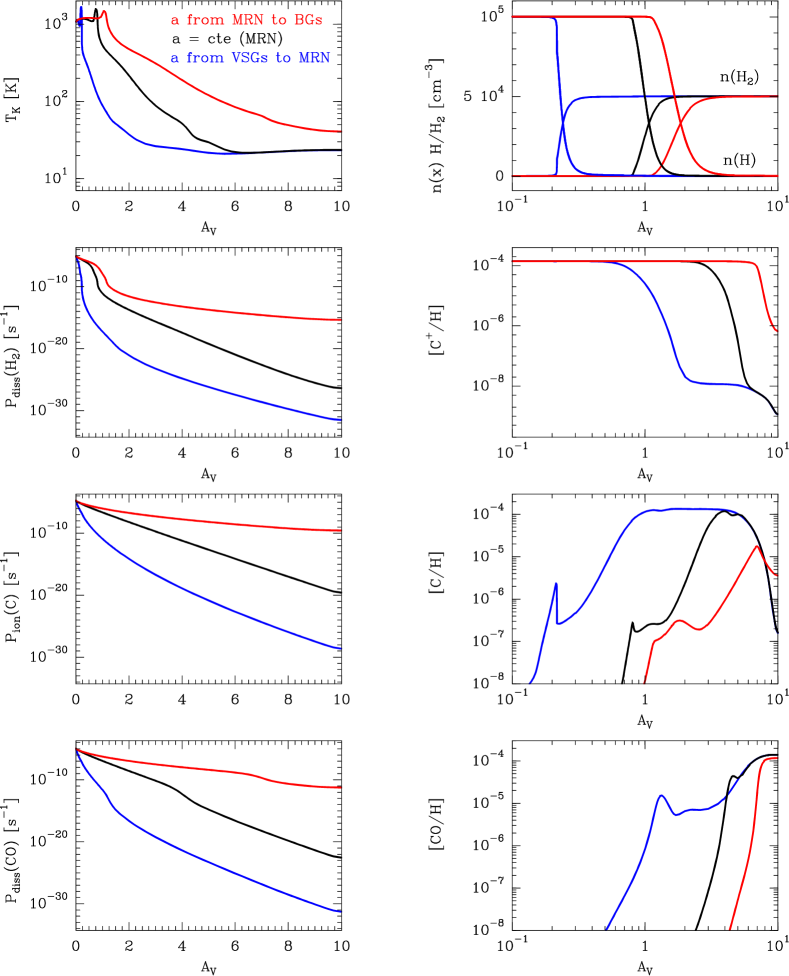
Figure 9: Impact of the different FUV radiative transfer models on the kinetic temperature, H₂ photodissociation rate, C photoionization rate and CO photodissociation rate (left column), H/H₂ transition and C⁺/C/CO column densities (right column). A cloud with a density of $n_{H}$=10⁵ cm^-3, a total extinction depth of A_V=20 and illuminated at both sides by 10⁵ times the mean ISRF is considered. Although not clearly seen in these boxes, all physical parameters show an horizontal tangent at Av = 10, consistent with their null variation with respect to the depth position at half cloud (as expected for a symmetrically illuminated cloud).

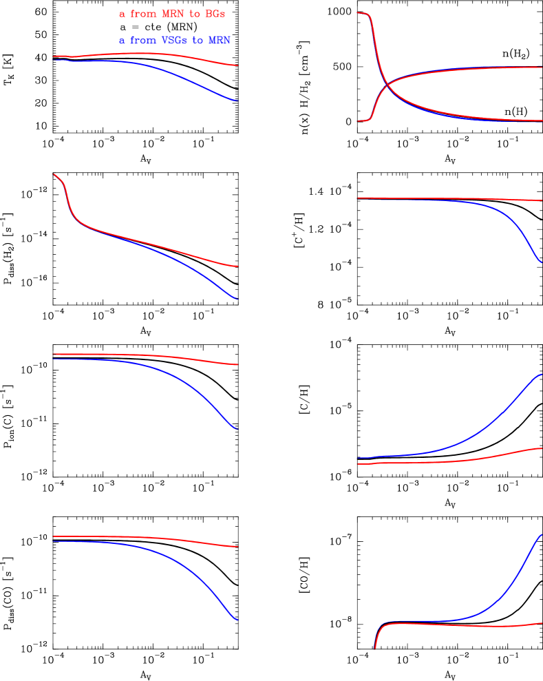
Figure 10: Same as Figure 9 for a cloud with $n_{H}$=10³ cm^-3, a total extinction depth of A_V=1 and illuminated at both sides by the the mean ISRF. Dust grains grow according to Eq. (54) with A${}_{V}^{c}$=1.086 $\tau_{V}^{c}$=0.5.

6 Summary and conclusions

1. An extension of the spherical harmonics method to solve for the radiative transfer equation with depth dependent coefficients in plane–parallel geometry has been presented. The method can be used to solve for the FUV radiation field in externally or internally illuminated clouds, taking into account gas absorption and coherent, nonconservative and anisotropic scattering by dust grains. Our extended formulation thus allows to consistently include $(i)$ gas lines and $(ii)$ varying dust populations.

2. We have shown that the penetration of FUV radiation is heavily influenced by dust properties. According to the dust ISM and CSM life–cycle, such properties likely change from source to source but also they change within the same object. The FUV penetration depth rises for increasing dust albedo and anisotropy of the scattered radiation when grains grow at large A_V (as suggested observationally). Therefore, the modeled physical and chemical state of illuminated molecular clouds, protoplanetary disks or entire galaxies can be altered by large factors if a more realistic treatment of the interaction between radiation and matter is considered.

3. The new formulation has been implemented in the Meudon PDR code and thus it will be publicly available. Particular examples where only the dust populations are changed show intensities of the FUV radiation field that differ by orders of magnitude at large A_V. Therefore, the resulting photochemical and thermal structures of molecular clouds can be very different depending on the assumed grain properties and growth.

Appendix A Inclusion of embedded sources of emission ($S^{*}\neq 0$)

In this appendix we give the recipe to include the true emission by ”embedded sources of photons” in the method described in section 3. In this case the source function includes the scattering of photons by dust grains plus a non null $S^{*}_{\lambda}=\frac{j_{\lambda}}{\alpha_{\lambda}+\sigma_{\lambda}}$ term (see Eq. 3 and Fig. 1), where $j_{\lambda}(s)$ is the emission coefficient (line or continuum) of any source of internal radiation.

Firstly, the angular dependence of $S^{*}(\tau,\mu)$ has to be also expanded in a truncated series of Legendre polynomials $P_{l}(\mu)$ as:

$$S^{*}(\tau,\mu)=\sum_{l=0}^{L}(2l+1)\,s_{l}(\tau)\,P_{l}(\mu)$$ (55)

where the dependence with $\lambda$ is omitted. The inclusion of Eqs. (55) into the transfer equation (3) leads to an additional term in the set of coupled, linear, first order differential equations in the unknown $f_{l}(\tau)$ coefficients:

$$lf^{\prime}_{l-1}(\tau)+(l+1)f^{\prime}_{l+1}(\tau)=(2l+1)\,[1-\omega(\tau)\sigma_{l}(\tau)]\,f_{l}(\tau)-(2l+1)\,s_{l}(\tau)$$ (56)

Therefore, the system of equations (56) is now non-homogeneous and can be written as:

$$\mathbf{f^{\prime}}(\tau)=\mathbf{A^{-1}\mathnormal{(\tau)\,}f}(\tau)+\mathbf{A^{-1}\mathnormal{(\tau)\,}g}(\tau)$$ (57)

where $g_{l}(\tau)=-s_{l}(\tau)/(1-\omega(\tau)\,\sigma_{l}(\tau))$. Although the method can be easily used for anisotropic source functions, in most practical applications, the embedded sources of photons emit isotropically and therefore the terms in the expansion of $S^{*}(\tau)$ in Eq. (55) reduce to $s_{l}(\tau)=S^{*}(\tau)\,\delta_{l0}$, and thus, $g_{l}(\tau)$ reduces to $g_{0}(\tau)=-S^{*}(\tau)/(1-\omega(\tau))$ with $g_{l}(\tau)=0$ if $l\neq 0$. Using the same set of auxiliary variables $\mathbf{y}(\tau)=\mathbf{R^{-1}}(\tau)\,\mathbf{f}(\tau)$, Eq. (16) is now written as:

$$\mathbf{y^{\prime}}=\mathbf{K}\,\mathbf{y}-\mathbf{R}^{-1}\,\mathbf{R}^{\prime}\,\mathbf{y}+\mathbf{K}\,\mathbf{R}^{-1}\,\mathbf{g}$$ (58)

Note that by inserting $\mathbf{R}\mathbf{R}^{-1}$ between $\mathbf{A}^{-1}$ and $\mathbf{g}$, we have simplified $\mathbf{R}^{-1}\,\mathbf{A}^{-1}\,\mathbf{g}$ as $\mathbf{K}\,\mathbf{R}^{-1}\,\mathbf{g}$. This result is particularly useful, since it avoids computing $\mathbf{A}^{-1}$ completely. Hence, the last matrix product, $\,\widetilde{\mathbf{Q}}=\mathbf{K}\,\mathbf{R}^{-1}\,\mathbf{g}$, makes the system non–homogeneous:

$$y^{\prime}_{m}=k_{m}(\tau)\,y_{m}+[\mathbf{L\,y}]_{m}(\tau)+\widetilde{q}_{m}(\tau)$$ (59)

Eq. (59) can also be solved with the iterative scheme described in section 3 by including the additional $\widetilde{q}_{m}$ term, i.e.,

$$y_{m}^{(n+1)}(\tau)=e^{\int_{\tau_{m}}^{\tau}\,k_{m}(t)\,dt}\left[C_{m}^{(n+1)}+\int_{\tau_{m}}^{\tau}\,e^{-\int_{\tau_{m}}^{t}\,k_{m}(t^{\prime})\,dt^{\prime}}\,\left([\mathbf{L\,y}^{(n)}]_{m}(t)+\widetilde{q}_{m}(t)\right)dt\right]$$ (60)

It is straightforward to show that the $f_{l}(\tau)$ terms in the Legendre expansion of the radiation field $I(\tau,\mu)$ are still given by Eq. (29). The only change compared to the $S^{*}$=0 case is that the $q_{m}(\tau)$ variables in the $D_{m}^{-}(\tau)$ and $D_{m}^{+}(\tau)$ integrals (Eqs. 25 and 26) have to be substituted by $q_{m}(\tau)-\widetilde{q}_{m}(\tau)$, that is:

$$D_{m}^{-}(\tau)=\int_{0}^{\tau}\frac{E_{m}^{-}(\tau)}{E_{m}^{-}(t)}\,\left(q_{m}(t)-\widetilde{q}_{m}(t)\right)\,dt\qquad(m<0)$$ (61)

$$D_{m}^{+}(\tau)=\int_{\tau}^{\tau_{max}}\frac{E_{m}^{+}(\tau)}{E_{m}^{+}(t)}\,\left(q_{m}(t)-\widetilde{q}_{m}(t)\right)\,dt\qquad(m>0)$$ (62)

The iterative procedure can now be initiated taking into account that at large optical depths the intensity of the radiation field is isotropic and tends to the ratio of the true emission to the true absorption:

$$I(\tau\rightarrow\infty)\simeq\frac{S^{*}(\tau)}{1-\omega(\tau)}\delta_{l0}$$ (63)

In practice, the assumption $\tau\rightarrow\infty$ may be too crude. We have computed that by adding the effect of the external radiation that penetrates deepest into the cloud, the iterative scheme is more robust. Therefore, the first set of $y_{m}(\tau)$ variables in the iterative procedure, $y_{m}^{0}(\tau)$, are computed from the linear system:

$$\sum_{m=-M}^{+M}R_{lm}(\tau)\,y_{m}^{0}(\tau)=f_{l}^{approx}(\tau)=\frac{s_{0}(\tau)}{1-\omega(\tau)}+\frac{1}{2}I(0,-1)\,\exp[-k_{1}(\tau)\,\tau]+\frac{1}{2}I(\tau_{max},1)\,\exp[k_{-1}(\tau)(\tau_{max}-\tau)]$$ (64)

where only the $l=0$ terms are considered.

We have successfully applied the above method by associating $S^{*}$ to thermal emission of dust. These kind of computations are useful if the radiative transfer calculation is extended to the IR domain ($\lambda>1\leavevmode\nobreak\ \mu$m), where scattering of IR photons by dust grains is still significative. In the FUV domain, $S^{*}$ can represent any source of internal illumination. In a future paper we plan to include ”secondary” line photons in the embedded source function. This line FUV radiation field arises from the H₂ radiative de-excitations that follow the H₂ excitation by collisions with electrons and cosmic rays (Prasad & Tarafdar (1983)) and is generally poorly treated. However, it constributes to molecular photodissociation deep inside molecular clouds where the continuum FUV radiation field has been attenuated.

Appendix B Numerical solution and error limits

In Sec. 3.2.1 we turn the system of differential equations (17) into and integral problem (Eqs. 18) that we solve numerically through an iterative scheme (Eqs. 20). In this appendix we provide a bound on the error associated with this procedure and we verify that the derived solution satisfies the original system of equations (10).

Given a numerical approximation $y_{m}^{(n)}$ to the true solution $y_{m}$, we investigate if our iterative proccess converges for all $\lambda$ and $A_{V}$ of the wavelength and cloud depth grids. Thus, we compute:

$$y_{m}^{(n+1)}(\tau)=e^{a_{m}(\tau)}\left[C_{m}^{(n+1)}+\int_{\tau_{m}}^{\tau}\,e^{-a_{m}(t)}\,[\mathbf{L\,y}^{(n)}]_{m}(t)\,dt\right]\hskip 22.76228pt$with$\hskip 22.76228pt\left[\mathbf{Ly}^{(n)}\right]_{m}(t)=\sum_{i=-M}^{+M}L_{mi}(t)\,y_{i}^{(n)}(t)$$ (65)

and write the error in step $n+1$ as $\Delta_{m}^{(n+1)}=y_{m}-y_{m}^{(n+1)}$ where $m=\pm 1,...,\pm M$. Note that this is the difference between the true $y_{m}$ (unknown) and our numerical approximation at step $n+1$. Since the above equations are linear, $\Delta_{m}^{(n+1)}$ reduces to:

$$\Delta_{m}^{(n+1)}(\tau)\simeq e^{a_{m}(\tau)}\,\sum_{i=-M}^{+M}\,\left(\int_{\tau_{m}}^{\tau}e^{-a_{m}(t)}\,L_{mi}(t)\,\Delta_{i}^{(n)}(t)\,dt\right)$$ (66)

because the boundary conditions term ($C_{m}-C_{m}^{(n+1)}$) is small and damped almost everywhere by the exponential term (as shown numerically). If we now define $\Delta_{i}^{(n),MAX}=\max_{t}|\Delta_{i}^{(n)}(t)|$, the maximum error at iteration step $n$ in the Legendre expansion of order $i$ ($i=0,1,...,L$) at any depth position, then:

$$\Delta_{m}^{(n+1),MAX}<\sum_{i=-M}^{+M}\,\Delta_{i}^{(n),MAX}\,\left(\int_{\tau_{m}}^{\tau}e^{\left[a_{m}(\tau)-a_{m}(t)\right]}\,L_{mi}(t)\,dt\right)$$ (67)

By taking the maximum error at iteration step $n$ at any depth position and at any Legendre order, $\Delta^{(n),MAX}=\max_{m}\Delta_{m}^{(n),MAX}$, we arrive to a severe upper limit to the error between the true solution and the numerical approximation at step $n+1$:

$$\Delta^{(n+1),MAX}<\Delta^{(n),MAX}\,\sum_{i=-M}^{+M}\,\left(\int_{\tau_{m}}^{\tau}e^{\left[a_{m}(\tau)-a_{m}(t)\right]}\,L_{mi}(t)\,dt\right)=\Delta^{(n),MAX}\,\cdot\,\mathcal{A}$$ (68)

Therefore, convergence is guaranteed if $\mathcal{A}<1$ as $\Delta^{(n+1),MAX}<\Delta^{(1),MAX}\,\mathcal{A}^{n}$. Obviously convergence occurs also for less restrictive conditions but this is harder to constrain. In our computations we find $\mathcal{A}<1$ for almost all wavelengths and depth positions. Only at some specific locations in the ($A_{V}^{\lambda}$) grid (those associated with some line wings), $\mathcal{A}$ can take values $<10$. However, a close look at successive variations of $\Delta_{m}^{(n+1)}-\Delta_{m}^{(n)}$ at those locations shows that $\Delta_{m}^{(n+1)}-\Delta_{m}^{(n)}$ is effectively null after a few iterations.

A final test to validate our numerical solution is to compute the numerical derivative of our solution and compare $\mathbf{f}$ with $\mathbf{A}\,\mathbf{f^{\prime}}$ (see Eq. (10)). Although grain properties are kept uniform, inclusion of gas absorption makes $\mathbf{R}^{\prime}(\tau)\neq 0$ and thus $\mathbf{L}^{\prime}(\tau)\neq 0$ in Eq. (17). Figure 11 shows a typical example for a test cloud with $A_{V}=1$ and $n_{H}=300\,{\rm cm}^{-3}$, illuminated by the standard radiation field on both sides. In particular, we compare the $f_{l}$ ($l$=0) component of $\mathbf{f}$ with $\mathbf{A}\,\mathbf{f}^{\prime}$ at $\lambda=914.26\,\textrm{\AA}$, a ${\rm H}_{2}$ line wing with a total optical depth of 80. Hence, variations of physical conditions along the cloud are large. It can be seen that the agreement is excellent. In a continuum ”free of lines” wavelength range, agreement is perfect, and there is nothing to show. Hence, the derived numerical solution is a very good approximated solution to the radiative transfer problem.

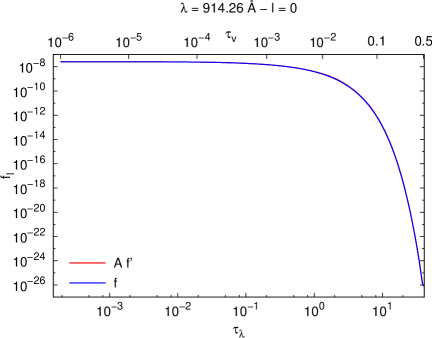
Figure 11: Comparison of $\mathbf{f}$ and $\mathbf{A}\,\mathbf{f^{\prime}}$ for $l$=0 and $\lambda=914.26\,\textrm{\AA}$. The abscissa corresponds to $\tau_{v}$ for the upper scale and to $\tau_{line}$ for the lower scale.

Appendix C Eigenvalues and eigenvectors of $\mathbf{A^{-1}}(\tau)$

We describe here our method to compute the eigenvalues and eigenvectors of the $\mathbf{A^{-1}}(\tau)$ matrix (see Eq.(13)). Note that $\mathbf{A}(\tau)$ and $\mathbf{A}^{-1}(\tau)$ have the same eigenvectors, but $k_{m}^{-1}(\tau)$ and $k_{m}(\tau)$ eigenvalues respectively.

A first trick is to turn this diagonalization problem to a symmetric problem. Let us call $\mathbf{R}_{m}(\tau)$ an eigenvector of $\mathbf{A}(\tau)$ with $R_{lm}(\tau)$ components and $k_{m}^{-1}(\tau)$ eigenvalues. Thus, $\mathbf{R}(\tau)$ is the matrix formed by the $\mathbf{R}_{m}(\tau)$ eigenvectors and we can write:

$$\left(\begin{array}[]{cccccc}0&h_{0}^{-1}&.&.&.&.\\ h_{1}^{-1}&0&2h_{1}^{-1}&.&.&.\\ .&2h_{2}^{-1}&0&\ddots&.&.\\ .&.&3h_{3}^{-1}&\ddots&(L-1)h_{L-2}^{-1}&.\\ .&.&.&\ddots&0&Lh_{L-1}^{-1}\\ .&.&.&.&Lh_{L}^{-1}&0\end{array}\right).\left(\begin{array}[]{c}R_{0m}\\ R_{1m}\\ R_{2m}\\ \vdots\\ R_{L-1,m}\\ R_{Lm}\end{array}\right)=k_{m}^{-1}(\tau)\,\left(\begin{array}[]{c}R_{0m}\\ R_{1m}\\ R_{2m}\\ \vdots\\ R_{L-1,m}\\ R_{Lm}\end{array}\right)$$

with $h_{l}(\tau)=(2l+1)\,(1-\omega(\tau)\sigma_{l}(\tau))$. If we now define $\mathbf{G}(\tau)$ as diagonal matrix with $g_{ll}(\tau)=h_{l}^{1/2}(\tau)$, left-multiplication of the previous equation by $\mathbf{G}(\tau)$ and insertion of the identity matrix ${\rm I}=\mathbf{G}^{-1}(\tau)\,\mathbf{G}(\tau)$ between $\mathbf{A}(\tau)$ and $\mathbf{R}(\tau)$ gives:

$$\left(\begin{array}[]{cccccc}0&\frac{1}{\sqrt{h_{0}h_{1}}}&.&.&.&.\\ \frac{1}{\sqrt{h_{0}h_{1}}}&0&\frac{2}{\sqrt{h_{1}h_{2}}}&.&.&.\\ .&\frac{2}{\sqrt{h_{1}h_{2}}}&0&\ddots&.&.\\ .&.&\frac{3}{\sqrt{h_{2}h_{3}}}&\ddots&\frac{L-1}{\sqrt{h_{L-2}h_{L-1}}}&.\\ .&.&.&\ddots&0&\frac{L}{\sqrt{h_{L-1}h_{L}}}\\ .&.&.&.&\frac{L}{\sqrt{h_{L-1}h_{L}}}&0\end{array}\right).\left(\begin{array}[]{c}h_{0}^{1/2}R_{0m}\\ h_{1}^{1/2}R_{1m}\\ h_{2}^{1/2}R_{2m}\\ \vdots\\ h_{L-1}^{1/2}R_{L-1,m}\\ h_{L}^{1/2}R_{Lm}\end{array}\right)=k_{m}^{-1}(\tau)\,\left(\begin{array}[]{c}h_{0}^{1/2}R_{0m}\\ h_{1}^{1/2}R_{1m}\\ h_{2}^{1/2}R_{2m}\\ \vdots\\ h_{L-1}^{1/2}R_{L-1,m}\\ h_{L}^{1/2}R_{Lm}\end{array}\right)$$ (69)

This new symmetric matrix is called $\mathbf{\tilde{A}}(\tau)$, and $\mathbf{\tilde{R}}(\tau)$ is the matrix of its eigenvectors. The $\mathbf{\tilde{A}}(\tau)$ matrix has the same eigenvalues $k_{m}^{-1}(\tau)$ as $\mathbf{A}(\tau)$, although the eigenvectors $\mathbf{R}(\tau)$ and $\mathbf{\tilde{R}}(\tau)$ are different but related by $\mathbf{\tilde{R}}(\tau)=\mathbf{G}(\tau)\,\mathbf{R}(\tau)$. These symmetric matrixes are easier to diagonalize numerically. Eigenvectors are computed by the recurrence relation:

$$R_{0m}(\tau)=1$$

$$R_{1m}(\tau)=(1-\omega(\tau))/k_{m}(\tau)$$

$$R_{lm}(\tau)=\frac{1}{lk_{m}(\tau)}\,\left[h_{l-1}(\tau)\,R_{l-1,m}(\tau)-(l-1)\,k_{m}(\tau)\,R_{l-2,m}(\tau)\right]$$ (70)

where, compared to Roberge (1983), $\omega(\tau)$ is a $\tau$–dependent effective albedo including line absorption.

Appendix D Inverse and derivative of $\mathbf{R}(\tau)$

Here we show how $\mathbf{R}^{-1}(\tau)$ is computed. Unfortunately, $\mathbf{A}(\tau)$ is not a symmetric matrix, so that $\mathbf{R}^{-1}(\tau)\neq\mathbf{R}^{T}(\tau)$. However, we can apply the same method as above to turn $\mathbf{R}^{-1}(\tau)$ into $\mathbf{\tilde{R}}^{T}(\tau)$. Since $\mathbf{\tilde{A}}(\tau)$ is symmetric, the matrix formed with its eigenvectors is orthogonal. Thus, using the same notations, we have:

$$\mathbf{\tilde{R}}^{T}(\tau)\,\mathbf{\tilde{R}}(\tau)=\mathbf{J}(\tau)=(\mathbf{G}(\tau)\,\mathbf{R}(\tau))^{T}\,\mathbf{G}(\tau)\,\mathbf{R}(\tau)$$ (71)

where $\mathbf{J}(\tau)$ is a diagonal matrix with $J_{ll}(\tau)=\left\|\mathbf{\tilde{R}}_{l}(\tau)\right\|^{2}$ elements. Hence:

$$\mathbf{R}^{-1}(\tau)=\mathbf{J}^{-1}(\tau)\,\mathbf{R}^{T}(\tau)\,\mathbf{G}^{2}(\tau)$$ (72)

The inclusion of the depth dependence in the spherical harmonics method unfortunately forces to calculate the $\mathbf{R}(\tau)$ derivative respect to $\tau$. Ideally, we could start to derivate the $R_{lm}(\tau)$ recurrence relations shown in Eq (70) to get:

$$R^{\prime}_{0m}=0$$

$$R^{\prime}_{1m}=-\frac{\omega^{\prime}k_{m}+(1-\omega)k^{\prime}_{m}}{k_{m}^{2}}$$

$$R^{\prime}_{lm}=-\frac{k^{\prime}_{m}}{lk_{m}^{2}}\,\left[h_{l-1}R_{l-1,m}-(l-1)k_{m}R_{l-2,m}\right]+\frac{1}{lk_{m}}\,\left[h^{\prime}_{l-1}R_{l-1,m}+h_{l-1}R^{\prime}_{l-1,m}-(l-1)\left(k^{\prime}_{m}R_{l-2,m}+k_{m}R^{\prime}_{l-2,m}\right)\right]$$ (73)

with

$$h^{\prime}_{l}(\tau)=-(2l+1)\,[\omega^{\prime}(\tau)\sigma_{l}(\tau)\,+\omega(\tau)\sigma_{l}^{\prime}(\tau)]$$ (74)

Unfortunately, $\omega^{\prime}$, $\sigma_{l}^{\prime}$ and $k^{\prime}_{m}$ have to be computed also numerically, which is quite unstable in the most external cloud positions due to the large variations of $\tau_{\lambda}$ at line wing wavelengths (where the line opacity becomes comparable to the dust opacity) compared to deeper inside the cloud where $\tau_{\lambda}$ at the same wavelength becomes saturated (the dust opacity becomes insignificant respect to the line opacity). Besides, a symmetric difference scheme does not provide satisfactory results because $\frac{\omega_{n+1}-\omega_{n-1}}{\tau_{n+1}-\tau_{n-1}}$ only gives an approximation to $\omega^{\prime}$ at $\tau=\frac{\tau_{n-1}+\tau_{n+1}}{2}$ which, in general, is not $\tau_{n}$. We solved this problem by derivating directly the computed values of $R(\tau)$. To avoid irregular steps in $\tau$, a second order polynomial was fit to $R_{lm}(\tau_{i-2})$, $R_{lm}(\tau_{i})$ and $R_{lm}(\tau_{i+2})$, and the value of its analytical derivative was then used. The resulting derivative $\mathbf{R}^{\prime}(\tau)$ is smooth enough to be applied in the numerical computation.

Appendix E Mean radiation field intensity

In section 3.4 we deduced the simple form that the mean intensity takes in the spherical harmonics method, i.e. $J(\tau)=f_{0}(\tau)$. However, in some cases of astrophysical interest (e.g. a two sides asymmetrically illuminated cloud) one needs to distinguish the fraction of radiation field coming from each side of the cloud. In this case, two half sums have to be computed. Here we give the analytical expressions that we use to compute $J^{\pm}(\tau)$. For radiation coming from the $\tau=0$ side we have:

$$J^{-}(\tau)=\frac{1}{2}\int_{-1}^{0}I(\tau,\mu)\,d\mu=\frac{1}{2}\,\sum_{l}(2l+1)\,f_{l}(\tau)\,\int_{-1}^{0}P_{l}(\mu)\,d\mu$$ (75)

And for radiation coming from the $\tau=\tau_{max}$ side we have:

$$J^{+}(\tau)=\frac{1}{2}\int_{0}^{+1}I(\tau,\mu)\,d\mu=\frac{1}{2}\,\sum_{l}(2l+1)\,f_{l}(\tau)\,\int_{0}^{+1}P_{l}(\mu)\,d\mu$$ (76)

If we define $\mathcal{Q}_{l}=\int_{0}^{+1}P_{l}(\mu)\,d\mu$, with:

$$\mathcal{Q}_{l}=\left\{\begin{array}[]{lc}1&l=0\\ 0&l\,\,\textrm{even and }>0\\ \frac{P_{l-1}(0)}{l+1}&l\,\,\textrm{odd}\end{array}\right.$$ (77)

parity gives $\int_{-1}^{0}P_{l}(\mu)\,d\mu=(-1)^{l}\,\mathcal{Q}_{l}=-\mathcal{Q}_{l}$ (using $\mathcal{Q}_{l}=0$ for $l$ even). Inserting Eq. (29) in Eqs (75) and (76) we get:

$$J^{-}(\tau)=\frac{1}{2}\sum_{m=-M}^{-1}\left(C_{m}\,E_{m}^{-}(\tau)-D_{m}^{-}(\tau)\right)\,\left(1-\sum_{l=1}^{L}(2l+1)\,\mathcal{Q}_{l}\,R_{lm}(\tau)\right)+\frac{1}{2}\sum_{m=1}^{M}\left(C_{m}\,E_{m}^{+}(\tau)+D_{m}^{+}(\tau)\right)\,\left(1-\sum_{l=1}^{L}(2l+1)\,\mathcal{Q}_{l}\,R_{lm}(\tau)\right)$$ (78)

$$J^{+}(\tau)=\frac{1}{2}\sum_{m=-M}^{-1}\left(C_{m}\,E_{m}^{-}(\tau)-D_{m}^{-}(\tau)\right)\,\left(1+\sum_{l=1}^{L}(2l+1)\,\mathcal{Q}_{l}\,R_{l,m}(\tau)\right)+\frac{1}{2}\sum_{m=1}^{M}\left(C_{m}\,E_{m}^{+}(\tau)+D_{m}^{+}(\tau)\right)\,\left(1+\sum_{l=1}^{L}(2l+1)\,\mathcal{Q}_{l}\,R_{lm}(\tau)\right)$$ (79)

Taking into account the fact that $\mathcal{Q}_{l}=0$ if $l$ is even, and $R_{l,-m}=-R_{lm}$ if $l$ is odd, we now define (for $m>0$)

$$\mathcal{S}_{m}(\tau)=\sum_{l\,odd}(2l+1)\,\mathcal{Q}_{l}\,R_{l,m}(\tau)$$ (80)

to write:

$$J^{-}(\tau)=\frac{1}{2}\sum_{m=-M}^{-1}\left(C_{m}\,E_{m}^{-}(\tau)-D_{m}^{-}(\tau)\right)\,(1+\mathcal{S}_{m}(\tau))+\frac{1}{2}\sum_{m=1}^{M}\left(C_{m}\,E_{m}^{+}(\tau)+D_{m}^{+}(\tau)\right)\,(1-\mathcal{S}_{m}(\tau))$$ (81)

$$J^{+}(\tau)=\frac{1}{2}\sum_{m=-M}^{-1}\left(C_{m}\,E_{m}^{-}(\tau)-D_{m}^{-}(\tau)\right)\,(1-\mathcal{S}_{m}(\tau))+\frac{1}{2}\sum_{m=1}^{M}\left(C_{m}\,E_{m}^{+}(\tau)+D_{m}^{+}(\tau)\right)\,(1+\mathcal{S}_{m}(\tau))$$ (82)

Therefore, the fraction of the mean intensity coming from each side of the cloud can be easily determined at each depth. The resulting $J^{\pm}(\tau)$ values can then be used to evaluate the escape probably of any FUV photon emitted within the cloud.