Testing the reliability of weak lensing cluster detections

We study the reliability of dark-matter halo detections with three different linear filters applied to weak-lensing data. We use ray-tracing in the multiple lens-plane approximation through a large cosmological simulation to construct realizations of cosmic lensing by large-scale structures between redshifts zero and two. We apply the filters mentioned above to detect peaks in the weak-lensing signal and compare them with the true population of dark matter halos present in the simulation. We confirm the stability and performance of a filter optimised for suppressing the contamination by large-scale structure. It allows the reliable detection of dark-matter halos with masses above a few times $10^{13}\,h^{-1}\,M_{\odot}$ with a fraction of spurious detections below $\sim 10\%$. For sources at redshift two, 50% of the halos more massive than $\sim 7\times 10^{13}\,h^{-1}\,M_{\odot}$ are detected, and completeness is reached at $\sim 2\times 10^{14}\,h^{-1}\,M_{\odot}$.

1 Introduction

How reliably can dark-matter halos be detected by means of weak lensing, and what selection function in terms of mass and redshift can be expected? This question is important in the context of the analysis of current and upcoming wide-field weak-lensing surveys. This subject touches upon a number of scientific questions, in particular as to how the non-linear growth of sufficiently massive structures proceeds throughout cosmic history, whether galaxy-cluster detection based on gas physics agrees with or differs from lensing-based detection, whether dark-matter concentrations exist which emit substantially less light than usual or none at all, what cosmological information can be obtained by counting dark-matter halos, and so forth.

As surveys proceed or approach which cover substantial fractions of the sky, such as the CFHTLS survey, the upcoming Pan-STARRS surveys, or the planned surveys with the DUNE or SNAP satellites, automatic searches for dark-matter halos will routinely be carried out, see for example Erben et al. (2000) and Erben et al. (2003). It is important to study what they are expected to find.

Several different methods for identifying dark-matter halos in weak-lensing data have been proposed in recent years. They can all be considered as variants of linear filtering techniques with different kernel functions. Particular examples are the aperture mass with the radial filter functions proposed by Schneider et al. (1998) and modified by Schirmer et al. (2004) and Hennawi & Spergel (2005), and the filter optimised for separating the weak-lensing signal of dark-matter halos from that of the large-scale structures (LSS) they are embedded in (Maturi et al., 2005). The non-negligible contamination by the large-scale structure was already noted by Reblinsky & Bartelmann (1999) and White et al. (2002), and Hoekstra (2001) quantified its impact on weak-lensing mass determinations. Hennawi & Spergel (2005) showed that the redshift of background galaxies can be used to improve the number of reliable detections. An approach alternative to matched filters is based on the peak statistics of convergence maps (Jain & Van Waerbeke, 2000), e.g. obtained with the Kaiser-Squires inversion technique (Kaiser & Squires, 1993; Kaiser, Squires & Broadhurst, 1995) or variants thereof.

In this paper, we evaluate three halo-detection filters in terms of their performance on simulated large-scale structure data in which the dark-matter halos are of course known. One of the filters is specifically designed to optimally suppress the LSS contamination (Maturi et al., 2005). This allows us to quantify the completeness of the resulting halo catalogues, the fraction of spurious detections they contain, and the halo selection function they achieve. In particular, we compare the performance of the three filters mentioned in order to test and compare their reliability under a variety of conditions.

We summarise the required aspects of lensing theory in Sect. 2 and describe the numerical simulation in Sect. 3. The weak-lensing filters are discussed in Sect. 4, and results are presented in Sect. 5. We compare suitably adapted simulation results to the GaBoDS data in Sect. 6, and present our conclusions in Sect. 7.

2 Lensing theory

In this section, we briefly summarise those aspects of gravitational lensing that are relevant for the present study. For a more detailed discussion on the theory of gravitational lensing we refer the reader to the review by Bartelmann & Schneider (2001).

2.1 Lensing by a single plane of matter

We start with the deflection of light rays by thin structures in the universe. This thin-screen approximation applies when the physical size of the gravitational lens is small compared to the distances between the observer and the lens and between the lens and the sources. Accordingly, we project the three-dimensional matter distribution of the lens $\rho(\@vec{\theta},w)$ on the lens plane and obtain the surface mass density

$$\Sigma(\@vec{\theta})=\int\rho(\@vec{\theta},w)\mathrm{d}w,$$ (1)

where $\@vec{\theta}$ is the angular position vector on the lens plane and $w$ is the radial coordinate distance along the line-of-sight.

The critical surface density is defined as

$$\Sigma_{crit}=\frac{c^{2}}{4\pi G}\frac{D_{ds}}{D_{d}D_{s}}\;,$$ (2)

where $D_{s}$, $D_{d}$ and $D_{ds}$ are the angular-diameter distances between the observer and the source, between the observer and the lens, and between the lens and the source, respectively. Rescaling the surface density with the critical surface density we obtain the convergence

$$\kappa(\@vec{\theta})=\frac{\Sigma(\@vec{\theta})}{\Sigma_{crit}}\;.$$ (3)

A thin lens is fully described by the lensing potential $\psi$, which is related to the convergence through the two-dimensional Poisson equation

$$\nabla^{2}_{\@vec{\theta}}\psi=2\kappa\;.$$ (4)

The deflection angle is the gradient of the lensing potential,

$$\hat{\@vec{\alpha}}=\@vec{\nabla}\psi\;.$$ (5)

The point $\@vec{\theta}$ on the lens plane is mapped onto the point $\@vec{\beta}$ on the source plane given by the lens equation,

$$\@vec{\beta}=\@vec{\theta}-\@vec{\alpha}(\@vec{\theta}),$$ (6)

where $\@vec{\alpha}(\@vec{\theta})=D_{ds}/D_{s}\hat{\@vec{\alpha}}(\@vec{\theta})$ is the reduced deflection angle.

The complex shear, $\gamma=(\gamma_{1}+i\gamma_{2})$, is also obtained from the lensing potential. Its components $\gamma_{1}$ and $\gamma_{2}$ are

$$\gamma_{1}=\frac{1}{2}\left(\frac{\partial^{2}\psi}{\partial\theta_{1}^{2}}-\frac{\partial^{2}\psi}{\partial\theta_{2}^{2}}\right)\;,\quad\gamma_{2}=\frac{\partial^{2}\psi}{\partial\theta_{1}\partial\theta_{2}}\;.$$ (7)

2.2 Multiple lens-plane theory

We now generalise the previous formalism to the case of a continuous distribution of matter filling the volume between the observer and the sources. We can divide this volume into a sequence of equidistant sub-volumes whose depths along the line-of-sight are small compared to the cosmological distances between the observer and the centres of the sub-volumes, and between those and the sources. Doing so, the thin screen approximation remains locally valid. If the light cone is narrow enough, the matter distribution within each sub-volume can be replaced by a two-dimensional matter sheet. Thus, light rays are approximated by a sequence of straight lines between the $N$ planes between the observer and the sources, where $N$ is the number of sub-volumes into which the space between observer and sources has been divided. In the following discussion, we assume that the sources lie on the $(N+1)$-th plane.

The deflection angles on each plane can be computed by spatially differencing the corresponding lensing potential. Following Hamana & Mellier (2001), the gravitational potential of the matter within each sub-volume is decomposed into a background and a perturbing potential. The equation relating the lensing potential to the mass distribution responsible for lensing on the $i$-th plane is very similar to Eq. 4, but the surface density is substituted by the density contrast of the projected matter

$$\delta^{proj}_{i}=\int\mathrm{d}w\delta_{i}(\@vec{\theta},w)=\int\mathrm{d}w\left(\frac{\rho_{i}}{\bar{\rho}}-1\right)\;,$$ (8)

where $\rho_{i}$ is the three-dimensional density field in the $i$-th sub-volume, $\bar{\rho}$ is the mean density of the universe, and $\delta_{i}=(\rho_{i}-\bar{\rho})/\bar{\rho}$ is the density contrast of the three-dimensional mass distribution in the $i$-th sub-volume. The Poisson equation (4) is thus

$$\nabla^{2}\psi_{i}(\@vec{\theta})=\frac{8\pi G\bar{\rho}}{3c^{2}}\delta^{proj}_{i}(\@vec{\theta})=3\Omega\left(\frac{H_{0}}{c}\right)^{2}\delta^{proj}_{i}(\@vec{\theta})\;,$$ (9)

and the deflection angle is

$$\hat{\@vec{\alpha}}_{i}=\@vec{\nabla}\psi_{i}\;.$$ (10)

A light ray propagating from the source to the observer is thus deflected on each plane by the amount $\@vec{\alpha}_{i}(\@vec{\theta}_{i})$, where $\@vec{\theta}_{i}$ indicates the position where the light ray intercepts the $i$-th lens plane. The lens equation, relating the positions of a light ray on the $N$-th and the first planes can be constructed iteratively by summing the deflections on all intermediate planes. It becomes

$$\@vec{\theta_{N}}=\@vec{\theta}_{1}-\sum_{i=1}^{n-1}\,\frac{D_{in}D_{s}}{D_{n}D_{is}}\@vec{\alpha}_{i}(\@vec{\theta}_{i}),$$ (11)

which represents the generalisation of Eq. 6 to the multi-plane case. In the previous equation, we introduced $D_{in}$ and $D_{is}$ to indicate the angular diameter distances between the $i$-th and the $N$-th planes, and between the $i$-th plane and the sources, respectively.

The lens mapping between the $i$-th and the first planes is described by the Jacobian matrix

$$A_{i} \equiv \frac{\partial{\@vec{\theta}_{i}}}{\partial{\@vec{\theta}_{1}}}\;.$$ (12)

The matrix describing the mapping through a sequence of $N$ planes is obtained by recursion. It is given by

$$A_{N}=I-\sum_{i=1}^{n-1}\,\frac{D_{in}D_{s}}{D_{n}D_{is}}U_{i}A_{i}\;,$$ (13)

where

$$U_{i} \equiv \frac{\partial{\@vec{\alpha}_{i}}}{\partial{\@vec{\theta}_{i}}}\;.$$ (14)

On the source plane, we define the Jacobian matrix $A_{N+1}$ by

$$A_{N+1}=\left(\begin{array}[]{cc}1-\kappa-\gamma_{1}&-\gamma_{2}+\omega\\ -\gamma_{2}-\omega&1-\kappa+\gamma_{1}\end{array}\right).$$ (15)

This is not necessarily symmetric since it is the product of two symmetric matrices. The asymmetry is given by the rotation term $\omega$. This term only appears in the multiple lens-plane theory because the Jacobian matrix is symmetric for a single lens plane. The terms $\kappa$ and $\gamma$ appearing in Eq. 15 are now the effective convergence and the effective shear, respectively.

3 The numerical simulation

3.1 The cosmological box

The cosmological simulation used in this study is the result of a hydrodynamical, $N$-body simulation, carried out with the code GADGET-2 (Springel, 2005). It has been described and used in several previous studies (Murante et al., 2004; Roncarelli et al., 2006). We only briefly summarise here some of its characteristics. A more detailed discussion can be found in the paper by Borgani et al. (2004).

The simulation represents a concordance $\Lambda$CDM model, with matter density parameter $\Omega_{m}=0.3$ and a contribution from the cosmological constant $\Omega_{\Lambda}=0.7$. The Hubble parameter is $h=H_{0}/100=0.7$ and a baryon density parameter $\Omega_{bar}=0.04$ is assumed. The normalisation of the power spectrum of the initial density fluctuations, given in terms of the rms density fluctuations in spheres of $8\,h^{-1}$Mpc, is $\sigma_{8}=0.8$, in agreement with the most recent constraints from weak lensing and from the observations of the Cosmic Microwave Background (e.g. Hoekstra et al., 2006; Spergel et al., 2006).

The simulated box is a cube with a side length of $192\,h^{-1}$Mpc. It contains $480^{3}$ particles of dark matter and an equivalent number of gas particles. The Plummer-equivalent gravitational softening is set to $\epsilon_{Pl}=7.5kpc/h$ comoving between redshifts two and zero, and chosen fixed in physical units at higher redshift.

The evolution of the gas component is studied including radiative cooling, star formation and supernova feedback, assuming zero metalicity. The treatment of radiative cooling assumes an optically thin gas composed of $76\%$ hydrogen and $24\%$ of helium by mass, plus a time-dependent, photoionising uniform UV background given by quasars reionising the Universe at $z\approx 6$. Star formation is implemented using the hybrid multiphase model for the interstellar medium introduced by Springel & Hernquist (2003), according to which the ISM is parameterised as a two-phase fluid consisting of cold clouds and hot medium.

The mass resolution is $6.6\times 10^{9}M_{\odot}/h$ for the cold dark matter particles, and $8.9\times 10^{8}M_{\odot}/h$ for the gas particles. This allows resolving halos of mass $10^{13}\,h^{-1}M_{\odot}$ with several thousands of particles.

Several snapshots are obtained from the simulation at scale factors which are logarithmically equidistant between $a_{ini}=0.1$ and $a_{fin}=1$. Such snapshots are used to construct light-cones for the following ray-tracing analysis.

3.2 Construction of the light-cones

Aiming at studying light propagation through an inhomogeneous universe, we construct light-cones by stacking snapshots of our cosmological simulation at different redshifts. Each snapshot consists of a cubic volume containing one realization of the matter distribution in the $\Lambda$CDM model at a given redshift. However, since they are all obtained from the same initial conditions, these volumes contain the same cosmic structures in different stages of their evolution. Such structures are approximately at the same positions in each box. Hence, if we want to stack snapshots in order to build a light-cone encompassing the matter distribution of the universe between an initial and a final redshift, we cannot simply create a sequence of consecutive snapshots. Instead, they must be randomly rotated and shifted in order to avoid repetitions of the same cosmic structures along one line-of-sight. This is achieved by applying transformations to the coordinates of the particles in each cube. When doing so, we consider periodic boundary conditions such that a particle exiting the cube on one side re-enters on the opposite side.

One additional problem in stacking the cubes is caused by the fact that, as they were written at logarithmically spaced scale factors, consecutive snapshots overlap with each other by up to two-thirds of their comoving side-length (at the lowest redshift). Thus, we have to make sure to count the matter in the overlapping regions only once. For doing so, we chose to remove particles from the later snapshot. The choice of the particles to remove from the light cone is not critical, since snapshots are relatively close in cosmic time. Several tests have confirmed this expectation.

Hence, the light-cone to a given source redshift $z_{s}$ is constructed by filling the space between the observer and the sources with a sequence of randomly rotated and shifted volumes. As explained in Sect. 2.2, if the size of the volumes is small enough, we can approximate the three-dimensional mass distribution in each volume by a two-dimensional mass distribution. This is done by projecting the particle positions on the mid-plane through each volume perpendicular to the line-of-sight. Such planes will be used as lens planes in the following ray-tracing simulations.

The opening angle of the light-cone is defined by the angle subtending the physical side-length of the last plane before the source plane. For sources at $z_{s}=1$ and $z_{s}=2$, this corresponds to opening angles of $4.9$ and $3.1$ degrees, respectively. In principle, tiling snapshots at constant cosmic time allows the creation light-cones of arbitrary opening angles. However, this is not necessary for the purposes of the present study.

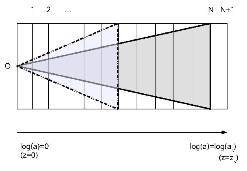
Figure 1: Sketch illustrating the construction of the light cones. A sequence of $N$ lens planes (vertical lines) is used to fill the space between the observer (O) and the sources on the $(N+1)$-th plane. The aperture of the light cone depends on the distance to the last lens plane. At low redshifts, only a small fraction of the lens planes enters the light-cone (dark-gray shaded region). This fraction increases by reducing the redshift of the sources, increasing the aperture of the light cone (light-gray shaded region).

If the size of the light-cone is given by the last lens plane, increasingly smaller fractions of the remaining lens planes will enter the light cone as it approaches $z=0$ ($a=1$, see Fig.1).

3.3 Halo catalogues

Each simulation box contains a large number of dark-matter halos. For our analysis, it is fundamental to know the location of the halos as well as some of their properties, such as their masses and virial radii. Thus, we construct a catalog of halos for each snapshot. The procedure is as follows. We first run a friends-of-friends algorithm to identify the particles belonging to a same group. The chosen linking length is $0.15$ times the mean particle separation. Then, within each group of linked particles, we identify the particle with the smallest value of the gravitational potential. This is taken to be the centre of the halo. Finally, we calculate the matter overdensity in spheres around the halo centre and measure the radius that enclosing an average density equal to the virial density for the adopted cosmological model, $\rho_{\rm vir}=\Delta_{c}(z)\rho_{\rm crit}(z)$, where $\rho_{\rm crit}(z)$ is the critical density of the universe at redshift $z$, and the overdensity $\Delta_{c}(z)$ is calculated as described in Eke et al. (2001).

We end up with a catalogue containing the positions, the virial masses and radii, and the redshifts of all halos in each snapshot. The positions are given in comoving units in the coordinate system of the numerical simulation. They are rotated and shifted in the same way as the particles during the construction of the light-cone. The positions of the halos in the cone are finally projected on the corresponding lens plane.

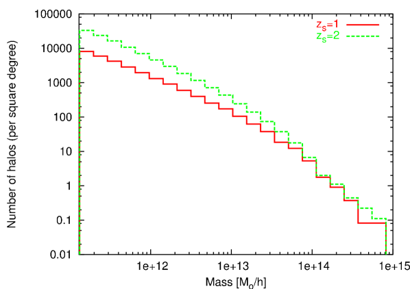
Figure 2: Number of halos per mass bin per square degree. The red and green curves show the halo mass distribution for sources at $z_{\mathrm{s}}=1$ and $z_{\mathrm{s}}=2$, respectively.

In Fig.2, we show the mass functions of the dark-matter halos normalised to one square degree and contained in the light-cones corresponding to $z_{\mathrm{s}}=1$ (solid line) and $z_{\mathrm{s}}=2$ (dashed line). Obviously the light-cones contain a large number of low-mass halos ($\sim 10^{11}-10^{13}\,h^{-1}M_{\odot}$) which are expected to be undetectable through weak lensing. On the other hand, a much lower number of halos with mass $M\gtrsim 10^{13}\,h^{-1}M_{\odot}$ are potential lenses. We note that the numbers of haloes with masses larger than $5\times 10^{13}M_{\odot}$ are approximately equal in both light cones, because such haloes are mainly contained in the low-redshift portion of the volume which is common to both light cones.

We ignore the intracluster gas here because it contributes about one order of magnitude less mass than the dark matter and therefore does not significantly affect the weak-lensing quantities.

3.4 Ray-tracing simulations

The lensing simulations are carried out using standard ray-tracing techniques. Briefly, starting from the observer, we trace a bundle of $2048\times 2048$ light rays through a regular grid covering the first lens plane. Then, we follow the light paths towards the sources, taking the deflections on each lens plane into account.

In order to calculate the deflection angles, we proceed as follows. On each lens plane, the particle positions are interpolated on regular grids of $2048\times 2048$ cells using the triangular-shaped-cloud (TSC) scheme (Hockney & Eastwood, 1988). This allows to avoid sudden discontinuities in the lensing mass distributions, that would lead to anomalous deflections of the light rays (Meneghetti et al., 2000; Hamana & Mellier, 2001). The resulting projected mass maps, $M^{i}_{lm}$, where $l,m=1,...,2048$ and $i=1,...,N$, are then converted into maps of the projected density contrast,

$$\delta^{proj,i}_{lm}=\frac{M^{i}_{lm}}{A_{i}\bar{\rho}}-L_{i}\;,$$ (16)

where $A_{i}$ and $L_{i}$ are the area of the grid cells on the $i$-th plane and the depth of the $i$-th volume used to build the light cone, respectively.

The lensing potential at each grid point, $\psi^{i}_{lm}$, is then calculated using Eq. 9. Owing to the periodic boundary conditions of the density-contrast maps, this is easily solvable using fast-Fourier techniques. Indeed, Eq. 9 becomes linear in Fourier space,

$$\hat{\psi}(\@vec{k})=-3\Omega\left(\frac{H_{0}}{c}\right)^{2}\frac{\hat{\delta}^{proj}(\@vec{k})}{k^{2}}\;,$$ (17)

where $\@vec{k}$ is the wave vector and $\hat{\psi}$ and $\hat{\delta}^{proj}$ are the Fourier transforms of the lensing potential and of the projected density contrast, respectively. Using finite-differencing schemes, we finally obtain maps of the deflection angles on each plane, $\alpha^{i}_{lm}$ (Premadi et al., 1998).

The arrival position of each light ray on the source plane is computed using Eq. 11 which incorporates the deflections on all preceding $N$ lens planes. However, the ray path intercepts the lens plane at arbitrary points, while the deflection angles are known on regular grids. Thus, the deflection angles at the ray position are calculated by bi-linear interpolation of the deflection angle maps.

Again using finite differencing schemes, we employ Eqs. 12 to 15 to obtain maps of the effective convergence and shear.

3.5 Testing the ray-tracing code

We test the reliability of the ray-tracing code by comparing the statistical properties of several ray-tracing simulations with the theoretical expectations for a $\Lambda$CDM cosmology. In these tests, we assume that all source redshifts are $z_{s}=1.5$. For this source redshift, the light cone spans a solid angle of roughly $3.6^{2}\simeq 13$ square degrees on the sky. We perform ray-tracing through 60 different light-cones in total.

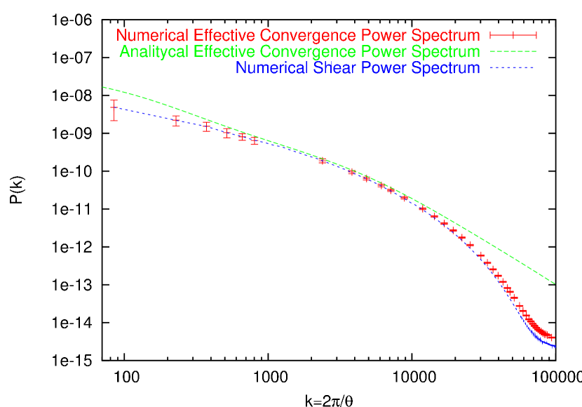
Figure 3: Numerical power spectra of the effective convergence (solid line) and of the shear (dotted line) obtained by averaging over $60$ different light cones corresponding to a solid angle of $\sim 13$ square degrees. The power spectrum expected for a $\Lambda$CDM model with the same cosmological parameters as the simulation is given by the dashed line. The errorbars are shown only for the effective convergence power spectrum, but are of equivalent size for the shear power spectrum.

In Fig. 3, we show the power spectra of the effective convergence and the shear, obtained by averaging over all different realizations of the light-cone. These are given by the solid and by the dotted lines, respectively. The theoretically expected power spectrum is shown as the dashed line. As expected, the convergence and the shear power spectra are equal. We note that they agree with the theoretical expectation over a limited range of wave numbers. Indeed, they deviate from the theoretical power spectrum for $k\lesssim 200$ and for $k\gtrsim 20000$. These two values of the wave vector define the reliability range of these simulations and are both determined by numerical issues. On angular scales $\gtrsim 1^{\circ}$, we miss power because of the small size of the simulation box, while on angular scales smaller than $\lesssim 1^{\prime}$ we suffer from resolution problems due to the finite resolution of the ray and the mass grids.

3.6 Lensing of distant galaxies

Using the effective convergence and shear maps obtained from the ray-tracing simulations, we are now able to apply the lensing distortion to the images of a population of background sources.

In the weak-lensing regime, a sufficiently small source with intrinsic ellipticity $\epsilon_{s}$ is imaged to have an ellipticity

$$\epsilon=\frac{\epsilon_{s}+g}{1+g^{*}\epsilon_{s}}\;,$$ (18)

where $g$ is the complex reduced shear, and the asterisk denotes complex conjugation. We adopt here the standard definition of ellipticity, $\epsilon=\epsilon_{1}+i\epsilon_{2}=(a-b)/(a+b)e^{i2\phi}$, were $a$ and $b$ are the semi-major and the semi-minor axes of an ellipse fitting the object’s surface-brightness distribution. The position angle of the ellipse’s major axis is $\phi$.

The complex reduced shear is defined as

$$g(\@vec{\theta})=\frac{\gamma(\@vec{\theta})}{1-\kappa(\@vec{\theta})}\;.$$ (19)

In the weak-lensing regime, $\kappa\ll 1$ and $\gamma\approx g$. Equation 18 illustrates that the lensing distortion is determined by the reduced shear. Since the background galaxies are expected to be randomly oriented, the expectation value of the intrinsic source ellipticity $\epsilon_{s}$ is assumed to vanish. Thus, the ellipticity induced by lensing can be measured by averaging over a sufficiently large number of galaxies and the expectation value of the ellipticity is equal to the reduced shear, $\langle\epsilon\rangle=g$.

In order to generate a mock catalogue of lensed sources, galaxies are randomly placed and oriented on the source plane. Their intrinsic ellipticities are drawn from the distribution

$$p(|\epsilon_{s}|)=\frac{\exp{|(1-|\epsilon_{s}|^{2})/\sigma_{\epsilon_{s}}^{2}|}}{\pi\sigma_{\epsilon_{s}}^{2}|\exp{(1/\sigma_{\epsilon_{s}}^{2})}-1|},$$ (20)

where $\sigma_{\epsilon_{s}}=0.3$. We assume a background galaxy number density of $n_{g}=30$ arcmin^-2. Observed ellipticities are obtained from Eq. 18 by interpolating the effective convergence and shear at the galaxy positions. This procedure results in catalogues of lensed galaxies for each source redshift chosen, where galaxy positions and ellipticities are stored.

4 Weak lensing estimators

We investigate the performances of three weak-lensing estimators which have been used so far for detecting dark-matter halos through weak lensing. These are the classical aperture mass (Schneider, 1996; Schneider et al., 1998), an optimised version of it (Schirmer et al., 2004), and the recently developed, optimal weak-lensing halo filter (Maturi et al., 2005). More details on these three estimators are given below.

All of them measure the amplitude of the lensing signal $A$ within circular apertures of size $\bar{\theta}$ around a centre $\@vec{\theta}$. Generalisations are possible to apertures of different shapes. In general, $A$ is expressed by a weighted integral of the tangential component of the shear relative to the point $\@vec{\theta}$, $\gamma_{t}$. The weight is provided by a filter function $\Psi$, such that

$$A(\@vec{\theta},\bar{\theta})=\int\mathrm{d}^{2}\theta^{\prime}\gamma_{t}(\@vec{\theta^{\prime}},\@vec{\theta})\Psi(|\@vec{\theta^{\prime}}-\@vec{\theta}|)\;,$$ (21)

and the integral extends over the chosen aperture. The variance of the weak-lensing estimator is given by

$$\sigma^{2}=\frac{1}{(2\pi)^{2}}\int|\hat{\Psi}(\@vec{k})|^{2}P_{N}(k)\mathrm{d}^{2}k,$$ (22)

where $\hat{\Psi}(\@vec{k})$ is the Fourier transform of the filter, and $P_{N}(k)$ the power spectrum of the noise.

4.1 Aperture Mass

The aperture mass was originally proposed by (Schneider, 1996) for measuring the projected mass of dark-matter concentrations via weak lensing. It represents a weighted integral of the convergence,

$$M_{APT}(\@vec{\theta}) = \int\mathrm{d}^{2}\@vec{\theta^{\prime}}\kappa(\@vec{\theta}^{\prime})U(|\@vec{\theta}^{\prime}-\@vec{\theta}|)\;.$$ (23)

The weight function $U(\theta)$ is symmetric if the aperture is chosen to be circular, and it is compensated, i.e.

$$\int_{0}^{\theta}\mathrm{d}\theta^{\prime}\theta^{\prime}U(\theta^{\prime})=0\;.$$ (24)

Since the convergence is not an observable, the aperture mass is more conveniently written as a weighted integral of the tangential shear,

$$M_{APT}(\theta) = \int\mathrm{d}^{2}\@vec{(}\theta^{\prime})\gamma_{t}(\@vec{\theta}^{\prime},\@vec{\theta})\Psi_{APT}(|\@vec{\theta}^{\prime}-\@vec{\theta}|)\;,$$ (25)

where the function $\Psi_{APT}$ is related to the filter function $U$ by the equation

$$\Psi(\theta)=\frac{2}{\theta^{2}}\int_{0}^{\theta}\mathrm{d}\theta^{\prime}\theta^{\prime}U(\theta^{\prime})-U(\theta)\;.$$ (26)

The variance $\sigma^{2}_{M_{APT}}$ of $M_{APT}$ is defined as

$$\sigma^{2}_{M_{APT}}=\frac{\pi\sigma^{2}_{\epsilon_{s}}}{n_{g}}\int_{0}^{\theta}\mathrm{d}\theta^{\prime}\theta^{\prime}\Psi^{2}_{APT}(|\@vec{\theta}^{\prime}-\@vec{\theta}|)\;,$$ (27)

which takes into account the shot noise due to the finite number and the intrinsic ellipticities of the sources (Bartelmann & Schneider, 2001).

The shape of the filter function $\Psi$ is usually chosen to have a compact support and to suppress the halo centre because the lensing measurements are more problematic there. Indeed, the weak-lensing approximation may break down and the cluster galaxies may prevent the ellipticity of background galaxies to be accurately measured.

Schneider et al. (1998) propose the polynomial function

$$\Psi_{APT}=\frac{(1+l)(2+l)}{\pi\theta^{2}_{max}}x^{2}(1-x^{2})^{l}H(1-x)\;,$$ (28)

where $H(x)$ is the Heaviside step function, and $x=\theta/\theta_{max}$ is the radial angular coordinate in units of the radius, $\theta_{max}$, where $\Psi_{APT}$ vanishes. $l$ is a free parameter which is usually set to $l=1$. Note that this filter function was designed especially for measuring cosmic shear. However, several authors have used it for searches for dark matter halos (Erben et al., 2000; Schirmer et al., 2004).

More recently, other filter functions $\Psi$ have been proposed which maximise the signal-to-noise ratio $M_{APT}/\sigma_{M_{APT}}$. Schneider et al. (1998) show that this is the case if $Q$ mimics the shear profile of the lens. For example, Schirmer et al. (2004) propose a fitting formula that approximates the shear profile of a Navarro-Frenk-White (NFW) halo (Navarro et al., 1996). Their filter function is

$$\Psi_{OAPT}(x)=\frac{1}{1+e^{6-150x}+e^{-47+50x}}\frac{\tanh{x/x_{c}}}{x/x_{c}},$$ (29)

where $x_{c}$ is a parameter controlling the shape of the filter (see also Padmanabhan et al., 2003; Hetterscheidt et al., 2005). In the rest of the paper, we will refer to this implementation of the aperture mass as to the “optimised aperture mass”.

Hennawi & Spergel (2005) included the photometric redshifts of background sources, increasing the halo-detection sensitivity at higher redshifts and for smaller masses. Aiming at a comparison of different filters, we neglect this additional information here. We can therefore not apply their tomographic approach, which is based on an NFW fitting formula. They also suggested using a Gaussian profile which found application in actual weak-lensing surveys (see e.g. Miyazaki et al., 2002), but here we focus on the filter proposed by Maturi et al. (2005) whose shape is statistically and physically well motivated.

4.2 Optimal Filter

Maturi et al. (2005) have recently proposed a weak-lensing filter optimised for an unbiased detection of the tangential shear pattern of dark-matter halos. Unlike the optimised aperture mass, the shape of optimal filter is determined not only by the shear profile of the lens, but also by the properties of the noise affecting the weak lensing measurements.

The measured data $D$ is composed of the signal from the lens $S$ and by the noise $N$, and can be written as

$$D(\@vec{\theta})=S(\@vec{\theta})+N(\@vec{\theta})=A\tau(\@vec{\theta})+N(\@vec{\theta})\;,$$ (30)

where $A$ is the total amplitude of the tangential shear and $\tau(\@vec{\theta})$ is its angular shape. The noise $N$ comprises several contributions that can be suitably modeled.

The optimal filter accounts for the noise contributions because it is constructed such as to satisfy two conditions. First, it has to be unbiased, i.e. the average error on the estimate of the lensing amplitude,

$$A_{\rm est}(\@vec{\theta})=\int\mathrm{d}^{2}\theta^{\prime}D(\@vec{\theta}^{\prime})\Psi(|\@vec{\theta}^{\prime}-\@vec{\theta}|)$$ (31)

has to vanish:

$$b\equiv\langle A_{est}-A\rangle=A\left[\int\Psi(\@vec{\theta})\tau(\@vec{\theta})d^{2}\theta-1\right]=0\;.$$ (32)

Second, the noise

$$\sigma^{2}\equiv\langle(A_{est}-A)^{2}\rangle=b^{2}+\frac{1}{(2\pi)^{2}}\int|\hat{\Psi}(\@vec{k})|^{2}P_{N}(k)\mathrm{d}^{2}k$$ (33)

has to be minimal with respect to the signal.

The filter function $\Psi$ satisfying these two conditions is found by combining them with a Lagrangian multiplier $\lambda$. The variation $L=\sigma^{2}+\lambda b$ is carried out, and the filter function $\Psi$ is found by minimising $L$. In Fourier space, the solution of this variational minimisation is

$$\hat{\Psi}_{OPT}(\@vec{k})=\frac{1}{(2\pi)^{2}}\left[\int\frac{|\hat{\tau}(\@vec{k})|^{2}}{P_{N}(k)}\mathrm{d}^{2}k\right]^{-1}\frac{\hat{\tau}(\@vec{k})}{P_{N}(k)}\;,$$ (34)

where the hats denote the Fourier transform. The last equation shows that the shape of the optimal filter $\Psi$ is determined by the shape of the signal, $\tau$, and by the power spectrum of the noise, $P_{N}$.

Maturi et al. (2005) model the signal by assuming that clusters are on average axially symmetric and their shear profile resembles that of an NFW halo (see e.g. Bartelmann, 1996; Wright & Brainerd, 2000; Li & Ostriker, 2002; Meneghetti et al., 2003). Consequently, this filter is optimised for searching for the same halo shape as the optimised aperture mass, even if the filter profile is different.

The noise is assumed to be given by three contributions, namely the noise contributions from the finite number of background sources, the noise from their intrinsic ellipticities and orientations, and the weak-lensing signal due to the large-scale structure of the universe.

The first two sources of noise are characterised by the power spectrum

$$P_{\epsilon}(k)=\frac{1}{2}\frac{\sigma_{\epsilon_{s}}^{2}}{n_{g}}\;,$$ (35)

which depends on the dispersion of the intrinsic ellipticities of the sources, $\sigma_{\epsilon_{s}}$, and on the number density of background galaxies, $n_{g}$.

The statistical properties of the noise due to the lensing signal from the large-scale structure of the universe are described by the power-spectrum of the effective tangential shear. This is related to the power-spectrum of the effective convergence by

$$P_{\gamma}(k)=\frac{1}{2}P_{\kappa}(k)\;.$$ (36)

Thus, the total noise power spectrum is

$$P_{N}(k)=P_{\gamma}(k)+P_{\epsilon}(k)\;,$$ (37)

where $P_{\gamma}$ is determined by the linear theory of structure growth. Using the linear instead of the non-linear power spectrum avoids suppressing a substantial fraction of the signal from the non-linear structures we are searching for. To further reduce any loss of signal in the filtering process, it would be possible to cut $P_{\gamma}$ off at angular scales typical for galaxy clusters. Doing so, we found that this approach has a negligible impact on the final result.

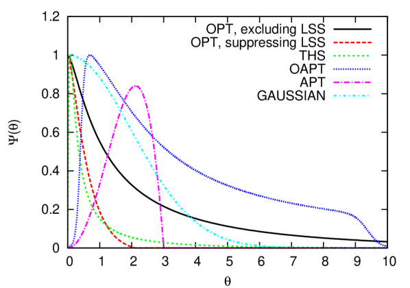
Figure 4: Comparison of the different filter shapes used here and in the literature. The filter scales $r_{\mathrm{s}}$ are those typically used in the literature. Note how the optimal filter (black solid curve) shrinks when the linear matter power spectrum is used to suppress the LSS contribution (red dashed curve). Interestingly, Hennawi & Spergel (2005) found experimentally that the truncated NFW-shaped filter (cyan curve) performs best when scaled to the green curve (THS), which approximates the optimal filter (OPT, red curve) almost precisely. The advantage of the optimal compared to the other filters is that its shape and scale are physically and statistically well motivated such that it needs not be experimentally rescaled.

In Fig. 4, we compare the filters studied here and in the literature. They are scaled in such a way as they are typically discussed or applied in the literature (see also the figure legend and caption for more detail). At first sight, the scales are surprisingly different. When the optimal filter is constructed including the linear matter power spectrum such as to best suppress the LSS contribution, it shrinks considerably. It is reassuring that the truncated NFW-shaped filter (THS) proposed and heuristically scaled by Hennawi & Spergel (2005) to yield best results almost exactly reproduces the optimal filter. They are therefore expected to perform similarly well. The optimised aperture-mass filter (OAPT) also peaks at fairly small angular scales, but shows the long tail typical for the NFW profile. The aperture mass has its maximum at comparatively large radii, explaining why the APT filter yields results most severely affected by the LSS.

5 Results

5.1 Signal-to-noise maps

We now use the above-mentioned weak-lensing estimators to analyse our mock catalogues of lensed galaxies.

In practice, the integral in Eq. 21 is replaced by a sum over galaxy images. Moreover, since the ellipticity $\epsilon$ is an estimator for $\gamma$, we can write

$$A_{est}(\@vec{\theta})=\frac{1}{n_{g}}\sum_{i}\epsilon_{ti}(\@vec{\theta_{i}})\Psi(|\@vec{\theta_{i}}-\@vec{\theta}|)\;,$$ (38)

where $\epsilon_{ti}(\@vec{\theta_{i}})$ is the tangential component of the observed ellipticity of the galaxy at $\@vec{\theta}_{i}$, with respect to the point $\@vec{\theta}$. Similarly, the noise estimate in $A_{est}$ is given by

$$\sigma^{2}(A_{est})(\@vec{\theta})=\frac{1}{2n_{g}^{2}}\sum_{i}|\epsilon_{i}(\@vec{\theta_{i}})|^{2}\Psi^{2}(|\@vec{\theta_{i}}-\@vec{\theta}|).$$ (39)

Computing $A_{est}$ and $\sigma^{2}(A_{est})$ on a grid covering our simulated sky, we produce maps of the signal-to-noise ratio for all the weak lensing estimators. We use three different filter sizes for each estimator in order to test the stability of the results achieved. These have been calibrated among the different filters to allow the optimal detection of similar objects. For the optimal filter, we used sizes of $1^{\prime}$, $2^{\prime}$ and $4^{\prime}$. These correspond to $2.75^{\prime}$, $5.5^{\prime}$ and $11^{\prime}$ for the aperture mass, for the optimised aperture mass we used the values $5^{\prime}$, $10^{\prime}$ and $20^{\prime}$ that are widely used in literature.

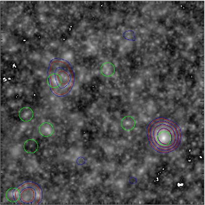
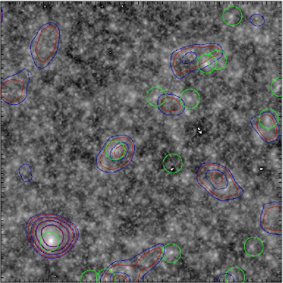
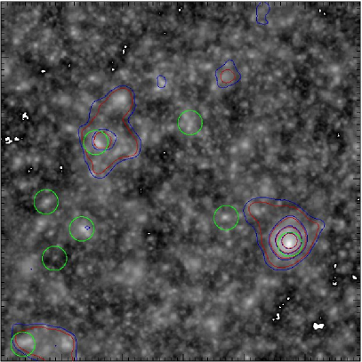
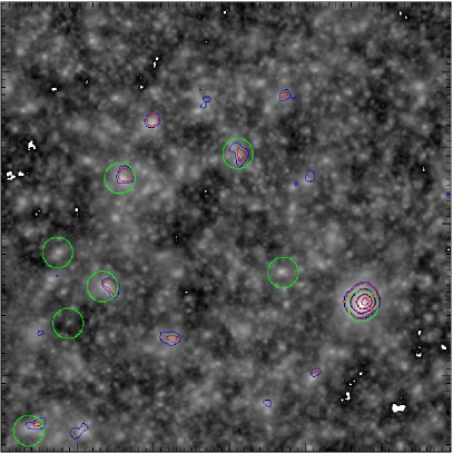
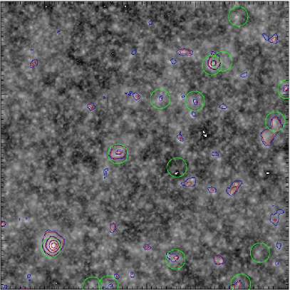
Figure 5: Maps of the effective convergence for sources at redshift $z_{s}=1$ (left panels) and $z_{s}=2$ (right panels) for a region of simulated sky. Superimposed are the iso-contours of the signal-to-noise ratio of the weak-lensing signal measured with three estimators, namely the APT (top panels), the OAPT (middle panels) and the OPT (bottom panels). The iso-contours start from $S/N=4$ with a step of 3. The positions of the halos contained in the field-of-view having mass $M>7\times 10^{13}h^{-1}M_{\odot}$ are identified by circles. The filter sizes are $11^{\prime}$, $20^{\prime}$ and $4^{\prime}$ for the APT, the OAPT and the OPT, respectively.

In Fig. 5 we show examples of the signal-to-noise iso-contours of the weak lensing signal, superimposed on the corresponding effective convergence maps of the underlying projected matter distribution for sources at redshift $z_{s}=1$ (left panels) and $z_{s}=2$ (right panels). The iso-contours start at $S/N=4$ with a step of 3. From top to bottom, the maps refer to the results obtained using the aperture mass (APT), the optimised aperture mass (OAPT) and the optimal filter (OPT) with sizes of $11^{\prime}$, $20^{\prime}$ and $4^{\prime}$, respectively. The circles identify halos with mass $M\geq 7\times 10^{14}h^{-1}M_{\odot}$ present in the field-of-view. The side length of each map is one degree.

The images show that, for sources at high redshift, all three estimators can successfully detect the weak-lensing signal from clusters in the mass range considered. However, spurious detections, corresponding to high signal-to-noise peaks not associated with any halo, also appear. Their significance and spatial extent is larger in the case of the APT and the OAPT filters. This confirms the results of Maturi et al. (2005).

For lower-redshift sources, the OPT detects five out of the seven halos present in the field, while the APT and the OAPT detect substantially fewer halos. For the OPT, the number of spurious detections is roughly the same or slightly smaller than for sources at higher redshift, while it is strongly reduced for the APT and the OAPT. The natural explanation of these results is that the detections with the APT and the OAPT are strongly contaminated by the noise from large-scale structure lensing, which becomes increasingly important for sources at higher redshift. This noise is efficiently filtered out by the OPT.

5.2 True and spurious detections

In the following, we call a detection a group of pixels in the $S/N$ maps above a threshold $S/N$ ratio. Its position in the sky is given by the most significant pixel, i.e. that with the highest $S/N$ ratio.

A true detection is obviously a detection that can be associated with some halo in the simulation. A spurious detection is instead mimicked by noise, in particular by cosmic structures aligned along the line-of-sight.

The association between weak-lensing detections and cluster halos is established by comparing their projected positions on the sky. This causes a problem, because the simulation boxes contain plenty of low-mass halos that are not individually detectable through lensing but happen to be projected near the line-of-sight towards a detection. Thus, spurious detections could easily be erroneously associated with these low-mass halos on the basis of the projected position only.

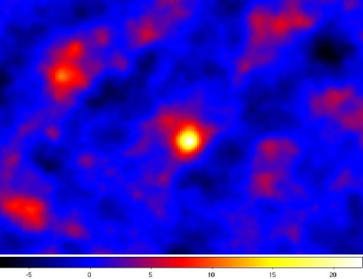
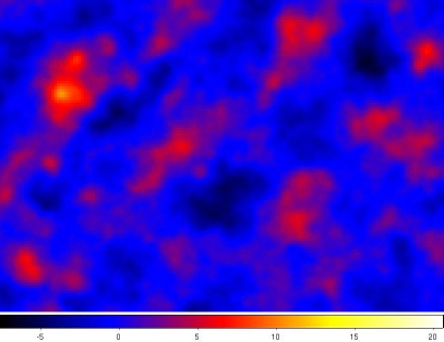
Figure 6: Map of the $S/N$ ratio corresponding to a region of 3 square degrees. The map was created using the OAPT estimator, with a filter scale of $20^{\prime}$ and assuming a source redshift of $z_{s}=1$. The left panel shows the $S/N$ ratio map including all lens planes, while the right panel shows the same map obtained after removing the lens plane containing the cluster responsible for the highest $S/N$ peak in the left panel.

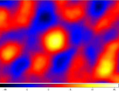
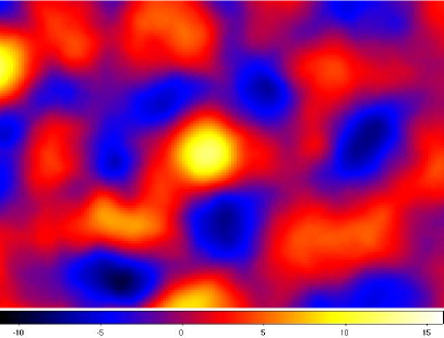
Figure 7: Maps of the $S/N$ ratio corresponding to a region of 3 square degrees. The maps were created with the APT estimator, with a filter scale of $11^{\prime}$ and assuming a source redshift of $z_{s}=2$. The left panel shows a true detection, while the right panel shows a spurious detection.

As pointed out earlier, we describe the lensing effect of the matter contained in the light cone with a stack of lens planes. Cluster halos are localised structures, i.e. their signal originates from a single lens plane. Thus, any detection should disappear when its plane is removed from the stack. Conversely, spurious detections are not caused by localised structures and should remain even after removing an individual lens plane. This is illustrated by the $S/N$ maps shown in Fig. 6. The map in the left panel includes all lens planes, while one plane was removed for the right panel. Both maps were obtained with the OAPT estimator with a filter size of $20^{\prime}$ and a source redshift of $z_{s}=1$. Clearly, the highest peak in the left panel, which is in fact produced by a massive halo, disappears in the right panel, after removing the lens plane from the stack which contains the halo. All other features in the left upper map remain unchanged.

This allows us to verify the reliability of detections associated with some halo in the catalogue. For each positive match, we estimate the lensing signal before and after removing the plane containing the candidate lensing halo from the lens-plane stack. If this causes a significant decrease in the $S/N$ ratio, we classify the detection as true, and otherwise as spurious. We estimate through several checks of detections associated to the halos that $S/N$ fluctuations of order $25\%$ of the initial value are possible due to different properties of the noise. Thus, we set this limit as our threshold for discriminating between true and spurious detections.

This method also shows its power when pixels identifying a true detection are compared with pixels associated to a spurious detection. This is shown in Fig. 7. The map in the left panel represents a true detections, while the map on the right panel shows a spurious detections. The maps refer to different regions of a $S/N$ map created with the APT estimator with a filter size of $11^{\prime}$ and a source redshift of $z_{s}=2$. As it is clearly seen, it is impossible a priori to distinguish which of the two is spurious.

5.3 Statistical analysis of the detections

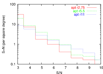
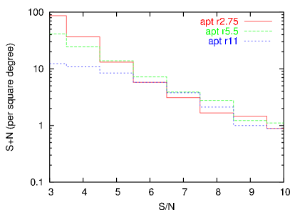
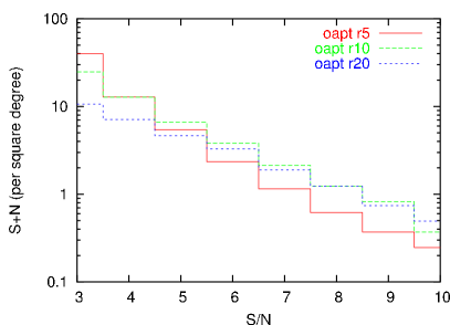
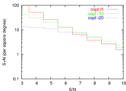
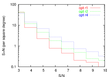
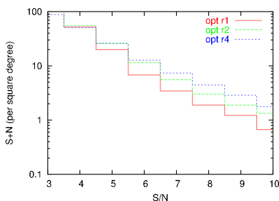
Figure 8: Number of detections as a function of the $S/N$ ratio obtained by using the APT (top panels), the OAPT (middle panels) and the $OPT$ weak lensing estimators. Results for sources at redshift $z_{s}=1$ and $z_{s}=2$ are shown in the left and in the right panels, respectively. Different line styles refer to three different filter sizes. For the OPT, these are $1^{\prime}$, $2^{\prime}$ and $4^{\prime}$. They correspond to $2.75^{\prime}$, $5.5^{\prime}$, and $11^{\prime}$ for the APT and to $5^{\prime}$, $10^{\prime}$ and $20^{\prime}$ for the OAPT.

In Fig. 8, we show the number of detections per square degree in $S/N$ ratio bins, ignoring for now the distinction between true and spurious detections. Left and right panels refer to simulations with sources at redshifts $z_{s}=1$ and $z_{s}=2$, respectively. From top to bottom, we show the results for the APT, the OAPT and the OPT estimators. In each panel, we use solid, dashed and dotted lines to display the histograms corresponding to increasing filter sizes.

For low source redshifts and small filter sizes, the APT and the OPT estimators lead to similar numbers of detections. Instead, for the OAPT, the number of detections is larger by up to a factor of two for $S/N\gtrsim 4$. Increasing the filter size, the number of detections generally increases for all estimators, especially for large $S/N$ ratios and in particular for the OPT.

We notice, however, that for small $S/N$ ratios, larger filters produce lower numbers of detections for the APT and for the OAPT. This behaviour is more evident for sources at higher redshifts. For example, we find that the number of detections with $S/N=4$ drops by a factor of $4$ for the APT and by a factor of $\sim 7$ for the OAPT, when increasing the filter size from $2.5^{\prime}$ to $11^{\prime}$ and from $5^{\prime}$ to $20^{\prime}$, respectively. Increasing the filter size, the weak-lensing signal is estimated by averaging over more background galaxies. Thus, high $S/N$ peaks are smoothed, and some detections may be suppressed. This affects mainly the detections with the APT and the OAPT filters. On the other hand, the OPT filter shrinks in response to the noise introduced by the large scale structure, largely reducing this effect compared to the APT and the OAPT.

The fractions of spurious detections are shown in Fig. 9. Clearly, the OPT estimator performs better than the APT and the OAPT. For sources at redshift $z_{s}=1$ and $z_{s}=2$, the fraction of spurious detections with the OPT is less than $20\%$ and $30\%$ at $S/N\sim 4$. This fraction decreases below $10\%$ for $S/N\gtrsim 5$ and drops rapidly to zero for higher $S/N$ ratios. Results are very stable against changes in the filter size. Conversely, the APT and the OAPT estimators yield similarly low fractions of false detections only for the smallest apertures.

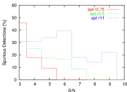
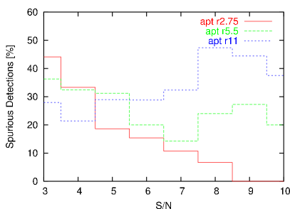
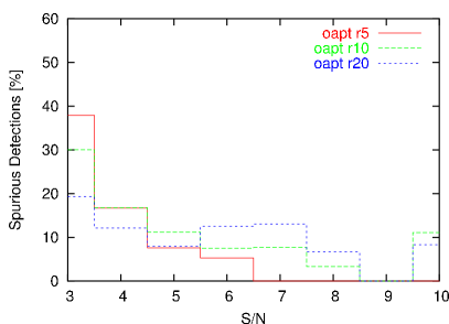
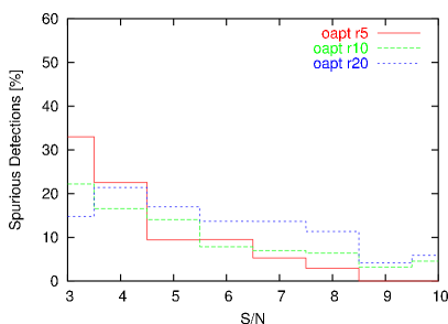
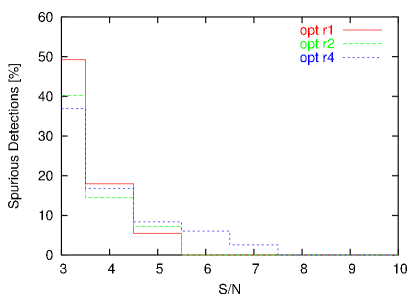
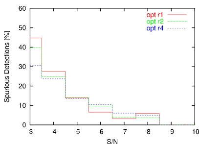
Figure 9: Fraction of spurious detections as a function of the $S/N$ ratio obtained by using the APT (top panels), the OAPT (middle panels) and the $OPT$ weak-lensing estimators. Results for sources at redshift $z_{s}=1$ and $z_{s}$=2 are shown in the left and the right panels, respectively. Different line styles refer to three filter sizes. For the OPT these are $1^{\prime}$, $2^{\prime}$ and $4^{\prime}$. They correspond to $2.75^{\prime}$, $5.5^{\prime}$, and $11^{\prime}$ for the APT and to $5^{\prime}$, $10^{\prime}$ and $20^{\prime}$ for the OAPT.

Depending on the filter shape, its size and on the source redshift, a $S/N$ threshold can be defined above which there are no spurious detections and thus all detections are reliable. For the OPT estimator, this minimal signal-to-noise ratio is between $5$ and $8$. It increases above $10$ for the APT and the OAPT estimators if large filter sizes are used. These results agree with the results of Maturi et al. (2005), using numerical simulations, and of Maturi et al. (2006), regarding the analysis of the GaBoDS survey.

Here, we studied the contaminations by the LSS, the intrinsic ellipticity and the finite number of background galaxies all together. To gain an idea which of those is the main source for spurious detections, we used the APT with $r_{s}=11^{\prime}$ to analyse a catalog of galaxies with intrinsic ellipticities set to zero. In this case, the S/N ratio is enhanced by a factor of four uniformly across the whole field, but the morphology of the map is not affected. The same should apply to the finite number of background sources. We thus conclude that the main source of spurious detections is the LSS, as already noted by Reblinsky & Bartelmann (1999) and White et al. (2002).

5.4 Sensitivity

We shall now quantify which halo masses the weak-lensing estimators are sensitive to.

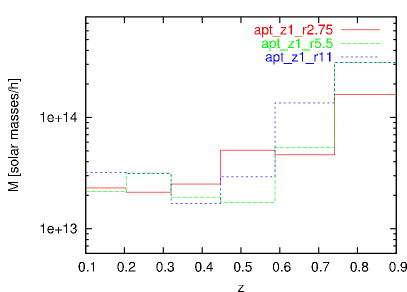
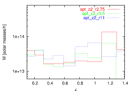
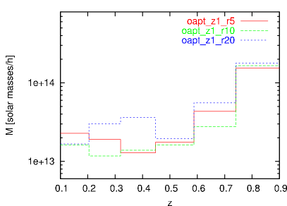
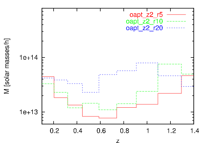
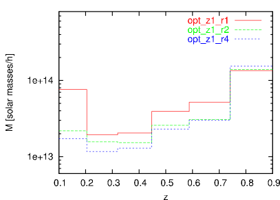
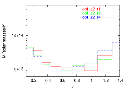
Figure 10: Minimum detected halo mass as a function of redshift for the APT (top panels), the OAPT (middle panels) and for the OPT (bottom panels) estimators. Results for sources at redshift $z_{s}=1$ and $z_{s}$=2 are shown in the left and in the right panels, respectively. Different line styles refer to three filter sizes. For the OPT, these are $1^{\prime}$, $2^{\prime}$ and $4^{\prime}$. They correspond to $2.75^{\prime}$, $5.5^{\prime}$, and $11^{\prime}$ for the APT and to $5^{\prime}$, $10^{\prime}$ and $20^{\prime}$ for the OAPT. Results for each redshift bin are averaged between two planes.

Figure 10 shows the lowest mass detected in each redshift bin. This is defined as the mean mass of the ten least massive halos detected in this bin. Again, results are displayed for all weak-lensing estimators, for different filter sizes and for two source redshifts.

We note that the performance of the three filters is very similar for sources at redshift $z_{s}=1$ (left panels). The OPT (bottom panels) is only slightly more efficient in detecting low-mass halos than the APT (top panels) and the OAPT (middle panels). The minimal mass detected depends on the lens redshift. All filters allow the detection of low-mass halos more efficiently if these are at redshifts between $0.2$ and $0.5$, i.e. at intermediate distances between the observer and the sources. This obviously reflects the dependence of the geometrical lensing strength on the angular-diameter distances between the observer and the lens, the lens and the sources, and the observer and the sources. The lowest detected masses fall within $\sim 10^{13}h^{-1}M_{\odot}$ and $\sim 10^{14}h^{-1}M_{\odot}$ for the OPT estimator.

For sources at higher redshift, the region of best filter performance shifts to higher lens redshift, between $0.5$ and $0.8$. We note that due to the increasing importance of lensing by large-scale structures, the differences between the estimators are more significant. The OPT estimator allows the detection of halos with masses as low as $\lesssim 10^{13}h^{-1}M_{\odot}$, almost independently of the filter size. Similar masses are detected with the OAPT only for the smallest apertures. With the APT and the OAPT, the results are indeed much more sensitive to the filter size than with the OPT. Increasing the filter size pushes the detectability limit to larger masses. Again, as discussed in Sect. 5.3, this is due to the fact that the signal from low-mass halos is smeared out by averaging over an increasing number of galaxies entering the aperture. For example, the minimal mass detected with the OAPT filter at $z\sim 0.8$ changes by one order of magnitude by varying the filter scale from $5^{\prime}$ to $20^{\prime}$.

5.5 Completeness

We now discuss the completeness of a synthetic halo catalogue selected by weak lensing.

Figure 11 shows the fraction of halos contained in the light cone that are detected with different weak lensing estimators as a function of their mass. Again, we find that the OPT filter yields the most stable results with respect to changes in the filter size. This is particularly evident for sources at redshift $z_{s}=2$ (right panels), while the differences are smaller for $z_{s}=1$ (left panels). As discussed earlier, the APT and the OAPT become less efficient in detecting low-mass halos when the filter size is increased.

For the OPT estimator, the completeness reaches $100\%$ for masses $M\gtrsim 3\times 10^{14}h^{-1}M_{\odot}$ and $M\gtrsim 2\times 10^{14}h^{-1}M_{\odot}$ for sources at redshift $z_{s}=1$ and $z_{s}=2$, respectively. For lower masses, the completeness drops quickly, reaching $\sim 50\%$ already at $M\sim 2\times 10^{14}h^{-1}M_{\odot}$ for low-redshift sources, and at $M\sim 7\times 10^{13}h^{-1}M_{\odot}$ for high-redshift sources. Similar results are obtained with the APT and the OAPT only for small apertures.

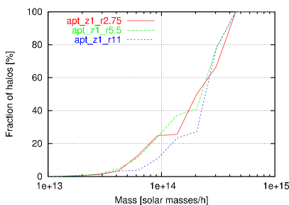
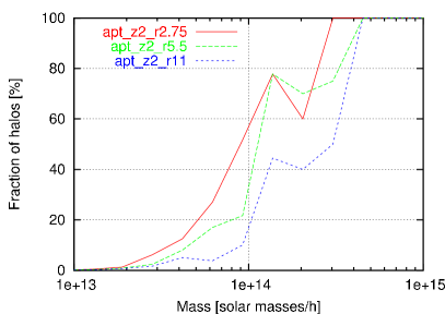
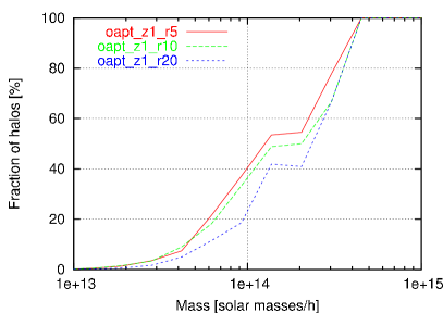
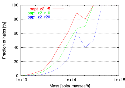
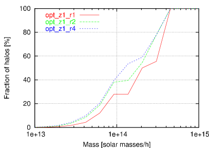
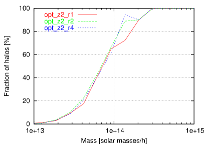
Figure 11: Fraction of detections as a function of the halo mass. Each plot contains results obtained with the three filter radii used in this work. The panels on the left show curves for sources at $z_{s}=1$, the panels on the right for sources at $z_{s}=2$. From top to bottom we have the APT, the OAPT and the OPT.

Figure 11 gives a global view of the halos detected, regardless of the their redshift. In Fig. 12, we selected three mass bins ($M=2.5\times 10^{13}M_{\odot}/h$, $M=5\times 10^{13}M_{\odot}/h$, $M=10^{14}M_{\odot}/h$) and determined the fraction of halos detected as a function of the redshift.

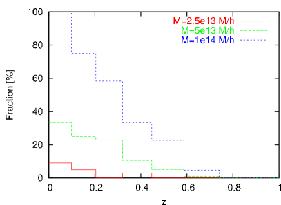
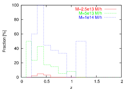
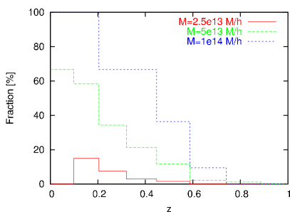
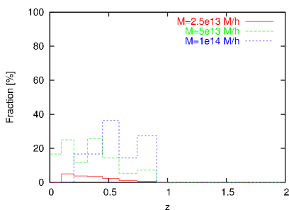
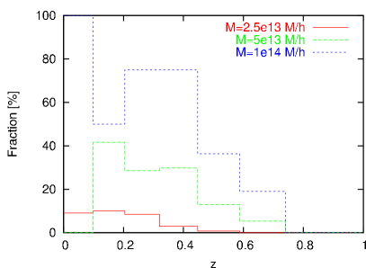
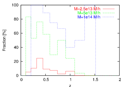
Figure 12: Fraction of halo detections with the APT, OAPT and OPT (from top to bottom) as a function of the halo redshift for three particular masses. The red line corresponds to a mass of $M=2.5\times 10^{13}M_{\odot}/h$, the green line to $M=5\times 10^{13}M_{\odot}/h$ and the blue line to $M=10^{14}M_{\odot}/h$. The panels on the left show the results for sources at $z_{s}=1$ and those on the right for sources at $z_{s}=2$. From top to bottom, the filter radii are $r=5.5^{\prime}$ (for APT), $r=10^{\prime}$ (for OAPT) and $r=2^{\prime}$ (for OPT). Results for each redshift bin are averaged between two planes.

To reduce the noise, we binned together two lens planes as in Fig. 10. Yet, the results are still noisy, there is much variation for all the filters when the filter radius is changed, and the performance of the filters is quite similar in this respect. We see from the figure that the detected halos are preferentially located at low and moderate redshifts, due, as already said, to the geometry of the lensing strength.

5.6 Comparison with the peak statistics

The peak statistic counts peaks in convergence maps, e.g. obtained with the Kaiser-Squires inversion (see Kaiser & Squires, 1993; Kaiser, Squires & Broadhurst, 1995), usually smoothed with a Gaussian kernel. Even though they used a different set of numerical simulations, we can safely compare our results with the peak-statistic analysis by Hamana et al. (2004), whose Gaussian kernel has a FWHM of 1 arcmin.

Fixing a detection threshold of $S/N>4$ ($5$), Hamana et al. (2004) found $N\approx 6$ $(2.5)$ detections per square degree, $60\%$ $(76\%)$ of which correspond to real haloes with masses larger than $10^{13}\,h^{-1}M_{\odot}$. In our simulations, with the same S/N threshold and the optimal filter by Maturi et al. (2005), we found $N\approx 10$ ($7$), with an efficiency in detecting real haloes of $85\%$ ($95\%$). For halos with masses $M>2\times 10^{14}\,h^{-1}M_{\odot}$ ($M\approx 1\times 10^{14}\,h^{-1}M_{\odot}$), the Hamana et al. (2004) sample is complete at the $70\%$ ($50\%$) level, which is virtually identical to the completeness of $70\%$ ($50-60\%$) achieved with the optimal filter.

6 Comparison with observations

The results outlined above show interesting differences between the performances of the filter functions. The discrepancies are particularly significant for high-redshift sources, indicating that the noise due to the LSS should become important only for deep observations. We can now attempt a quick comparison of our simulations with the observational results existing in the literature. In particular, we focus here on the searches for dark matter concentrations in the GaBoDS survey (Schirmer et al., 2003; Maturi et al., 2006).

To this goal, we perform a new set of ray-tracing simulations, where a realistic redshift distribution of the sources is assumed. In particular, we draw the sources from the probability distribution function

$$P(z)=N\exp[-(z/z_{0})^{\beta}]\;,$$ (40)

where $N$ is chosen such that

$$\int_{0}^{\infty}P(z)\mathrm{d}z=1\;.$$ (41)

We adapt $P(z)$ to the redshift distribution of the sources in the GaBoDS survey by setting $z_{0}=0.4$ and $\beta=1.5$ (Schirmer et al., 2003). In order to mimic the number density of galaxies in the GaBoDS observations, we assume $n_{g}=10\,\mathrm{arcmin}^{-1}$.

By repeating the same analysis outlined above, we find results that are compatible with the results of Maturi et al. (2006). In particular, the number of detections with $S/N=3.5$ per square degree in our GaBoDS simulations (in GaBoDS data) are $\simeq 5$ ($\simeq 4$) for the OPT with $r=2^{\prime}$, $\simeq 3$ ($\simeq 3$) for the OAPT with $r=10^{\prime}$ and $\simeq 1.5$ ($\simeq 2$) for the APT with $r=5.5^{\prime}$ ($r=4^{\prime}$) respectively. A comparison between the detections with different weak lensing estimators is shown in Fig. 13.

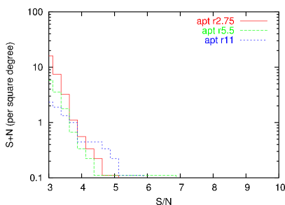
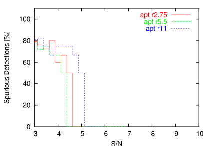
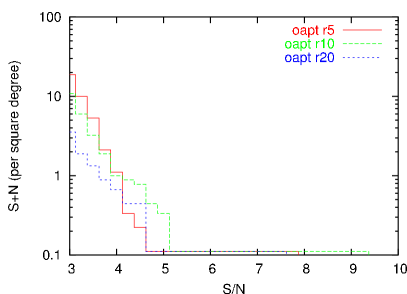
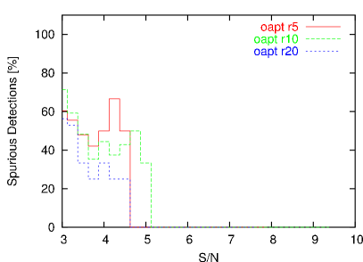
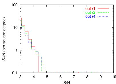
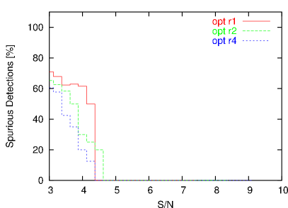
Figure 13: Total number of detections per square degree (left panels) and fraction of spurious detections (right panels) for sources distributed in redshift as in the GaBoDS survey (Schirmer et al., 2003). From top to bottom, we show the APT (for $r=2.75^{\prime}$, $r=5.5^{\prime}$ and $r=11^{\prime}$), the OAPT ($r=5^{\prime}$, $r=10^{\prime}$ and $r=20^{\prime}$) and the OPT ($r=1^{\prime}$, $r=2^{\prime}$ and $r=4^{\prime}$).

The fraction of spurious detections is large for all filters, but it is generally smaller for the OAPT and the OPT. As expected, the OAPT and the OPT estimators have similar performances, because of the small density of background galaxies. Indeed, the noise due to the intrinsic shape of the sources is dominant with respect to that due to the LSS and thus, according to Equation (34), the two filter functions have a very similar shape.

A more detailed statistical analysis, including simulations representative of different current surveys (both ground- and space-based), will be presented in a future paper.

7 Conclusions

We studied the performance of dark-matter halo detection with three different linear filters for their weak-lensing signal, the aperture mass (APT), the optimised aperture mass (OAPT), and a filter optimised for distinguishing halo signals from spurious signals caused by the large-scale structure (OPT). In particular, we addressed the questions how the halo selection function depends on mass and redshift, how the number of detected halos and of spurious detections depends on parameters of the observation, and how the filters compare.

To this end, we used a large $N$-body simulation, identified the halos in it and used multiple lens-plane theory to determine the lensing properties along a fine grid of light rays traced within a cone from the observer to the source redshift. Halos were then detected as peaks in the filtered cosmic-shear maps. By comparison with the known halo catalog, spurious peaks could be distinguished from those caused by real halos.

Our main results are as follows:

• We confirm that among those tested, the optimised filter (OPT) proposed by Maturi et al. (2005) performs best in the sense that its results are least sensitive to changes in the angular filter scale, it produces the least number of spurious detections, and it has the lowest mass limit for halo detection (cf. Figs. 9, 10 and 11).

• With the OPT filter, the fraction of spurious detections is typically $\lesssim 10\%$ for a signal-to-noise threshold of $S/N\approx 5$. It increases with source redshift due to the larger contamination by large-scale structure lensing (cf. Fig. 9).

• The number of halos detected per square degree by the OPT filter with $S/N\gtrsim 5$ is a few if the sources are at redshift $z_{s}=1$, and $\sim 20$ for $z_{s}=2$ (cf. Fig. 8).

• The minimum detectable halo mass starts at a few times $10^{13}\,h^{-1}\,M_{\odot}$ at redshifts $\sim 0.1$, drops to $\sim 10^{13}h^{-1}\,M_{\odot}$ near the optimal lensing redshift and increases towards $\sim 10^{14}h^{-1}\,M_{\odot}$ approaching the source redshift (cf. Fig. 10).

• The fraction of halos detected reaches $\sim 50\%$ at $\sim 2\times 10^{14}h^{-1}\,M_{\odot}$ and $100\%$ at $\sim 4.5\times 10^{14}h^{-1}\,M_{\odot}$ with sources at $z_{s}=1$. With more distant sources at $z_{s}=2$, half of the halos with $\sim 7\times 10^{13}h^{-1}\,M_{\odot}$ are found, and all halos above $\sim 3\times 10^{14}h^{-1}\,M_{\odot}$ (cf. Fig. 11).

• Adapting parameters to the GaBoDS survey (Schirmer et al., 2003), and distributing sources in redshift, our simulation yields a number of significant detections per square degree which is in good agreement with what was found applying the OPT filter to the real GaBoDS data (Maturi et al., 2006).

Thus, the OPT filter, optimised for suppressing contaminations by large-scale structures, allows the reliable detection of dark-matter halos with masses exceeding a few times $10^{13}\,h^{-1}\,M_{\odot}$ with a low contamination by spurious detections.