Magnetic-Optical Filter

Abstract

Magnetic-Optical Filter (MOF) is an instrument suited for high precision spectral measurments for its peculiar characteristics. It is employed in Astronomy and in the field of the telecommunications (it is called FADOF there). In this brief paper we summarize its fundamental structure and functioning.

Magnetic-Optical Filter (MOF) was developed in the 60’s in Rome by professor Cacciani. Its more important features are good spectral resolution, high transmission, high field of view and an absolute spectral reference. In Naples, at the Osservatorio Astronomico di Capodimonte (OAC), it’s utilized in the VAMOS (Velocity And Magnetic Observations of the Sun) project, whose aim is to measure Solar surface’s velocity field and magnetic field along the line of sight. Moreover the high signal-to-noise ratio of the MOF permits its use in the telecommunications too (here it’s called FADOF, Faraday Anomalous Dispersion Optical Filter).

In the VAMOS instrument, MOF consists of a potassium vapours cell with a magnetic field (about 1400 G) along its optic axis, interposed between two crossed linear polarizers. In order to understand how this works, we have to recall the Zeeman effect. Let’s consider the atomic transition from the level with $l=1$ to that with $l=0$ (where $l$ is the angular momentum quantum number): in absence of magnetic field, there is only an emission line. If we are in presence of a magnetic field, the degeneration of the level with $l=1$ is removed bringing to three different states with three different values of the atomic quantum number $m$ (magnetic moment quantum number) and we can see no more one emission line, but three emission lines characterized by different states of polarization. In fact two of these emission lines are circularly polarized, respectively right-handed ($\sigma^{+}$) and left-handed ($\sigma^{-}$), around the magnetic field direction, the other ($\pi$) is linearly polarized along the magnetic field, so, when we observe along this direction (it’s our case) we can’t see this last component. MOF is based on two effects: the Righi Effect and the Macaluso-Corbino Effect. Righi Effect is Zeeman effect in absorption: solar light (not polarized) arrives on the first polarizer which transforms it in linearly polarized light (let’s recall that linearly polarized light can be viewed as half right circularly polarized and half left circularly polarized); then the cell absorbs half of the light intensity at $\sigma^{+}$ and $\sigma^{-}$ wavelengths and the second polarizer cuts half of the light intensity at $\sigma^{+}$ and $\sigma^{-}$ wavelengths and cuts totally the other wavelengths. So, at the output, we should see only two peaks at the Zeeman wavelengths, but the net output of the filter is characterized by the presence of the Macaluso-Corbino Effect, too. This consists in a rotation of the polarization plane caused by a difference in refraction index values at the two Zeeman wavelengths in the cell. Higher is the temperature of the cell, stronger is the Macaluso-Corbino Effect which shows itself as two additional symmetric peaks, the distance between which increases linearly with temperature (in the range considered in our work). In figure 1 we report the transmission profile in which is visible the sum of the two effects.

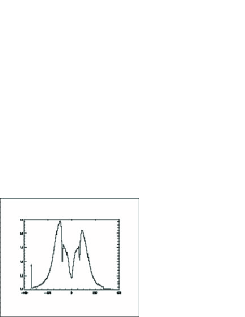
Figure 1: Transmission profile of MOF at the temperature of 160^oC. The Righi and Macaluso-Corbino effects are visible in the figure; the first effect manifests itself as the two plateaux between the two external peaks of the Macaluso Corbino Effect

To calibrate in wavelength the profiles we measured by a laser diode system, we used the Zeeman effect. In fact, by using the laser diode, we obtained profiles in function of the voltage applied to the laser cavity. Because we knew the difference $\Delta\lambda$ between the two Zeeman wavelengths (it’s given by the product $4.67\times 10^{-13}\lambda^{2}{g}\mathbf{B}$, $\lambda$ is the unperturbed wavelength (in Angstrom), $g$ a factor containing the Lande’ factor and $\mathbf{B}$ is the magnetic field’s intensity), we could obtain profiles in function of the wavelength. Profiles utilized in the calibration were that obtained at lower temperatures ($70^{\circ}C$, $80^{\circ}C$, $90^{\circ}C$), where Zeeman lines were easier to detect.

MOF and Wing Selector (WS) form the basis of the VAMOS instrument. WS’ role is to select only one of the two MOF output lines. It’s composed by a quarter-wave plate and a cell analogous to MOF’s cell. If the plate’s transmission axis forms with the optic axis an angle of 45 degrees, light’s polarization becomes right circular and so the cell cuts the $\sigma^{+}$ component, while leaves the $\sigma^{-}$ one to pass; if the plate’s transmission axis forms with the optic axis an angle of -45 degrees, we have the opposite situation and only the $\sigma^{-}$ component passes.