Studying stellar populations at high spectral resolution

Abstract

I describe very briefly the new libraries of empirical spectra of stars covering wide ranges of values of the atmospheric parameters T_eff, log g, [Fe/H], as well as spectral type, that have become available in the recent past, among them the HNGSL, MILES, UVES-POP, ELODIE, and the IndoUS libraries. I show the results of using the IndoUS and the HNGSL libraries, as well as an atlas of theoretical model atmospheres, to build population synthesis models. These libraries are complementary in spectral resolution and wavelength coverage, and will prove extremely useful to describe spectral features expected in galaxy spectra from the NUV to the NIR. The fits to observed galaxy spectra using simple and composite stellar population models are discussed.

C.I.D.A., Apartado Postal 264, Mérida 5101-A, Venezuela

1. Introduction

Bruzual & Charlot (2003), hereafter BC03, have examined in detail the advantages of using intermediate resolution stellar spectra in population synthesis and galaxy evolution models. In these models BC03 use the STELIB library compiled by Le Borgne et al. (2003). This library contains observed spectra of 249 stars in a wide range of metallicities in the wavelength range from 3200 Å to 9500 Å at a resolution of 3 Å FWHM (corresponding to a median resolving power of $\lambda/\Delta\lambda\approx 2000$), with a sampling interval of 1 Å and a signal-to-noise ratio of typically 50 per pixel. The BC03 models reproduce in detail typical galaxy spectra extracted from the SDSS Early Data Release, e.g., Stoughton et al. (2002). From these spectral fits one can constrain physical parameters such as the star formation history, metallicity, and dust content of galaxies, e.g., Heavens et al. (2004); Cid-Fernandes et al. (2005); Mateu, Magris, & Bruzual (2005). The medium resolution BC03 models also enable accurate studies of absorption-line strengths in galaxies containing stars over the full range of ages and can reproduce simultaneously the observed strengths of those Lick indices that do not depend strongly on elemental abundance ratios, provided that the observed velocity dispersion of the galaxies is accounted for properly, and offer the possibility to explore new indices over the full optical range of the STELIB atlas, i.e. 3200 Å to 9500 Å. To extend the spectral coverage in the models beyond these limits, BC03 recur to other libraries. For solar metallicity models, the Pickles (1998) library can be used to extend the STELIB spectral coverage down to 1150 Å in the UV end and up to 2.5 $\mu$m at the red end, with a sampling interval of 5 Å pixel^-1 and a median resolving power of ($\lambda/\Delta\lambda\approx 500$). The UV spectra in the Pickles (1998) atlas are based on $IUE$ spectra of bright stars. At all metallicities the BC03 models are extended down to 91 Å in the UV side and up to 160 $\mu$m at the other end using the theoretical model atmospheres included in the BaSeL series of libraries compiled by Lejeune, Cuisinier, & Buser (1997, 1998), and Westera et al. (2002), but at a resolving power considerably lower than for STELIB ($\lambda/\Delta\lambda\approx 200-500$).

Given the success in reproducing observed galaxy spectra with the BC03 synthesis models, it is important to explore models built with libraries of higher spectral resolution and which improve upon STELIB on the coverage of the HRD by including at all metallicities a broader and more complete distribution of spectral types. This goal is now possible thanks to several compilations of stellar spectra that have become available in the last few years. In this paper I describe briefly the properties of these libraries and show applications of galaxy models built using some of them. The full implementation of the new libraries in the population synthesis models is in preparation by Bruzual & Charlot.

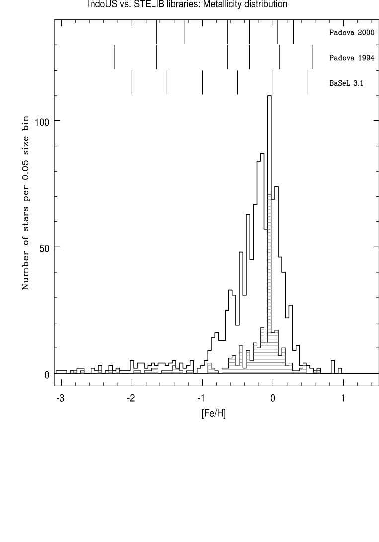
Figure 1.: Histogram showing the number of stars per 0.05 size bin in [Fe/H] for the IndoUS (dark line) and STELIB (hatched histogram) libraries. The values of [Fe/H] corresponding to the Padova 1994 and Padova 2000 sets of evolutionary tracks and the BaSeL 3.1 spectral atlas are shown as vertical lines at the top of the figure.

2. Stellar Libraries

A relatively large large number (5) of libraries containing medium to high spectral resolution observed spectra of excellent quality for large numbers of stars (hundreds to thousand) have become available during the recent past. One of the main objectives of the observers who invested large amounts of time and effort assembling these data sets was to build libraries suitable for population synthesis. In this respect, the stars in the libraries have been selected to provide broad coverage of the atmospheric parameters T_eff, log g, [Fe/H], as well as spectral type, throughout the HRD. In parallel to this observational effort, considerable progress has been made in the computation of theoretical model atmospheres at high spectral resolution for stars whose physical parameters are of interest for galaxy modeling. Below I describe very briefly the characteristics of each of these libraries which are relevant for population synthesis models.

2.1. HNGSL

The Hubble’s New Generation Spectral Library (Heap & Lanz 2003) contains spectra for a few hundred stars whose fundamental parameters, including chemical abundance, are well known from careful analysis of the visual spectrum. The spectra cover fully the wavelength range from 1700 Å to 10,200 Å. The advantage of this library over the ones listed below is the excellent coverage of the near-UV and the range from 9000 Å to 10,200 Å, which is generally noisy or absent in the other data sets.

2.2. MILES

The Medium resolution INT Library of Empirical Spectra (Sánchez-Blázquez et al. 2005), contains carefully calibrated and homogeneous quality spectra for 1003 stars in the wavelength range 3500 Å to 7500 Å with 2 Å spectral resolution and dispersion 0.9 Å pixel^-1. The stars included in this library were chosen aiming at sampling stellar atmospheric parameters as completely as possible.

2.3. UVES POP library

The UVES Paranal Observatory Project (Bagnulo et al. 2004), has produced a library of high resolution ($R=\lambda/\Delta\lambda\approx 80,000$) and high signal-to-noise ratio spectra for over 400 stars distributed throughout the HRD. For most of the spectra, the typical final SNR obtained in the V band is between 300 and 500. The UVES POP library is the richest available database of observed optical spectral lines.

2.4. IndoUS library

The IndoUS library (Valdes et al. 2004) contains complete spectra over the entire 3460 Å to 9464 Å wavelength region for 885 stars obtained with the 0.9m Coudé Feed telescope at KPNO. The spectral resolution is $\approx$ 1 Å and the dispersion 0.44 Å pixel^-1. The library includes data for an additional 388 stars, but only with partial spectral coverage.

2.5. ELODIE

The ELODIE library is a stellar database of 1959 spectra for 1503 stars, observed with the échelle spectrograph ELODIE on the 193 cm telescope at the Observatoire de Haute Provence. The resolution of this library is $R=42,000$ in the wavelength range from 4000 Å to 6800 Å (Prugniel & Soubiran 2001a, b). This library has been updated, extended, and used by Le Borgne et al. (2004) in the version 2 of the population synthesis code PEGASE.

2.6. High-spectral resolution theoretical libraries

There are several on-going efforts to improve the existing grids of theoretical model atmospheres including the computation of high resolution theoretical spectra for stars whose physical parameters are of interest for population synthesis. See, for example, Coelho et al. (2005); Bertone et al. (2004); Murphy & Meiksin (2004); Peterson et al. (2004), as well as the papers by Chávez, Bertone, Buzzoni & Rodríguez-Merino; González-Delgado & Cerviño; and Munari & Castelli in this conference.

3. Using the New Libraries in Population Synthesis Models

In BC03 the ’standard’ reference model represents a simple stellar population (SSP) computed using the Padova 1994 evolutionary tracks, the Chabrier (2003) IMF truncated at 0.1 and 100 M_⊙, and either the STELIB, the Pickles, or the BaSeL 3.1 spectral libraries (see BC03 for details). Below I show the behavior of the standard reference model computed with the IndoUS and the HNGSL libraries, and the Coelho et al. (2005) atlas of theoretical model atmospheres.

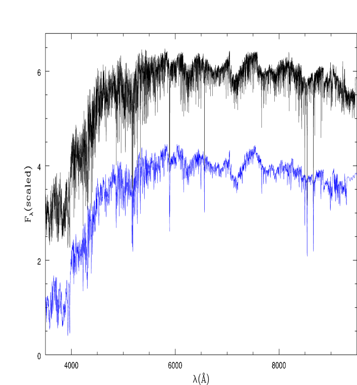
Figure 2.: BC03 standard SSP model spectra for solar metallicity at 12 Gyr in the wavelength range from 3500 Å to 9500 Å computed with the IndoUS (top line) and the STELIB (bottom line) libraries. The spectra have been scaled and shifted in the vertical direction for clarity.

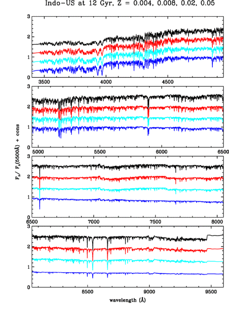
Figure 3.: BC03 standard SSP model spectra for Z = 0.004, 0.008, 0.02, and 0.05 (top to bottom) at 12 Gyr in the wavelength range from 3500 to 9500 Å built using the IndoUS stellar library. The spectra have been normalized and shifted arbitrarily in the vertical direction for clarity.

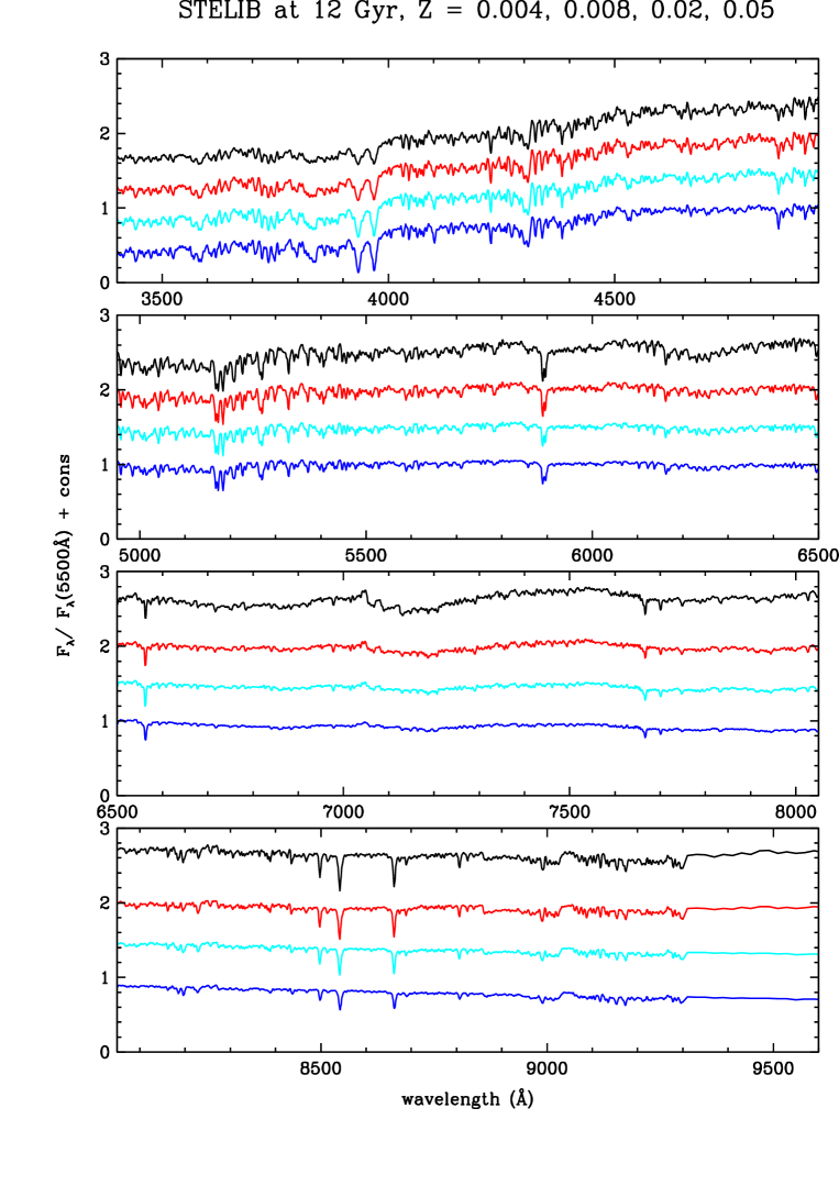
Figure 4.: BC03 standard SSP model spectra for Z = 0.004, 0.008, 0.02, and 0.05 (top to bottom) at 12 Gyr in the wavelength range from 3500 to 9500 Å built using the STELIB stellar library. The spectra have been normalized and shifted arbitrarily in the vertical direction for clarity.

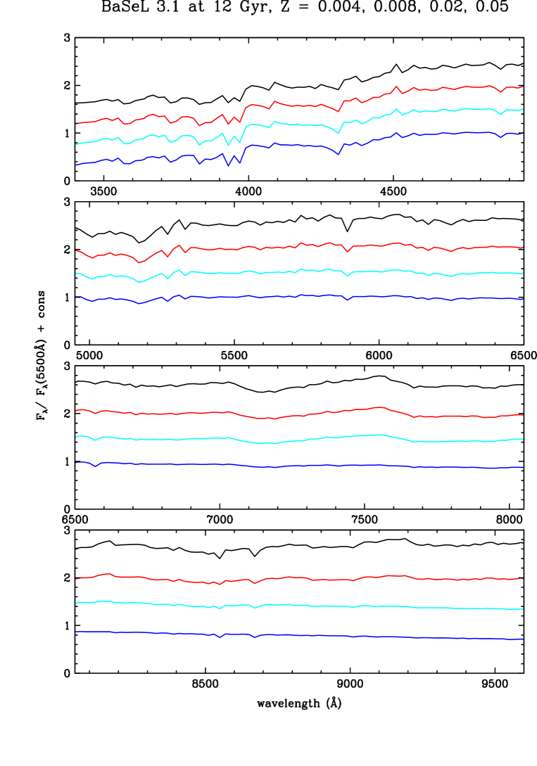
Figure 5.: BC03 standard SSP model spectra for Z = 0.004, 0.008, 0.02, and 0.05 (top to bottom) at 12 Gyr in the wavelength range from 3500 to 9500 Å built using the BaSeL 3.1 spectral atlas. The spectra have been normalized and shifted arbitrarily in the vertical direction for clarity.

3.1. IndoUS library

Figure 1 shows a histogram of the number of stars per 0.05 size bin in [Fe/H] for both the IndoUS and the STELIB libraries. The gain in the number of stars available at most metallicities in the IndoUS library with respect to STELIB shows clearly in this plot. This should translate in a better sampling of most stellar types at the relevant positions in the HRD for the metallicities corresponding to the different evolutionary tracks, also shown in Figure 1. Models built using the IndoUS library are compared to the STELIB and BaSeL 3.1 models in Figures 2 to 5. As expected, spectral features are more numerous and more clearly seen in the IndoUS model than in the other two models. Colors measured from the continuum flux in these three spectra are all very similar.

Figures 6 and 7 show the normalized residual distributions resulting from simultaneous fits of the strengths of several indices in the spectra of 2010 galaxies with S/N${}_{\rm med}\geq 30$ in the ‘main galaxy sample’ of the SDSS EDR using BC03 models built with the STELIB and the IndoUS libraries, respectively. The highlighted frames indicate the seven indices used to constrain the fits. The stellar velocity dispersion of the models are required to be within 15 km s^-1 of the observed ones. Each panel shows the distribution of the fitted index strength $I^{\rm fit}$ minus the observed one $I^{\rm obs}$, divided by the associated error $\sigma_{I}$. For reference, a dotted line in each panel indicates a Gaussian distribution with unit standard deviation. The shaded histograms show the contributions to the total distributions by galaxies with $\sigma_{V}>180$ km s^-1, corresponding roughly to the median stellar velocity dispersion of the sample. Figure 6 is identical to Figure 18 of BC03. It is apparent from a comparison of these two figures that the CN₁, CN₂, Ca4227, G4300, TiO₁, and TiO₂ indices measured in this galaxy sample are reproduced more closely by the IndoUS models than the STELIB models. The Mg₁, Mg₂, Mgb, and NaD indices are equally off in both sets of models. The negative residuals indicate that the model values are below the observed ones, due to the lack of stars with enhanced $\alpha$ element abundance in these stellar libraries. The distributions for H$\beta$ and H$\delta_{A}$ in the IndoUS models are shifted toward positive and negative residual values, respectively, with respect to the STELIB models. The four [MgFe] indices shown in the bottom row of Figures 6 and 7 are all shifted toward negative residuals in the IndoUS models.

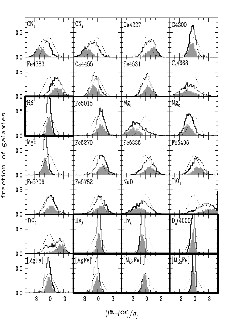
Figure 6.: Simultaneous fit of the strengths of several indices in the spectra of 2010 galaxies with S/N${}_{\rm med}\geq 30$ in the ‘main galaxy sample’ of the SDSS EDR using BC03 models built with the STELIB library. The highlighted frames indicate the seven indices used to constrain the fits. The stellar velocity dispersion of the models are required to be within 15 km s^-1 of the observed ones. Each panel shows the distribution of the fitted index strength $I^{\rm fit}$ minus the observed one $I^{\rm obs}$, divided by the associated error $\sigma_{I}$. For reference, a dotted line in each panel indicates a Gaussian distribution with unit standard deviation. The shaded histograms show the contributions to the total distributions by galaxies with $\sigma_{V}>180$ km s^-1, corresponding roughly to the median stellar velocity dispersion of the sample. This figure is identical to Figure 18 of BC03.

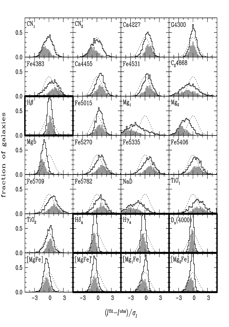
Figure 7.: Simultaneous fit of the strengths of several indices in the spectra of 2010 galaxies with S/N${}_{\rm med}\geq 30$ in the ‘main galaxy sample’ of the SDSS EDR using BC03 models built with the IndoUS library. The highlighted frames indicate the seven indices used to constrain the fits. The stellar velocity dispersion of the models are required to be within 15 km s^-1 of the observed ones. Each panel shows the distribution of the fitted index strength $I^{\rm fit}$ minus the observed one $I^{\rm obs}$, divided by the associated error $\sigma_{I}$. For reference, a dotted line in each panel indicates a Gaussian distribution with unit standard deviation. The shaded histograms show the contributions to the total distributions by galaxies with $\sigma_{V}>180$ km s^-1, corresponding roughly to the median stellar velocity dispersion of the sample.

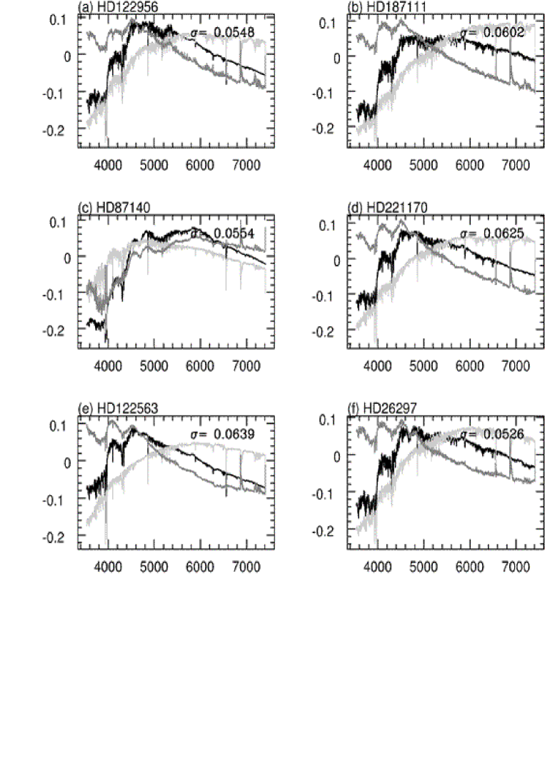
Figure 8.: Comparison of the sed’s of 6 stars present in the IndoUS and the MILES stellar libraries in the wavelength range $\lambda\lambda$ 3500 - 7400 Å in common in these libraries. In each panel the black line is the IndoUS sed, the light gray line is the MILES sed, and the dark gray line represents the difference (IndoUS - MILES). The sed’s have been scaled arbitrarily in the flux scale. The star identification is indicated in the upper left corner of each panel.

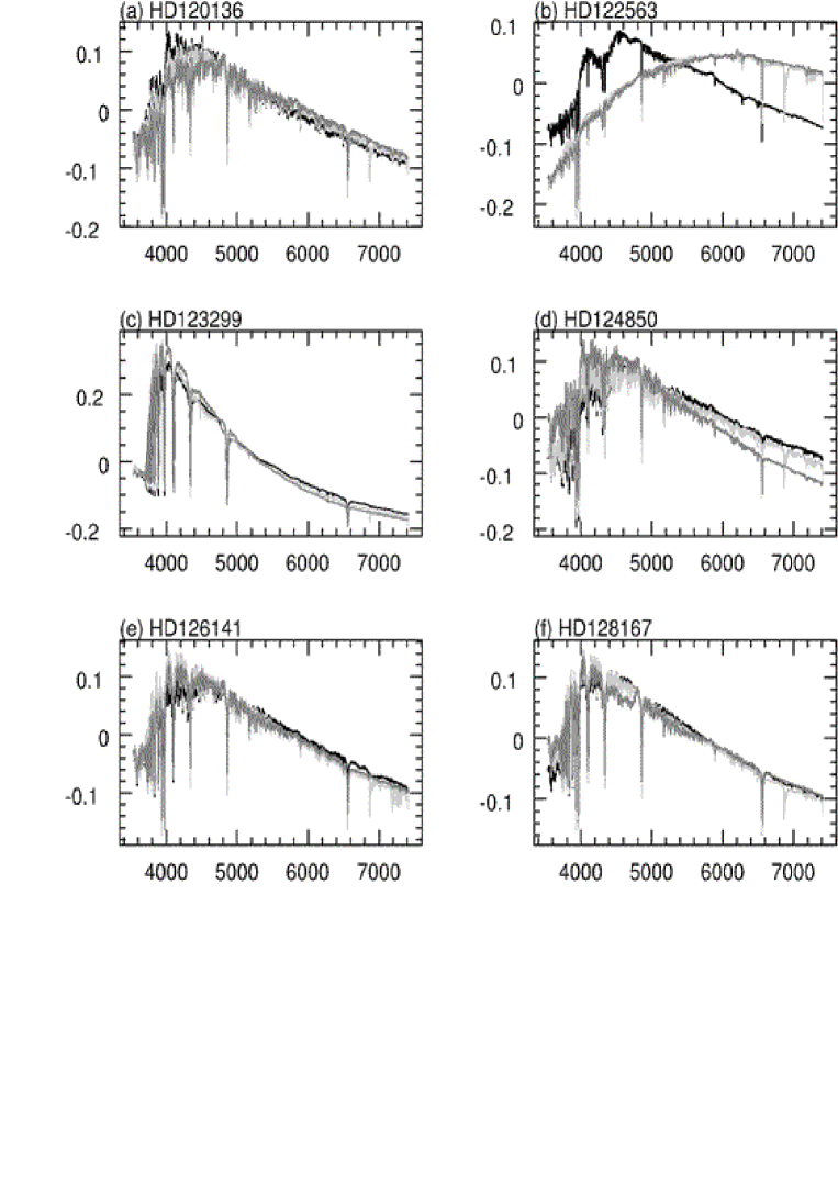
Figure 9.: Comparison of the sed’s of 6 stars present in the IndoUS, the STELIB, and the MILES stellar libraries in the wavelength range $\lambda\lambda$ 3500 - 7400 Å in common in these libraries. In each panel the black line is the IndoUS sed, the light gray line is the MILES sed, and the dark gray the STELIB sed. The sed’s have been scaled arbitrarily in the flux scale. The star identification is indicated in the upper left corner of each panel.

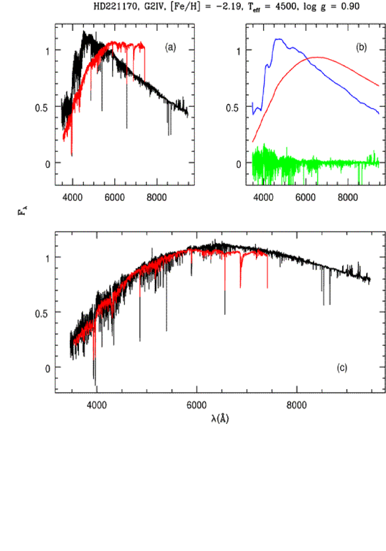
Figure 10.: Spectral energy distributions of the star HD221170. (a). The MILES sed extends up to 7400 Å and the IndoUS sed up to 9500 Å. (b). Smoothed version of the IndoUS sed for this star and of the BaSeL 3.1 model for $T_{eff}$ = 4500K, log g = 1, and [Fe/H] = -2, corresponding to the tabulated values for HD221170. The residual line in the bottom part of the panel is the difference between the original and the smoothed IndoUS sed’s. (c). Result of adding the smoothed BaSeL sed to the difference of the original and smoothed IndoUS sed’s shown in frame (b).

Flux calibration problems in the IndoUS library.

In Figure 8 I compare the spectra of 6 of the more than 500 stars in common between the IndoUS and the MILES libraries. These plots illustrate a flux calibration problem affecting some of the IndoUS spectra. Figure 9 shows spectra of 6 of the stars in common in the IndoUS, the MILES, and the STELIB libraries. For all the stars in common in the three libraries, the shape of the MILES and STELIB spectra always match, whereas if there is a discrepancy it can always be attributed to the IndoUS spectrum, as in the case of the star HD122563 in the upper right hand side panel of Figure 9. The IndoUS spectra of stars with flux calibration problems should not be used in population synthesis unless they can be re-calibrated correctly. In Figure 10 I indicate a procedure that uses the BaSeL 3.1 spectrum for the values of $T_{eff}$, log g, and [Fe/H] of the problem star to define the correct shape of the IndoUS spectrum. This procedure assumes that the physical parameters of the star are known accurately.

3.2. HNGSL

I have also computed the BC03 standard model using the HNGSL (Heap & Lanz 2003) instead of STELIB to represent the stellar spectra. Figure 11 shows clearly the advantages of using the HNGSL to study the near UV below 3300 Å. Spectral features, lines and discontinuities, are much better defined in the HNGSL spectra than in the IUE spectra (used in the Pickles library) and the BaSeL 3.1 atlas (see BC03 and Bruzual (2004) for details). However, colors measured from the continuum flux in these three spectra are very similar. The higher spectral resolution of STELIB above 3300 Å compared to HNGSL is clearly seen in this figure.

The spectra in Figure 12 are useful to study the different behavior of models computed with different libraries in the region around and above 9000 Å. There is a clear difference in the continuum level predicted by the HNGSL and STELIB models (lowest level) compared to the level predicted by the BaSeL 3.1 and the Pickles library models (highest level). The HNGSL model is to be preferred, given the higher SNR of this spectrum in this region. However, spectral features below 8500 Å are more clearly seen in the higher resolution STELIB model.

3.3. Theoretical model atmospheres

Figures 13 and 14 show the BC03 standard SSP model sed at 12 Gyr computed with the high resolution theoretical model atmospheres from the IAG collaboration for [Fe/H] = 0, $[\alpha/Fe]=0$, in the wavelength range from 0.3 to 18 $\mu$m (Coelho et al. 2005). In Figure 14 one can clearly see those regions of the spectrum where the theoretical atmosphere models produce different results from the empirical library models, e.g., above 9000 Å. In Figure 15 I compare the STELIB and IndoUS models with the IAG collaboration model degraded in spectral resolution to match the empirical spectra. This figure shows a remarkable degree of agreement between the empirical and theoretical models when the difference in resolution is duly taken into account. This figure replaces the one I showed in my oral presentation which contained an involuntary error in the procedure used to downgrade the spectral resolution of the theoretical model.

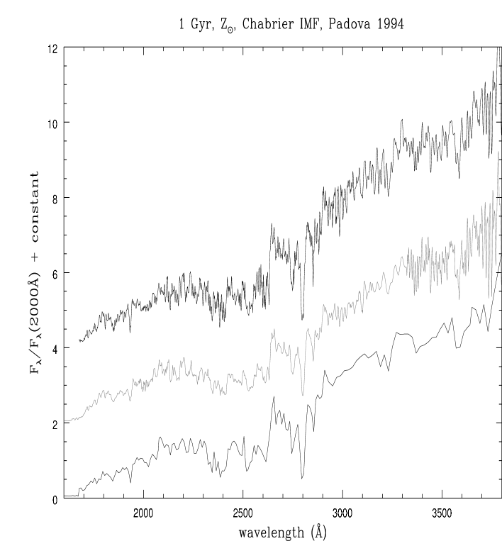
Figure 11.: BC03 standard SSP model spectra for solar metallicity at 1 Gyr in the wavelength range from 1600 Å to 3800 Å. The spectrum on top (thick black line) is built using the HNGSL, the one in the middle (gray line) uses the Pickles library and STELIB, and the bottom one (thin black line) the BaSel 3.1 library. The spectra have been normalized at 2000 Å and shifted arbitrarily in the vertical direction for clarity.

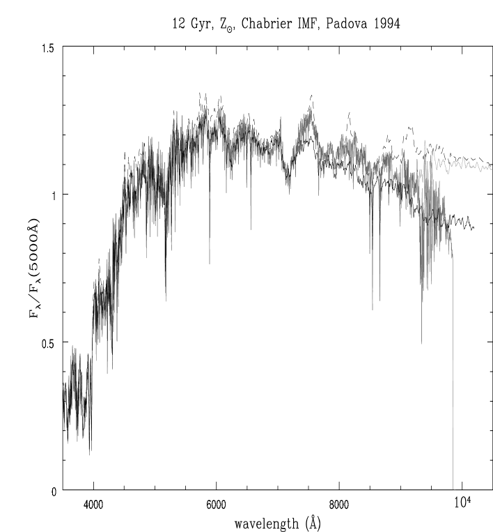
Figure 12.: BC03 standard SSP model spectra for solar metallicity at 12 Gyr in the wavelength range from 3500 Å to 10,500 Å. The black solid line (reaching up to 10,200 Å) represents the spectrum built using the HNGSL, the dark gray solid line (noisy above 9000 Å) uses STELIB, the light gray solid line uses STELIB up to 9000 Å and the Pickles library at longer wavelengths, the black dashed line uses the BaSel 3.1 library. The spectra have been normalized at 5000 Å.

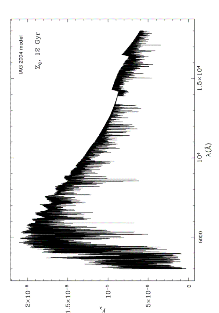
Figure 13.: BC03 standard SSP model sed at 12 Gyr computed with the high resolution theoretical model atmospheres from the IAG collaboration for [Fe/H] = 0, $[\alpha/Fe]=0$ (Coelho et al. 2005) in the wavelength range from 0.3 to 18 $\mu$m.

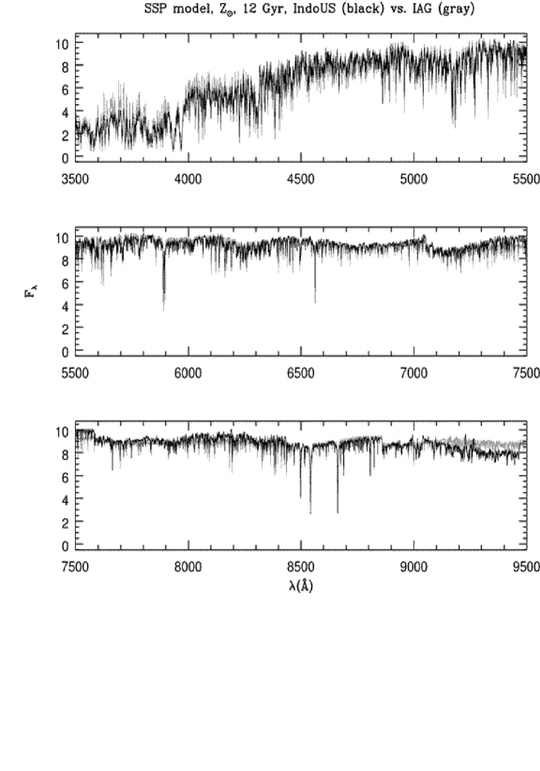
Figure 14.: BC03 standard SSP model sed at 12 Gyr computed with the high resolution theoretical model atmospheres from the IAG collaboration for [Fe/H] = 0, $[\alpha/Fe]=0$ (Coelho et al. 2005) in the wavelength range from 3500 to 9500 Å (gray line) downgraded to the spectral resolution of the IndoUS library. For comparison, the corresponding model computed with the IndoUS stellar library is shown as a black line.

Figure 15.: BC03 standard SSP model sed at 12 Gyr computed with the high resolution theoretical model atmospheres from the IAG collaboration for [Fe/H] = 0, $[\alpha/Fe]=0.0$ (Coelho et al. 2005), in the wavelength range from 5000 to 5200 Å containing the Mg₁, Mg₂, and Mgb features. The thin lines show the IAG model downgraded to the spectral resolution of the STELIB and IndoUS libraries, shown as heavy lines. The spectra have been scaled and shifted arbitrarily in the vertical direction.

4. Reproducing Galaxy SEDs

4.1. SSP fits

By means of a standard least-squares technique it is possible to select the age and stellar velocity dispersion at which a given SSP model reproduces most closely a given observed galaxy spectrum. Figures 16 to 18 show remarkably good fits to the continuum spectrum of three galaxies with different ages and velocity dispersions, and in different wavelength intervals. The BC03 standard SSP model computed with the IndoUS stellar library was used in these fits. The stellar velocity dispersion $\sigma$ indicated in each figure and applied to the model spectrum is also derived by the fitting algorithm. The residuals (observed - model) shown at the bottom of the plots are quite flat over the whole spectral range.

4.2. Non-parametric CSP fits

An alternative approach for studying the stellar populations present in a galaxy, based on the fact that galaxies are thought to be more closely described by a composite stellar population (CSP) rather than by an SSP, consists in deriving the galaxy star formation history (SFH) by means of a non-parametric CSP fit to the galaxy sed. In a non-parametric fit the SFH is not assumed to be described by an analytic function, e.g., an exponentially decaying star formation rate with characteristic $e-$folding time $\tau$. Instead, all the spectra defining the evolution of an SSP of one or more metallicity values are allowed to be selected individually by a spectral fitting algorithm. The SFH for the galaxy is rebuilt from the known age and metallicity of each of the selected spectra. See Mateu, Magris, & Bruzual (2005) for a description of GASPEX, a non-parametric CSP fitting procedure based on the Non-Negative Least Squares (NNLS) algorithm of Lawson and Hanson (1974).

The SFH recovered by this type of algorithm is highly dependent on the signal-to-noise ratio and the wavelength range covered by the problem spectrum. Figures 19 and 20 show the results of applying the GASPEX algorithm to a problem spectrum of known SFH. The problem spectrum corresponds to an old stellar population of age 6 Gyr in which a second burst of star formation of $1\over 9$ the intensity of the first burst occurs 360 Myr ago. In these figures, the two vertical lines at the corresponding ages represent schematically this SFH. The histograms with error bars in Figure 19 represent the SFH recovered by the GASPEX algorithm when noise in varying amounts is added to the problem spectrum. The value of the signal-to-noise ratio (SNR) used is indicated in each frame. Values of SNR above 10 are required to recover the input SFH. Similarly, Figure 20 shows that the broader the wavelength range covered by the problem spectrum, the more likely it is that we recover the input SFH. For the example in Figure 20, the problem spectrum is the same one used in Figure 19 for a signal-to-noise ratio of 20. The full coverage of the wavelength range from the UV to the IR is required to recover the known SFH.

Figure 21 shows the SFH and cumulative mass vs. age function recovered by the GASPEX algorithm for a selection of galaxies from the Near Field Galaxy Survey (Jansen et al. 2000). The thin lines represent galaxies with significant recent star formation, as indicated by the emission lines in their spectra. It is apparent from this plot that these galaxies assemble their stars at a later time than the early-type galaxies represented by the heavy lines in Figure 21.

4.3. SSP vs. CSP fitting

Figure 22 shows the best SSP model fit to the spectrum of an early type galaxy resulting from co-adding the spectra of several galaxies from the SDSS until reaching a signal-to-noise ratio of 250. This spectrum, kindly provided by Jarle Brinchmann, is shown as a gray line in the wavelength range from 3600 to 7500 Å. The BC03 standard SSP model computed with the STELIB stellar library for solar metallicity at an age of 9.25 Gyr is shown in black. The stellar velocity dispersion $\sigma=280$ km s^-1 applied to the model spectrum is also derived by the fitting algorithm. At the bottom of the figure the line marked SSP represents the residuals (observed -model) for the SSP model fit shown in the figure. The line marked CSP represents the residuals obtained when the fit is performed by the non-parametric GASPEX CSP fitting algorithm described by Mateu, Magris, & Bruzual (2005). The line marked S-C shows the difference between the SSP and CSP solutions (shifted down arbitrarily for clarity).

The top frame of Figure 23 shows the cumulative squared residuals ($\propto\chi^{2}$) for the SSP and CSP fits shown in Figure 22. The CSP fit reaches a lower $\chi^{2}$ value. The improved fit over the SSP fit is achieved by the GASPEX algorithm by assuming that some star formation happened in this galaxy at ages younger than the SSP age of 9 Gyr. The vertical lines show the position of the central bands defining the CN₁-CN₂, Mg₁-Mg₂-Mgb, and NaD Lick indices, and the H$\alpha$ line. The lower residuals in the CSP fit are possible because the younger population fills in the deficiency of the SSP model at the bands containing the Mg and Na features, i.e. the steep increase in $\chi^{2}$ seen at these wavelengths in the SSP fit are not present in the CSP fit. On the other hand, the CN features are reproduced best by the SSP model. The H$\alpha$ emission line is not included in neither of the models. The same is true for the apparent features in the observed spectrum at $\lambda>6700$ Å. Beyond H$\alpha$ the two $\chi^{2}$ functions run almost parallel.

The middle frame of figure 23 shows the percentage contribution of the old and a very young population (100 Myr) to the total spectrum of this galaxy in the CSP solution as a function of wavelength. The contribution of populations of other ages included in the GASPEX solution is, added all together, below the 5% level at $\lambda<4500$ Å, and is even less at longer wavelengths. The spectra corresponding to the old, young, and the rest of the stellar populations in the GASPEX solution are shown in the bottom frame of this figure. The latter contribute essentially zero flux to the total sed. The heavy line in this frame represents the CSP solution, i.e., the addition of the individual spectra.

The fact that the best GASPEX solution has a lower $\chi^{2}$ and requires recent star formation does not necessarily imply that it represents a more realistic solution than the SSP fit from the astrophysical point of view. However, the GASPEX non-parametric CSP solution for this galaxy es reminiscent of the E+A phenomenon, quite common in E galaxies. The fact that the CSP solution seems able to detect the E+A phenomenon makes this technique appealing.

Figure 24 shows a detailed comparison of the fit to one of J. Brinchmann co-added spectra in specific wavelength regions. The residuals in the second, fourth and sixth panels are expressed in units of the standard deviation $\sigma$ of the co-added fluxes. The signal-to-noise ratio in these spectra is so high, and $\sigma$ so low, that the very small differences between the problem and solution spectra translate into very large residuals when measured in units of $\sigma$. Thus, very careful analysis of the fits should be performed when deriving galaxy SFHs.

5. Conclusions

New libraries of empirical spectra of stars covering wide ranges of values of the atmospheric parameters T_eff, log g, [Fe/H], as well as spectral type, that have become available recently, are complementary in spectral resolution and wavelength coverage.

Models built using the IndoUS and the HNGSL empirical stellar libraries, and the IAG collaboration theoretical model atmospheres, show that this sort of library will prove extremely useful in describing spectral features expected in galaxy spectra of various ages and metallicities from the NUV to the NIR.

Models build with the IndoUS library increase the number of Lick indices that are correctly reproduced by the models.

The use of population synthesis models to derive galaxy star formation histories by fitting galaxy spectra have become very popular in recent years. The reader should keep in mind that different solutions are provided by the simple minimum $\chi^{2}$ SSP fit and the more complex non-parametric CSP fit. Even if the CSP fits result in a lower value of $\chi^{2}$, the solutions are not necessarily more sound from astrophysical grounds. The fact that the CSP solution seems able to detect the E+A phenomenon makes this technique appealing.

Complete sets of models that use the libraries mentioned in §2 are been built and will be discussed in a coming paper by Bruzual & Charlot.

Acknowledgments.

I thank Jarle Brinchmann for providing me with his sample of co-added SDSS spectra.

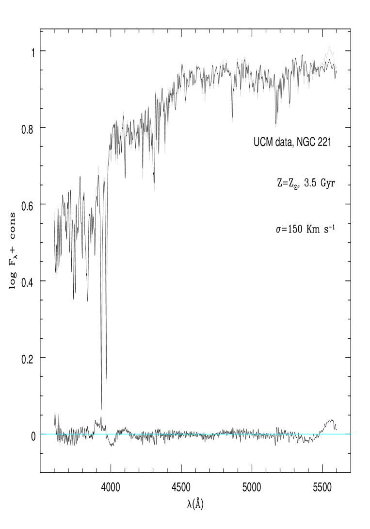
Figure 16.: Best SSP model fit to the spectrum of the elliptical galaxy NGC 221 in the wavelength range from 3600 to 5600 Å. The BC03 standard SSP model computed with the IndoUS stellar library for solar metallicity at an age of 3.5 Gyr is shown in black. The stellar velocity dispersion $\sigma=150$ km s^-1 applied to the model spectrum is also derived by the fitting algorithm. The observed spectrum is shown in gray and was kindly provided by P. Sánchez-Blázquez. The residuals (observed - model) are shown at the bottom of the plot in the same vertical scale.

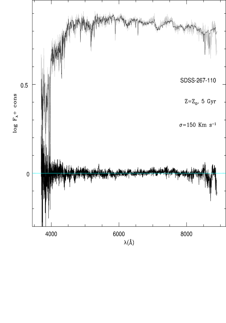
Figure 17.: Best SSP model fit to the spectrum of the early-type galaxy SDSS-267-110 in the wavelength range from 3750 to 8800 Å. The BC03 standard SSP model computed with the IndoUS stellar library for solar metallicity at an age of 5 Gyr is shown in black. The stellar velocity dispersion $\sigma=150$ km s^-1 applied to the model spectrum is also derived by the fitting algorithm. The SDSS-EDR observed spectrum is shown in gray. The residuals (observed - model) are shown at the bottom of the plot in the same vertical scale.

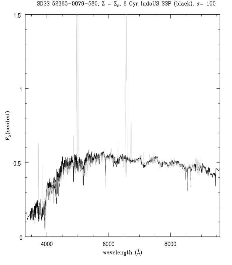
Figure 18.: Best SSP model fit to the continuum spectrum of the star forming galaxy SDSS-52365-0879-580 in the wavelength range from 3500 to 9500 Å. The BC03 standard SSP model computed with the IndoUS stellar library for solar metallicity at an age of 6 Gyr is shown in black. The stellar velocity dispersion $\sigma=100$ km s^-1 applied to the model spectrum is also derived by the fitting algorithm. The SDSS-EDR observed spectrum is shown in gray. The wavelength ranges containing emission lines in the observed spectrum are not included in the fit.

Figure 19.: Recovery of a known star formation history as a function of the signal-to-noise ratio of the problem spectrum. The problem spectrum corresponds to an old stellar population of age 6 Gyr in which a second burst of star formation of $1\over 9$ the intensity of the first burst occurs 360 Myr ago. The two vertical lines at the corresponding ages represent schematically this star formation history. The histograms with error bars represent the star formation history recovered by the GASPEX non-parametric CSP fitting algorithm described by Mateu, Magris, & Bruzual (2005) when noise is added to the problem spectrum. The value of the signal-to-noise ratio (SNR) used is indicated in each frame.

Figure 20.: Recovery of a known star formation history as a function of wavelength coverage. The problem spectrum is the same one used in Figure 19 for a signal-to-noise ratio of 20. The histograms with error bars represent the star formation history recovered by the GASPEX non-parametric CSP fitting algorithm described by Mateu, Magris, & Bruzual (2005) as a function of the wavelength range used in the fit, as indicated in each frame.

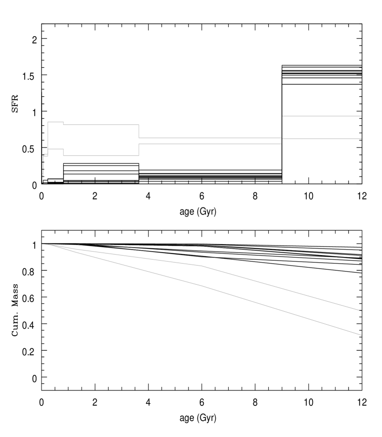
Figure 21.: Star formation history and cumulative mass vs. age recovered by the GASPEX non-parametric CSP fitting algorithm described by Mateu, Magris, & Bruzual (2005) for a selection of galaxies from the Near Field Galaxy Survey (Jansen et al. 2000). The gray lines represent galaxies with significant recent star formation, as indicated by the emission lines in their spectra.

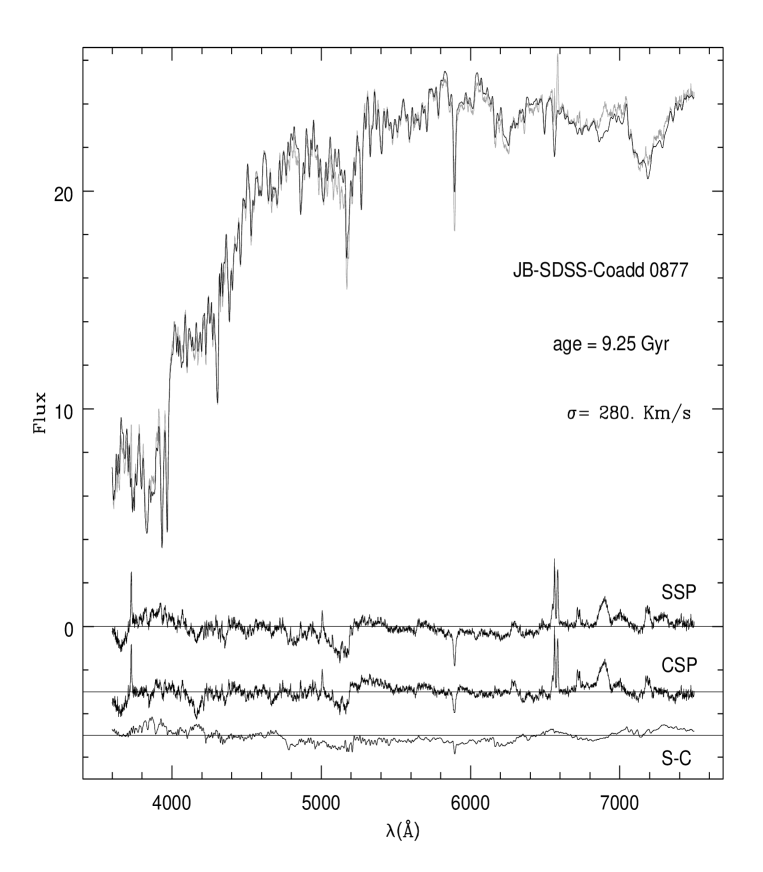
Figure 22.: Best model fit to the spectrum of an early type galaxy resulting from co-adding the spectra of several galaxies from the SDSS until reaching a signal-to-noise ratio of 250. This spectrum, kindly provided by Jarle Brinchmann, is shown as a light line in the wavelength range from 3600 to 7500 Å. The BC03 standard SSP model computed with the STELIB stellar library for solar metallicity at an age of 9.25 Gyr is shown as a heavy line. The stellar velocity dispersion $\sigma=280$ km s^-1 applied to the model spectrum is also derived by the fitting algorithm. At the bottom of the figure the line marked SSP represents the residuals (observed -model) for the SSP model shown in the figure. The line marked CSP represents the residuals obtained when the fit is performed by the GASPEX non-parametric CSP fitting algorithm described by Mateu, Magris, & Bruzual (2005). The line marked S-C shows the difference between the SSP and CSP solutions. The last two lines have been shifted down for clarity.

Figure 23.: Top frame. Cumulative squared residuals for the SSP and CSP fits shown in Figure 22. The vertical lines show the position of the central bands defining the CN₁-CN₂, Mg₁-Mg₂-Mgb, and NaD Lick indices, and the H$\alpha$ line. Middle frame. Percentage contribution of the old and a very young population (100 Myr) to the total spectrum of this galaxy in the CSP solution as a function of wavelength. The contribution of populations of other ages included in the GASPEX solution is, added all together, below the 5% level at $\lambda<4500$ Å, and is even less at longer wavelengths. Bottom frame. Spectra corresponding to the old, young, and the rest of the stellar populations in the GASPEX solution. The latter contribute essentially zero flux to the total sed, represented by the heavy line.

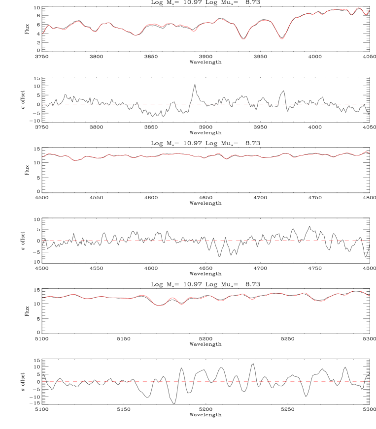
Figure 24.: Detailed comparison of the fit to one of J. Brinchmann co-added spectrum in specific wavelength regions. The residuals in the second, fourth and sixth panels are expressed in units of the standard deviation $\sigma$ of the co-added fluxes.

References

- Bagnulo et al. (2004) Bagnulo, S., Jehin, E., Ledoux, C., Cabanac, R., Melo, C., Gilmozzi, R. and the ESO Paranal Science Operations Team 2003, The Messenger, 114, 10
- Bertone et al. (2004) Bertone, E., Buzzoni, A., Rodríguez-Merino, L. H., & Chávez, M. 2004, MmSAI, 75, 158
- Bruzual (2004) Bruzual A., G. 2004, in Proceedings of the IAU Symposium No. 222 “The Interplay Among Black Holes, Stars, and ISM in Galactic Nuclei”, eds. T. Storchi-Bergmann, L.C. Ho, and H.R. Schmitt, Cambridge: Cambridge University Press, 121
- Bruzual & Charlot (2003) Bruzual A., G. & Charlot, S. 2003, MNRAS, 344, 1000
- Chabrier (2003) Chabrier, G. 2003, PASP, 115, 763
- Cid-Fernandes et al. (2005) Cid-Fernandes, R., Mateus, A., Laerte, S. Jr, Stasinska, G., & Gomes, J. M. 2005, MNRAS, 358, 363
- Coelho et al. (2005) Coelho, P., Barbuy, B., Melendez, J., Schiavon, R., & Castilho, B. 2005. A&A (in press), astro-ph/0505511
- Heap & Lanz (2003) Heap, S. R., & Lanz, T. 2003, in Proceedings of the ESO-USM-MPE “Workshop on Multiwavelength Mapping of Galaxy Formation and Evolution”, ESO Astrophysics Symposia, eds. R. Bender and A. Renzini
- Heavens et al. (2004) Heavens, A., Panter, B., Jiménez, R., & Dunlop, J. 2004, Nature, 428, 625
- Jansen et al. (2000) Jansen, R., Franx, M., Fabricant, D.,Caldwell, N. 2000, ApJS, 126, 331
- Lawson and Hanson (1974) Lawson, C. L., & Hanson, R. J. 1974, Solving Least Squares Problems, Prentice Hall Inc., Englewood Cliffs, New Jersey
- Le Borgne et al. (2003) Le Borgne, J.-F., Bruzual A., G., Pelló, R., Lançon, A., Rocca-Volmerange, B., Sanahuja, B., Schaerer, D., Soubiran, C., & Vílchez-Gómez, R. 2003, A&A, 402, 433
- Le Borgne et al. (2004) Le Borgne, D., Rocca-Volmerange, B., Prugniel, P., Lançon, A., Fioc, M., & Soubiran, C. 2004, A&A, 425, 881
- Lejeune, Cuisinier, & Buser (1997) Lejeune, T., Cuisinier, F., & Buser, R. 1997, A&AS, 125, 229
- Lejeune, Cuisinier, & Buser (1998) Lejeune, T., Cuisinier, F., & Buser, R. 1998, A&AS, 130, 65
- Mateu, Magris, & Bruzual (2005) Mateu, J., Magris C., G. & Bruzual A., G. 2005, MNRAS (in preparation)
- Murphy & Meiksin (2004) Murphy, T., & Meiksin, A. 2004, astro-ph/0404010
- Peterson et al. (2004) Peterson, R. C., Carney, B. W., Dorman, B., Green, E. M., Landsman, W., Liebert, J., O’Connell, R. W., Rood, R. T., & Schiavon, R. P. 2004, AAS, 204, 07.08
- Pickles (1998) Pickles, A. J. 1998, PASP, 110, 863
- Prugniel & Soubiran (2001a) Prugniel, P., & Soubiran, C. 2001a, A&A, 369, 1048
- Prugniel & Soubiran (2001b) Prugniel, P., & Soubiran, C. 2001b, VizieR Online Data Catalog, 3218
- Sánchez-Blázquez et al. (2005) Sánchez-Blázquez, P., Peletier, R.F., Jiménez-Vicente, J., Cardiel, N., Falcón-Barroso, J., Gorgas, J., Selam, S. & Vazdekis, A. 2005, MNRAS (submitted)
- Seaton (1979) Seaton M. J. 1979, MNRAS, 187, 73
- Stoughton et al. (2002) Stoughton et al. 2002, AJ, 123, 485
- Valdes et al. (2004) Valdes, F., Gupta, R., Rose, J. A., Singh, H. P., & Bell, D. J. 2004, ApJS, 152, 251
- Westera et al. (2002) Westera, P., Lejeune, T., Buser, R., Cuisinier, F., & Bruzual A., G. 2002, A&A, 381, 524