An XMM-Newton Observation of the Local Bubble using a Shadowing Filament in the Southern Galactic Hemisphere

Abstract

We present an analysis of the X-ray spectrum of the Local Bubble, obtained by simultaneously analyzing spectra from two XMM-Newton pointings on and off an absorbing filament in the Southern galactic hemisphere ($b\approx-45\arcdeg$). We use the difference in the Galactic column density in these two directions to deduce the contributions of the unabsorbed foreground emission due to the Local Bubble, and the absorbed emission from the Galactic halo and the extragalactic background. We find the Local Bubble emission is consistent with emission from a plasma in collisional ionization equilibrium with a temperature $\log(T_{\mathrm{LB}}/\mathrm{K})=6.06^{+0.02}_{-0.04}$ and an emission measure $\int n_{\mathrm{e}}^{2}\mathrm{d}l=0.018$ $\mbox{cm}^{-6}$ pc. Our measured temperature is in good agreement with values obtained from ROSAT All-Sky Survey data, but is lower than that measured by other recent XMM-Newton observations of the Local Bubble, which find $\log(T_{\mathrm{LB}}/\mathrm{K})\approx 6.2$ (although for some of these observations it is possible that the foreground emission is contaminated by non-Local Bubble emission from Loop I). The higher temperature observed towards other directions is inconsistent with our data, when combined with a FUSE measurement of the Galactic halo O vi intensity. This therefore suggests that the Local Bubble is thermally anisotropic.

Our data are unable to rule out a non-equilibrium model in which the plasma is underionized. However, an overionized recombining plasma model, while observationally acceptable for certain densities and temperatures, generally gives an implausibly young age for the Local Bubble ($\lesssim 6\times 10^{5}$ yr).

1. INTRODUCTION

The Local Bubble (LB) is a region of X-ray–emitting gas of $\sim$100 pc extent in which the Solar System resides. Measurements of the interstellar Na i absorption towards 456 nearby stars reveal that the Local Bubble resides in a cavity in the interstellar medium (ISM; Sfeir et al., 1999). The idea of the Local Bubble originated in the late 1970s, in order to explain the observed anticorrelation between the intensity of the soft X-ray background (SXRB) and the Galactic hydrogen column density $N_{\mathrm{H}}$ (Bowyer et al., 1968; Sanders et al., 1977). The data are inconsistent with the anticorrelation being due to absorption, as they require an interstellar absorption cross-section that is one-third of its expected value (Bowyer et al., 1968), and also different energy bands have the same dependence on $N_{\mathrm{H}}$ (Sanders et al., 1977; Juda et al., 1991). Instead, a so-called “displacement” model was proposed, in which the hot X-ray–emitting plasma (the Local Bubble) is in the foreground and displaces the cool gas (Sanders et al., 1977; Tanaka & Bleeker, 1977). In directions of higher X-ray intensity the Local Bubble is thought to be of greater extent, and so there is less cool gas (and hence lower $N_{\mathrm{H}}$) in those directions.

Numerous models have been proposed for the formation of the Local Bubble (for reviews, see Breitschwerdt 1998; Cox 1998; Breitschwerdt & Cox 2004). These models may essentially be divided into two classes. In one class of model, the Local Bubble was carved out of the ambient ISM by a supernova or series of supernovae (e.g. Cox & Anderson, 1982; Innes & Hartquist, 1984; Smith & Cox, 2001; Maíz-Apellániz, 2001; Breitschwerdt & de Avillez, 2006). The hot gas thus produced gives rise to the observed X-rays. If the last supernova was recent enough, one would expect the ions to be underionized. However, if the Local Bubble is old enough to have begun contracting, the ions will be overionized and recombining (Smith & Cox, 2001). In the second class of model, a series of supernovae in a dense cloud formed a hot bubble, which burst out of the cloud into the less dense surroundings and underwent rapid adiabatic cooling (Breitschwerdt & Schmutzler, 1994; Breitschwerdt, 1996; Breitschwerdt et al., 1996; Breitschwerdt, 2001). In this case the X-ray emission is due to the delayed recombination of the overionized ions. X-ray spectroscopy of the Local Bubble emission is essential for distinguishing between the various models, as it enables us to determine the physical properties of the X-ray–emitting gas.

Originally, all the soft X-ray flux was attributed to the Local Bubble, which made determining the Local Bubble X-ray spectrum relatively simple. However, the discovery of shadows in the SXRB with ROSAT (Snowden et al., 1991; Burrows & Mendenhall, 1991) showed that $\sim$50% of the SXRB in the 1/4-keV band originated from beyond the Local Bubble, either in the Galactic halo or from an extragalactic background. Hence, in order to determine the Local Bubble spectrum, one must first disentangle the contributions of the Local Bubble and the background. This has been done by modeling ROSAT All-sky Survey data (RASS; Snowden et al., 1997) with an unabsorbed foreground component (due to the Local Bubble) and absorbed components for the Galactic halo and the extragalactic background, using the 100-µm Infrared Astronomical Satellite (IRAS) maps of Schlegel et al. (1998) as a measure of $N_{\mathrm{H}}$. In this way the Local Bubble emission has been mapped out, and its temperature estimated to be $T_{\mathrm{LB}}\sim 10^{6}$ K assuming collisional ionization equilibrium (Snowden et al., 1998, 2000; Kuntz & Snowden, 2000).

It should be noted, however, that the RASS data are presented in just six energy bands between $\sim$0.1 and $\sim$2 keV, several of which overlap. The data therefore have fairly poor spectral resolution. The Local Bubble temperature is inferred from the R1-to-R2 band intensity ratio of the local emission component, as there is very little Local Bubble emission in the higher-energy bands: the upper limit on the ROSAT R45 intensity due to the Local Bubble is a $\mbox{few}\times 10^{5}$ counts $\mbox{s}^{-1}$ arcmin^-2 (Snowden et al., 1993; Kuntz et al., 1997). However, this observational fact may be used to rule out significantly higher temperatures. It should also be noted that this inferred temperature is somewhat dependent upon the plasma emission model used (e.g. Kuntz & Snowden, 2000).

The large mirror collecting area and CCD detectors onboard XMM-Newton enable us to obtain high signal-to-noise spectra of the SXRB with greater spectral resolution than ROSAT. In particular, XMM-Newton enables us to detect line emission in the SXRB spectrum, notably emission from O vii and O viii at $\sim$0.55 and $\sim$0.65 keV. If we can determine how much of this oxygen emission is due to the Local Bubble, this will enable us to place stronger constraints on $T_{\mathrm{LB}}$.

We use a shadowing technique to determine the spectrum of the Local Bubble emission. We have analyzed spectra obtained from XMM-Newton pointings on and off an absorbing filament in the southern Galactic hemisphere. The absorbing filament appears as a shadow in the SXRB, as shown in Figure 1, which also shows our XMM-Newton pointing directions. Penprase et al. (1998) have estimated the distance of the filament to be $230\pm 30$ pc. Maps of the extent of the Local Bubble, obtained from RASS data (Snowden et al., 1998) and Na i absorption data (Sfeir et al., 1999; Lallement et al., 2003), indicate that the boundary of the Local Bubble is $\sim$100 pc away in this direction. Thus, the filament is between the Local Bubble and the Galactic halo. We fit spectral models simultaneously to the on- and off-filament spectra, using the difference in the absorbing column between the two pointing directions ($N_{\mathrm{H}}=9.6\times 10^{20}$ $\mbox{cm}^{-2}$ versus $1.9\times 10^{20}$ $\mbox{cm}^{-2}$; see §3.1) to deduce the contributions of the foreground (unabsorbed) and background (absorbed) model components to the observed spectra.

Our observations and the data reduction are described in §2. The spectral models used to fit to the data are described in §3, and the fit results are presented in §4. We discuss our results in §5. In particular, we compare our results with the results of RASS analyses in §5.1, and we compare our results’ prediction of the Galactic halo O vi intensity with the observed value in §5.2. In §5.3 we compare our results with those of other XMM-Newton and Chandra observations of the Local Bubble. In §5.4 we discuss our choice of plasma emission code used in the analysis, and consider the effect this has on our results. Finally in this section we discuss non-equilibrium models of the Local Bubble: an underionized model in §5.5, and a recombining model in §5.6. We conclude with a summary in §6. Throughout this paper we quote $1\sigma$ errors.

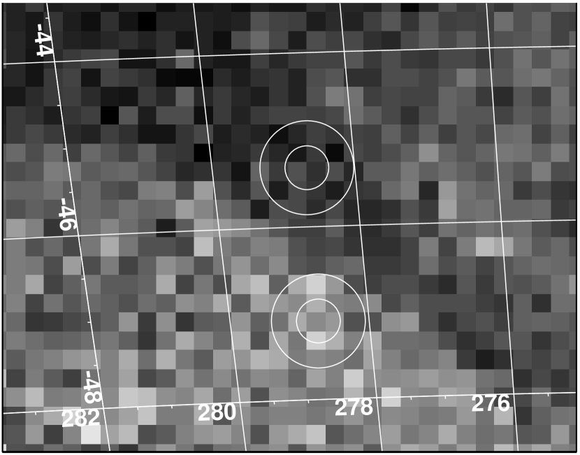
Figure 1.— ROSAT All-Sky Survey R1$+$R2 image centered on $l=279\arcdeg$, $b=-46\arcdeg$, showing the absorbing filament used for our observations (data from Snowden et al., 1997). The circles show our on-filament (upper) and off-filament (lower) pointing directions. The smaller circles ($\mathrm{radius}=14\arcmin$) show the approximate areas from which our XMM-Newton spectra were extracted, while the larger circles ($\mathrm{radius}=30\arcmin$) show the areas from which our ROSAT spectra were extracted.

2. OBSERVATIONS AND DATA REDUCTION

The on- and off-filament XMM-Newton observations were both carried out on 2002 May 3. The details of the observations are presented in Table 1.

Table 1Details of the XMM-NEWTON observations

	Observation	$l$	$b$	Nominal exposure	Usable exposure	$I_{100}$	$N_{\mathrm{H}}$
Observation	ID	(deg)	(deg)	(ks)	(ks)	(MJy $\mbox{sr}^{-1}$)	($10^{20}$ $\mbox{cm}^{-3}$)
On filament	0084960201	278.67	$-45.32$	12.8	11.9	7.10	9.6
Off filament	0084960101	278.73	$-47.09$	27.8	4.4	1.22	1.9

Since our current understanding of the particle background of the XMM-Newton PN is relatively poor, and the characterization of the background of the XMM-Newton MOS cameras is fairly well refined, we have restricted our analysis to the data obtained by the two MOS cameras. The data were reduced as follows. We constructed the light curve in the 2.5–8.5 keV band for the entire field of view. We fitted a Gaussian to a histogram of the count rates, and set the “quiescent level” to the mean of that Gaussian. We removed from further analysis all time periods during which the count rate was $>$$3\sigma$ above the quiescent level; the higher count rate in those time periods is due to either strong soft proton contamination or an enhanced particle background. Filtering the data using a lower-energy band (0.4–2.0 keV) produces results no different from those obtained using the above energy band.

Sources were detected in both the 0.3–2.0 keV and 2.0–10.0 keV bands. Sources with a maximum likelihood detection value greater than 40 (corresponding to $\sim$$10^{-13}$ erg $\mbox{cm}^{-2}$ $\mbox{s}^{-1}$) were removed. The region removed for each source was a circle whose radius contained 80% of the total flux of a point source at the source’s distance from the optical axis; this radius was typically 24–29 arcseconds. The few remaining faint point sources are likely to be background AGN with a power-law spectrum which is unlikely to confuse our analysis of thermal spectra. The actual spectrum of the diffuse emission was extracted from a region with a radius of 14$\arcmin$ approximately centered on the optical axis after the removal of the point sources.

We constructed the spectrum of the “quiescent particle background” from the “unexposed corner” data and filter-wheel-closed data (see Snowden et al., 2004). For each of our two observations, and for each MOS camera, the background spectrum is modeled using a database of filter-wheel-closed data, scaled by data from the unexposed corners of the CCDs of that particular camera. This scaling is energy dependent, and is based upon the hardness and intensity of the unexposed corner data (which varies with time). The background spectrum is interpolated over the 1.2–1.9 keV interval before being subtracted from the observed spectrum. This region of the spectrum contains two bright instrumental lines due to aluminum and silicon (at $\sim$1.48 and $\sim$1.74 keV, respectively). In most of the spectral fits described below, this region of the spectrum was simply excluded. However, leaving the instrumental lines in the observed spectrum and fitting them with Gaussians during the analysis does not significantly affect our results.

The strength of the residual soft proton flares is not known a priori, but the shape is reasonably well modeled by a broken power-law with a break energy of 3.2 keV, where the spectrum is convolved with the redistribution matrix but not scaled by the response function. The contribution of the residual soft proton flares is fitted during the analysis.

2.1. Solar Wind Charge Exchange

The solar wind was very steady during both of these observations. The solar proton flux, measured with the Advanced Composition Explorer (ACE), was $\sim$$1.8\times 10^{8}$ $\mbox{cm}^{-2}$ $\mbox{s}^{-1}$, slightly below the mean, and the proton speed was 420–440 km $\mbox{s}^{-1}$, slightly above the mean. The O⁺⁷/O⁺⁶ and O⁺⁸/O⁺⁷ ratios had typical values. Both observations were taken at a solar angle of $\sim$$80^{\circ}$, avoiding the highest density portions of the magnetosheath. Thus, any solar wind charge exchange (SWCX) contamination will be relatively low and, more to the point, similar for the two observations.

3. SPECTRAL MODELING

3.1. Spectral Model Description

The basic model we used to fit to our XMM-Newton spectra is based upon that used by Snowden et al. (2000) and Kuntz & Snowden (2000) in their analyses of RASS data (which is itself a development of the model used by Snowden et al., 1998). Thus, we use a thermal plasma model in collisional ionization equilibrium (CIE) for the Local Bubble emission. For the Galactic halo emission we use two thermal plasma components (2$T$), and for the extragalactic background (due to unresolved AGN) we use a power-law. In this model, the Local Bubble component is unabsorbed, while the non-local components (halo and extragalactic) are all subject to absorption.

We carried out our spectral fitting with XSPEC v11.3.2p (Arnaud, 1996). Our primary analysis was done using the Astrophysical Plasma Emission Code (APEC) v1.3.1 (Smith et al., 2001) for the thermal plasma components. For comparison, we also analyzed the spectra using the MeKaL model (Mewe et al., 1995), as discussed in §5.4. For the absorption we used the phabs model, which uses cross-sections from Bałucińska-Church & McCammon (1992), except for He, in which case the cross-section from Yan et al. (1998) is used. Our basic XSPEC model was thus $\mathtt{apec}+\mathtt{phabs}\ast(\mathtt{apec}+\mathtt{apec}+\mathtt{powerlaw})$. For chemical abundances we used the interstellar abundance table in Wilms et al. (2000). These abundances were used both by the thermal plasma components and by the absorption model.

The normalization and the photon index of the power-law used to model the extragalactic background were frozen at $10.5(E/\mbox{keV})^{-1.46}$ photons $\mbox{cm}^{-2}$ $\mbox{s}^{-1}$ $\mbox{sr}^{-1}$ $\mbox{keV}^{-1}$ (Chen et al., 1997; from their model A fit to ASCA and ROSAT data). Note that these values were obtained by Chen et al. (1997) after removing point sources down to $\sim$$5\times 10^{-14}$ erg $\mbox{cm}^{-2}$ $\mbox{s}^{-1}$, which is roughly equal to the limit to which we have removed sources (see §2). This means that their result should be applicable to our analysis. Furthermore, the exact values used for the extragalactic power-law have little impact on the fitting of the thermal emission.

We simultaneously analyzed the on- and off-filament spectra. In the fits the temperatures and normalizations of all three apec components were free to vary, but were constrained to be the same for all spectra. The only difference in the model as applied to the different spectra was that the on- and off-filament spectra had different values of $N_{\mathrm{H}}$ for the phabs model. To determine $N_{\mathrm{H}}$ for our two pointing directions, we obtained the 100-µm intensities for these directions from the all-sky IRAS maps of Schlegel et al. (1998) and converted them to $N_{\mathrm{H}}$ using the conversion relation for the southern Galactic hemisphere given in Snowden et al. (2000). The resulting on- and off-filament column densities are $9.6\times 10^{20}$ and $1.9\times 10^{20}$ $\mbox{cm}^{-2}$, respectively (see Table 1). Note that the on-filament column density is consistent with that derived from the color excess of the filament $E(B-V)=0.17\pm 0.05$ (Penprase et al., 1998), which yields $N_{\mathrm{H}}=(8.4\pm 2.5)\times 10^{20}$ $\mbox{cm}^{-2}$ when scaled using the conversion relation in Diplas & Savage (1994). Also, our results are not very sensitive to the values of $N_{\mathrm{H}}$ used.

It should be noted that our absorbing columns do not take into account any contribution from the warm ionized gas in the Reynolds layer, above the disk of the Galaxy. The average column density of this gas is $7\times 10^{19}/\sin|b|$ H ii $\mbox{cm}^{-2}$ (Reynolds, 1991), which gives 9.6–$9.8\times 10^{19}$ H ii $\mbox{cm}^{-2}$ for our observing directions. For 1/4-keV X-rays, the effective absorption cross-section per hydrogen nucleus of the ionized gas is 62% of that for neutral gas (Snowden et al., 1994), which means that at low energies the Reynolds layer would effectively contribute an extra $6\times 10^{19}$ $\mbox{cm}^{-2}$ to our absorbing columns. However, we find that adding this extra contribution to our absorbing columns affects only the cooler halo component, and this has no effect on our conclusions. Furthermore, observations of the Galactic absorption towards extragalactic X-ray sources are generally best fit without the Reynolds layer contribution (e.g. Arabadjis & Bregman, 1999). We therefore proceed using the IRAS-derived column densities quoted above.

As stated in §2, we also included a broken power-law component in our fit to model the contribution of residual soft proton flares not removed in the data reduction. This soft proton contamination evidenced itself in certain XMM-Newton spectra as excess emission above that expected from the extragalactic background power-law at energies $\gtrsim 2$ keV. The broken power-law parameters were the same for the MOS1 and MOS2 spectra for a given pointing, but were allowed to differ between the two pointings.

We also experimented with variants of our “standard” model. One variation used a non-equilibrium ionization (NEI) model for the Local Bubble component, i.e. we replaced the first apec in our model with the XSPEC nei model. In this model, the emitting plasma is assumed to have been rapidly heated to some temperature $T$, but the ionization balance does not yet reflect this new temperature (the ions are underionized). Such a model may be characterized by an ionization parameter, $\tau=n_{\mathrm{e}}t$, where $n_{\mathrm{e}}$ is the electron density and $t$ is the time since the heating. Collisional ionization equilibrium is reached when $\tau\gtrsim 10^{12}$ $\mbox{cm}^{-3}$ s (Masai, 1994). The nei model is configured to use the Astrophysical Plasma Emission Database (APED) to calculate the line spectrum.

Another variation replaced the $2T$ halo model with a model that used a power-law differential emission measure (DEM) of the form

$$\frac{\mathrm{d}(\mbox{E.M.}[T])}{\mathrm{d}(\log T)}\propto\begin{cases}\left(\frac{T}{T_{\mathrm{max}}}\right)^{\alpha}&\text{if $T_{\mathrm{min}}<T<T_{\mathrm{max}}$,}\\ 0&\text{otherwise.}\end{cases}$$ (1)

Here the exponent $\alpha$ and the high-temperature cut-off $T_{\mathrm{max}}$ are free parameters. The low-temperature cut-off is frozen at $T_{\mathrm{min}}=10^{5}$ K (the results are not very sensitive to the value of $T_{\mathrm{min}}$, as plasma at this low a temperature does not significantly contribute to the observed X-ray emission). This model is based upon the XSPEC cemekl model, though we modified it to use APEC instead of MeKaL. The advantage of this model is that it should give a more accurate picture of the temperature distribution of the gas in the Galactic halo. On the other hand, the $2T$ halo model enables an easier comparison with the earlier ROSAT results.

A final variation of our “standard” model was to investigate the effect of varying the abundances of various elements.

We simultaneously analyzed the MOS1 and MOS2 spectra obtained from the on- and off-filament pointings. We used the data between 0.45 and 5 keV, except for the region between 1.2 and 1.9 keV, where there are two bright instrumental lines (see §2). An alternative to excluding these data is to fit these two lines by adding two Gaussians to the model; however, as stated in §2, there is no significant difference between the results obtained in these two ways.

In order to better constrain the models at softer energies, we also included two ROSAT spectra in the fits. These were extracted from ROSAT All-Sky Survey data (Snowden et al., 1997) using the HEASARC X-ray Background Tool v2.3. The spectra were extracted from 0.5° radius circles centered on the two XMM-Newton pointing directions, and are normalized to one square arcminute. While larger circles would have reduced the errors on the ROSAT data, they would result in the on-filament ROSAT spectrum being contaminated by off-filament emission, and vice versa (see Fig. 1).

We accounted for the difference between the XMM-Newton effective field of view and the solid angle used in the ROSAT extraction by multiplying the model applied to the XMM-Newton data by the XMM-Newton field of view ($\sim$580 arcmin²), and normalizing the ROSAT spectra to 1 arcmin², as mentioned above.

After our fitting was complete, we converted the XSPEC model normalizations to emission measures ($\int n_{\mathrm{e}}^{2}\mathrm{d}l$) assuming $n_{\mathrm{He}}/n_{\mathrm{H}}=0.1$, and neglecting the contribution of metals to the electron density $n_{\mathrm{e}}$.

3.2. A Note on the Abundance Table Used

As stated in the previous section, we used the Wilms et al. (2000) interstellar abundances, which differ from those in widely used solar abundance tables (e.g. Anders & Grevesse, 1989; Grevesse & Sauval, 1998) for many astrophysically abundant elements. For example, Wilms et al. (2000) give an interstellar oxygen abundance $n_{\mathrm{O}}/n_{\mathrm{H}}=4.90\times 10^{-4}$, compared with solar abundances of $8.51\times 10^{-4}$ (Anders & Grevesse, 1989) or $6.76\times 10^{-4}$ (Grevesse & Sauval, 1998). However, more recent measurements of the solar photospheric oxygen abundance (Allende Prieto et al., 2001; Asplund et al., 2004) are in excellent agreement with the Wilms et al. (2000) value. Indeed, recent measurements of other metals’ photospheric abundances (e.g. C, N, Fe; Asplund et al., 2005) are lower than the Anders & Grevesse (1989) and Grevesse & Sauval (1998) values, and are in better agreement with the Wilms et al. (2000) values. Therefore, in this paper we take the Wilms et al. (2000) interstellar abundances to be synonymous with solar abundances.

4. RESULTS

4.1. Spectral Fit Results

The results of fitting the above-described “standard” ($2T$ halo) model are presented in Table 2. Also shown in this table are the results of using the XSPEC non-equilibrium nei model for the Local Bubble, and of using a power-law differential emission measure (DEM) for the halo emission (see eq. [1]). When we tried varying various chemical abundances, we found that the deviations from solar abundances were either statistically insignificant or inconsistent (e.g. the Local Bubble oxygen abundance was somewhat dependent upon the halo model used). We therefore do not present any non-solar-abundance results in Table 2, and for the remainder of this paper we just discuss our solar-abundance results.

Table 2Spectral fit results

					$2T$ halo model
	Local Bubble				Halo (cool)			Halo (hot)
	$\log T$	E.M.	$\tau$		$\log T$	E.M.		$\log T$	E.M.
Model	(K)	($\mbox{cm}^{-6}$ pc)	($10^{10}$ $\mbox{cm}^{-3}$ s)		(K)	($\mbox{cm}^{-6}$ pc)		(K)	($\mbox{cm}^{-6}$ pc)	$\chi^{2}/\mbox{dof}$
“Standard” (CIE Local Bubble)	$6.06^{+0.02}_{-0.04}$	0.018	$\cdots$		$5.93^{+0.04}_{-0.03}$	0.17		$6.43\pm 0.02$	0.011	$435.86/439$
NEI Local Bubble	$6.21^{+0.08}_{-0.10}$	0.011	$3.4^{+4.7}_{-1.4}$		$5.90^{+0.02}_{-0.03}$	0.22		$6.44\pm 0.02$	0.010	$434.56/438$
No Local Bubble	$\cdots$	$\cdots$	$\cdots$		$5.92\pm 0.01$	0.37		$6.44\pm 0.02$	0.012	$801.12/441$
One halo component	$6.05^{+0.01}_{-0.02}$	0.023	$\cdots$		$\cdots$	$\cdots$		$6.37\pm 0.01$	0.018	$539.57/441$
Hot Local Bubble	6.21 (frozen)	0.017	$\cdots$		$5.29^{+0.13}_{-0.08}$	160		$6.49\pm 0.02$	0.0073	$444.04/440$
	Local Bubble					DEM halo model
	$\log T$	E.M.	$\tau$			$\log T_{\mathrm{max}}$		$\alpha$
Model	(K)	($\mbox{cm}^{-6}$ pc)	($10^{10}$ $\mbox{cm}^{-3}$ s)			(K)				$\chi^{2}/\mbox{dof}$
CIE Local Bubble	$6.02^{+0.01}_{-0.02}$	0.018	$\cdots$			$6.70\pm 0.07$		$-2.01^{+0.14}_{-0.13}$		$438.62/440$
No Local Bubble	$\cdots$	$\cdots$	$\cdots$			$>$6.80		$-2.73^{+0.08}_{-0.07}$		$801.64/442$

Note from Table 2 that the Local Bubble model parameters do not significantly change whether one uses a $2T$ or power-law DEM model for the halo. For completeness we show the halo emission measure given by the power-law DEM model in Figure 2, but as this paper is mainly concerned with the Local Bubble, we defer discussion of the halo results to a later paper. For the remainder of this paper the results discussed will be those obtained with the $2T$ halo model.

The spectra and the best-fit “standard” model are shown in Figure 3. Note the offset between the total model emission and the extragalactic component above $\sim$2 keV in the off-filament XMM-Newton data. This is entirely due to soft-proton contamination (see §3.1). Note also that in the XMM-Newton band the Local Bubble component makes a significant contribution only to the O vii emission at $\sim$0.57 keV. Most ($\sim$90%) of the O viii emission at $\sim$0.65 keV is due to the hotter halo component, with the extragalactic background contributing $\sim$8% of the emission at this energy. However, the Local Bubble dominates the spectrum at the lowest energies in the on-filament ROSAT spectrum, as the halo and extragalactic components are very strongly absorbed. The absorbing cross-section per hydrogen atom is $8.96\times 10^{-21}$ $\mbox{cm}^{2}$ at 0.2 keV, calculated using the Bałucińska-Church & McCammon (1992) cross-sections (except for He; Yan et al., 1998) with the Wilms et al. (2000) interstellar abundances. This gives an on-filament optical depth of 8.6 at this energy.

While there are some features that are poorly fit in one of the spectra (e.g. the model underestimates the O vii emission in the off-filament MOS1 spectrum), when one considers all the spectra together there are no features that are systematically poorly fit. Overall, the model gives a good fit to the data, with $\chi^{2}_{\nu}=0.99$ for 439 degrees of freedom.

We tested whether or not a Local Bubble component is necessary by trying a model without a Local Bubble component. As can be seen from Table 2 such a model gives a poor fit to the data whether one uses a $2T$ model ($\chi^{2}_{\nu}=1.82$ for 441 degrees of freedom) or a power-law DEM model ($\chi^{2}_{\nu}=1.81$ for 442 degrees of freedom) for the halo. As can also be seen from the table, a $1T$ halo model gives a poor fit to the data ($\chi^{2}_{\nu}=1.22$ for 441 degrees of freedom).

Figure 2.— Our best-fitting halo power-law differential emission measure (DEM) model. The two arrows mark the temperatures obtained from the $2T$ halo model.

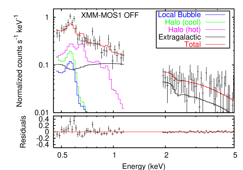
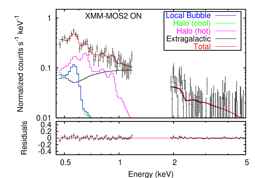
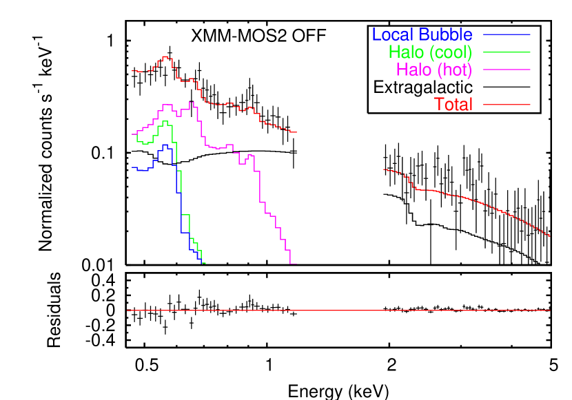
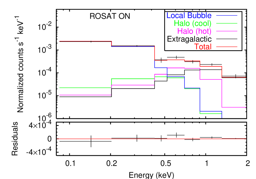
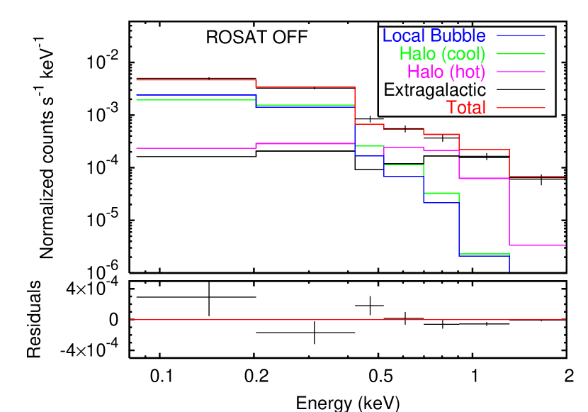
Figure 3.— Our observed on-filament (left-hand column) and off-filament (right-hand column) spectra, with our best-fit “standard” model (note the different energy ranges on the XMM-Newton and ROSAT plots). The individual components that comprise our model are also illustrated. Note in the on-filament XMM-Newton results that the Local Bubble (blue) and cool halo (green) components overlap. The gap in the XMM-Newton data is where two bright instrumental fluorescence lines have been excluded. The large difference between the XMM-Newton and ROSAT count-rates is because the ROSAT data have been normalized to one square arcminute, whereas the XMM-Newton data are integrated over the illuminated XMM-Newton field of view ($\approx$580 arcmin²).

4.2. Local Bubble O VII and O VIII Intensities

To measure the intensities of the O vii and O viii emission from the Local Bubble, we replaced the Local Bubble apec component in our “standard” model with a $\mathtt{gaussian}+\mathtt{gaussian}+\mathtt{vapec}$ model, with the oxygen abundance of the vapec component frozen at zero. The two Gaussians model the oxygen line emission, while the vapec component models the continuum and the contribution of other lines. The widths of the Gaussians were fixed at zero, and the energies were fixed at 0.5681 and 0.6536 keV for O vii and O viii, respectively. For O vii this is the mean energy of the resonance, intercombination, and resonance lines, weighted by the line emissivities for a $10^{6.06}$ K plasma. For O viii it is the weighted mean energy of the two Ly$\alpha$ lines. The relevant line energies and emissivities were obtained from the APEC code using the XSPEC identify command. Thawing the energies of the Gaussians did not significantly improve the fit, nor did it significantly alter the measured intensities. The temperature and normalization of the Local Bubble vapec component were allowed to vary, while the parameters of all the other components were held fixed at their best-fit values from the previous section.

We fit this new model to our on- and off-filament XMM-Newton and ROSAT spectra, as before. We measure an O vii intensity of $3.4^{+0.6}_{-0.4}$ photons $\mbox{cm}^{-2}$ $\mbox{s}^{-1}$ $\mbox{sr}^{-1}$, and obtain a $3\sigma$ upper limit on the O viii intensity of 1.0 photons $\mbox{cm}^{-2}$ $\mbox{s}^{-1}$ $\mbox{sr}^{-1}$ (see Table 3). We use these results in §5.6.

We can check these values using line emissivity data from the ATOMDB database. The temperature and emission measure of our “standard” model Local Bubble component yield O vii and O viii intensities of 2.9 and 0.017 photons $\mbox{cm}^{-2}$ $\mbox{s}^{-1}$ $\mbox{sr}^{-1}$, respectively, including the contribution of dielectronic recombination satellite lines. These values are consistent with the above-measured values. Although the O vii intensity measured from the Gaussian fits is higher than that obtained from ATOMDB, this is unlikely to be due to contamination by other oxygen lines, as there are no other bright oxygen lines in that vicinity. Instead, it is possible that the Local Bubble apec model is slightly underestimating the contribution of the Local Bubble to the observed O vii emission. This is because this component is not being constrained solely by the oxygen emission, but also by emission at other energies (e.g. the ROSAT R12 intensity and the R1/R2 ratio). The O viii emission is more likely to be contaminated, for example by O vii $n=3\rightarrow 1$ emission at 0.6656 keV. However, this just means that the above upper limit may be overly conservative; it does not adversely affect our later analysis and conclusions.

McCammon et al. (2002) measured the intensities of O vii and O viii in the soft X-ray background using the X-ray Quantum Calorimeter (XQC), which was flown on a sounding rocket. They obtained intensities of $4.8\pm 0.8$ and $1.6\pm 0.4$ photons $\mbox{cm}^{-2}$ $\mbox{s}^{-1}$ $\mbox{sr}^{-1}$ for O vii and O viii, respectively. These are total intensities for the soft X-ray background averaged over a large area of sky ($\sim$1 sr), whereas the intensities in Table 3 are just for the Local Bubble. Our results are therefore consistent with the McCammon et al. (2002) results.

Table 3Local Bubble O vii and O viii intensities

	Energy	Intensity
Ion	(keV)	(photons $\mbox{cm}^{-2}$ $\mbox{s}^{-1}$ $\mbox{sr}^{-1}$)
O vii	0.5681	$3.4^{+0.6}_{-0.4}$
O viii	0.6536	$<1.0$

4.3. Derived Parameters of the Local Bubble

If we assume some spatial extent $L$ for the Local Bubble in our pointing direction, and assume that the Local Bubble plasma is uniform along the line of sight, we can convert the emission measure found above to a density. With the measured plasma temperature, this will give us the thermal pressure of the plasma. If we make the further simplifying assumption that the Local Bubble is a sphere of radius $L$, we can estimate the thermal energy content and the cooling time of the Local Bubble.

The Local Bubble parameters derived from the “standard” model parameters in Table 2 are shown in Table 4.

Table 4Derived parameters of the Local Bubble

Parameter	Value
Electron density $n_{\mathrm{e}}$ ($\mbox{cm}^{-3}$)	$0.013(L/100~{}\mbox{pc})^{-1/2}$
Number density $n$ ($\mbox{cm}^{-3}$)	$0.026(L/100~{}\mbox{pc})^{-1/2}$
Pressure $p/k$ ($\mbox{cm}^{-3}$ K)	$2.9\times 10^{4}(L/100~{}\mbox{pc})^{-1/2}$
Thermal energy $E_{\mathrm{th}}$ (erg)	$7.4\times 10^{50}(L/100~{}\mbox{pc})^{5/2}$
Cooling time $t_{\mathrm{cool}}$ (yr)	$1.7\times 10^{7}(L/100~{}\mbox{pc})^{1/2}$
Sound crossing time $t_{\mathrm{cross}}$ (yr)	$1.2\times 10^{6}(L/100~{}\mbox{pc})$

Note. — Calculated from the “standard” model parameters for the Local Bubble in Table 2, assuming the radius of the Local Bubble is $L$.

5. DISCUSSION

In this section, we first compare our results with the results of analyses of ROSAT All-Sky Survey (RASS) data in §5.1. In §5.2 we discuss our results in terms of the Galactic halo O vi emission (R. L. Shelton et al., in preparation). We compare our results with those of other XMM-Newton and Chandra shadowing observations of the Local Bubble in §5.3. We find a discrepancy between our Local Bubble temperature and that measured by other XMM-Newton observations, and discuss whether or not this can be attributed to our choice of plasma emission code in §5.4. Finally we discuss non-equilibrium models of the Local Bubble: in §5.5 we discuss the results of using an underionized (ionizing) model of the Local Bubble (i.e. the XSPEC nei model), and in §5.6 we discuss our results in terms of an overionized (recombining) model of the Local Bubble.

5.1. Comparison with ROSAT Results

In Table 5 we compare our measured temperatures with those measured in various studies of RASS data. As can be seen, there is excellent agreement between our values and the ROSAT-determined values. This is not surprising, as we use RASS data to constrain our spectral models at low energies. However, our Local Bubble emission measure ($\int n_{\mathrm{e}}^{2}\mathrm{d}l=0.018$ $\mbox{cm}^{-6}$ pc) is 3–10 times larger than that derived from the ROSAT data (0.0018–0.0058 $\mbox{cm}^{-6}$ pc; Snowden et al., 1998).

This discrepancy is due to the fact that Snowden et al. (1998) use the Raymond & Smith (1977) plasma emission code, whereas we use APEC. Also, Snowden et al. (1998) assume a higher metallicity in their study: $Z=0.017$ (Allen, 1973) against $Z=0.012$ (Wilms et al., 2000). For a $T=10^{6.06}$ K plasma, a Raymond & Smith model with $Z=0.017$ predicts $\sim$3 times as much flux in the 0.1–0.5 keV band as an APEC model with $Z=0.012$. Hence, for a given amount of Local Bubble emission, our model will give an emission measure $\sim$3 times larger than Snowden et al.’s (1998) model, which is what we find.

Table 5Comparison with ROSAT results

	$\log T_{\mathrm{LB}}$	$\log T_{\mathrm{Halo,1}}$	$\log T_{\mathrm{Halo,2}}$
Work	(K)	(K)	(K)
Snowden et al. (1998)	$6.07\pm 0.05$	$6.02\pm 0.08$	$\cdots$
Snowden et al. (2000)	6.08	6.00	6.4
Kuntz & Snowden (2000)	$6.11^{+0.15}_{-0.07}$	$6.06^{+0.19}_{-0.20}$	$6.46^{+0.12}_{-0.08}$
This work	$6.06^{+0.02}_{-0.04}$	$5.93^{+0.04}_{-0.03}$	$6.43\pm 0.02$

5.2. The Galactic Halo O VI Emission

As already stated, the main focus of this paper is the Local Bubble emission, with discussion of the Galactic halo emission being deferred to a later paper. However, we note here that our fit results may also be used to make predictions of the halo O vi intensity, which may then be compared with that measured from an off-filament Far Ultraviolet Spectroscopic Explorer (FUSE) observation. This provides a useful check on our fit results.

Assuming all the halo O vi emission originates from beyond the absorbing material in that direction (which has a transmissivity to O vi photons of 58%), the intrinsic intensity of the doublet is $8070^{+980}_{-1140}$ photons $\mbox{cm}^{-2}$ $\mbox{s}^{-1}$ $\mbox{sr}^{-1}$ (R. L. Shelton et al., in preparation). In comparison, the best-fit temperature and emission measure of the cooler halo component from our “standard” model predicts an intrinsic O vi doublet intensity of $\sim$3000 photons $\mbox{cm}^{-2}$ $\mbox{s}^{-1}$ $\mbox{sr}^{-1}$ (using data from the ATOMDB database). Here we use the $2T$ halo model, as the halo differential emission measure is poorly constrained at low temperatures. Furthermore, we just consider the cooler halo component, as the contribution of the hotter component to the O vi emission is negligible.

We used a Monte Carlo method to estimate the uncertainty on this O vi intensity prediction. We generated 1000 random pairs of ($T$ [halo], E.M. [halo]), where $\mbox{E.M.~{}[halo]}=\int n_{\mathrm{e}}^{2}\mathrm{d}l$ is the emission measure of the cooler halo component. These pairs of numbers were drawn at random from normal distributions whose standard deviations are given by the errors on the measured parameters in Table 2 ($\mbox{E.M. [halo]}=0.17^{+0.05}_{-0.04}$ $\mbox{cm}^{-6}$ pc), and were used to calculate 1000 values of the O vi doublet intensity. We fit a Gaussian to the distribution of these values, and from the mean and standard deviation obtain a predicted O vi intensity of $3100\pm 1000$ photons $\mbox{cm}^{-2}$ $\mbox{s}^{-1}$ $\mbox{sr}^{-1}$ (see Fig. 4). The observed intensity is $3.3\sigma$ larger than the predicted intensity (though the distribution of predicted intensities is positively skewed, which will tend to reduce the significance of this difference). These results indicate that there is more O vi in the halo than is expected from the hot gas alone. This is probably because O vi can also arise in the warm interfaces between cool clouds and the hot gas.

Figure 4.— Histogram of 1000 randomly generated values of the intrinsic Galactic halo O vi intensity, predicted from our measured values of the halo temperature and emission measure, taking into account the errors on these parameters. The arrow and the horizontal bar denote the intrinsic intensity inferred from FUSE, assuming all the O vi emission originates from beyond the absorbing material in that direction (see text for details).

5.3. Comparison with Other Shadowing Observations of the Local Bubble

XMM-Newton has been used to make shadowing observations of the Local Bubble in the directions of the MBM 12 and Ophiuchus molecular clouds (Freyberg & Breitschwerdt, 2003; Freyberg, 2004), and in the direction of the Bok globule Barnard 68 (Freyberg et al., 2004). Chandra has also been used to observe MBM 12 (Smith et al., 2005).

The Local Bubble temperatures inferred from these XMM-Newton observations are consistently higher than the temperature we measure: $\log(T_{\mathrm{LB}}/\mathrm{K})=6.21^{+0.06}_{-0.07}$ for MBM 12 and Ophiuchus (Freyberg & Breitschwerdt, 2003; Freyberg, 2004) and $\log(T_{\mathrm{LB}}/\mathrm{K})\approx 6.24$ for Barnard 68 (see Appendix), versus $\log(T_{\mathrm{LB}}/\mathrm{K})=6.06^{+0.02}_{-0.04}$ from our data. Note, however, that for MBM 12 there is an additional $\log(T/\mathrm{K})\approx 6$ component (Freyberg, 2004). It should also be noted that Freyberg & Breitschwerdt (2003) and Freyberg (2004) do not state whether or not they use ROSAT data to constrain their fits at lower energies.

In contrast to these XMM-Newton results, Smith et al. (2005) found that they could not explain the O vii:O viii ratio in their Chandra observation of MBM 12 with an equilibrium Local Bubble model with $\log(T_{\mathrm{LB}}/\mathrm{K})<6.3$. However, they do note the possibility that their O viii emission is contaminated by emission from another source, such as solar charge exchange emission.

These other shadowing observations were carried out using much thicker absorbers than our observations: $4\times 10^{21}$ $\mbox{cm}^{-2}$ for MBM 12 (Smith et al., 2005) up to $\sim$$10^{23}$ $\mbox{cm}^{-2}$ for Barnard 68 (Freyberg et al., 2004), against $9.6\times 10^{20}$ $\mbox{cm}^{-2}$ for our filament. The optical depth at O viii energies is at least 2 for these other observations, implying a transmissivity for background O viii radiation of less than 14%. In an observation of one of these thicker absorbers, one may confidently attribute a large fraction of any observed O viii emission to the foreground, and thus infer a higher Local Bubble temperature. However, the higher transmissivity of our filament (61% at O viii energies) makes it harder to determine how much of the observed emission is from the Local Bubble, and how much is background emission that has leaked through the filament. Our best-fit “standard” model attributes only $\sim$2% of the observed on-filament O viii emission to the Local Bubble, compared with $\sim$30% of the observed O vii emission. The fact that our best-fit model attributes so little O viii emission to the Local Bubble leads to our lower value of $T_{\mathrm{LB}}$. However, the question remains, could more of the O viii emission in our observation be due to the Local Bubble? To put this more precisely, are our data also consistent with $\log(T_{\mathrm{LB}}/\mathrm{K})=6.21$?

We tested this by re-fitting our “standard” model to the data, but with $T_{\mathrm{LB}}$ frozen at $10^{6.21}$ K. The results of this are shown in Table 2. This model does give a good fit to the data ($\chi^{2}_{\nu}=1.01$ for 440 degrees of freedom). However, note that the temperature of the cooler halo component has significantly decreased, and its emission measure has increased by three orders of magnitude. Both these effects lead to a huge increase in the predicted intrinsic halo O vi intensity (cf. §5.2) to $\sim$$10^{7}$ photons $\mbox{cm}^{-2}$ $\mbox{s}^{-1}$ $\mbox{sr}^{-1}$. As before, we used a Monte Carlo method to estimate the uncertainty on this prediction. In this case, there is a much larger error on the emission measure of the cooler halo component ($\mbox{E.M. [halo]}=160^{+1000}_{-20}$ $\mbox{cm}^{-6}$ pc), resulting in a much larger dynamic range in the predicted intensities. By fitting a Gaussian to the distribution of the logarithms of the predicted values, we find the predicted intensity is $\log(I_{\mathrm{O\,VI}}/\mathrm{ph}\ \mbox{cm}^{-2}\ \mbox{s}^{-1}\ \mbox{sr}^{-1})=7.5\pm 1.1$. In comparison, the intrinsic intensity inferred from the FUSE data is $\log(I_{\mathrm{O\,VI}}/\mathrm{ph}\ \mbox{cm}^{-2}\ \mbox{s}^{-1}\ \mbox{sr}^{-1})=3.79^{+0.05}_{-0.06}$ (R. L. Shelton et al., in preparation). While we could interpret the discrepancy between the predicted and observed intensities as evidence that the Galactic halo is out of equilibrium, given the size of the discrepancy (i.e. possibly up to a few orders of magnitude), we instead interpret it as evidence that $\log(T_{\mathrm{LB}}/\mathrm{K})=6.21$ is inconsistent with our XMM-Newton spectra and the FUSE results when taken together.

It should be noted that two of the clouds discussed above (Ophiuchus and Barnard 68) lie beyond the Local Bubble in the direction of Loop I, near the Galactic plane. It is therefore possible that the foreground emission (which in the above discussion we have attributed to the Local Bubble) is being contaminated by emission from Loop I. However, Freyberg (2004) states that the weakness of the Fe-L line emission (attributed to Loop I) in the on-cloud Ophiuchus spectrum indicates that the contamination is small. In contrast to this, MBM 12 does not lie towards any obvious source of contamination, and may even lie within the Local Bubble, implying that the temperature inferred from these observations is indeed that of the Local Bubble.

Our pointing direction is $\gtrsim 80^{\circ}$ away from the directions of the other XMM-Newton observations. It is therefore not implausible that our value of $T_{\mathrm{LB}}$ is different from those measured from these observations, as we are observing a different part of the Local Bubble. These results therefore suggest that the Local Bubble is thermally anisotropic.

5.4. Choice of Plasma Emission Code

In this section we consider what effect, if any, the choice of plasma emission code used has on the measured Local Bubble temperature.

The higher foreground temperatures measured from the XMM-Newton spectra of MBM 12, the Ophiuchus molecular cloud, and Barnard 68 should be quite robust, regardless of the plasma emission code used. This is because O viii emission is observed towards these clouds. Due to the large optical depths of the clouds, a large fraction of this emission may be attributed to the foreground, implying a higher temperature than we found towards our filament. Freyberg & Breitschwerdt (2003) do not give details of the models used in their analysis of the XMM-Newton observations of MBM 12 and Ophiuchus, but they do note that $\log(T_{\mathrm{LB}}/\mathrm{K})=6.21^{+0.06}_{-0.07}$ “or higher, depending on the actual model.” Also, we infer $\log(T_{\mathrm{LB}}/\mathrm{K})=6.24$ from Freyberg et al.’s (2004) Barnard 68 data whether we use APEC or MeKaL (see Appendix). However, since our filament is less optically thick than these other clouds, there is a greater ambiguity between what is Local Bubble emission and what is halo emission, and so we test the possibility that different codes would attribute different amounts of the emission in our spectra to the Local Bubble and the halo, leading to a different value of $T_{\mathrm{LB}}$.

We tested this by repeating our fits using the MeKaL code instead of APEC for the thermal emission components. The results are compared with our APEC results in Table 6. Note in particular that MeKaL gives a higher Local Bubble temperature than APEC: $\log(T_{\mathrm{LB}}/\mathrm{K})=6.17^{+0.06}_{-0.07}$ (MeKaL) versus $6.06^{+0.02}_{-0.04}$ (APEC). It should be emphasized that the difference between the APEC and MeKaL results for our data is not because the two codes give different temperatures for the same Local Bubble spectrum. Instead it is because MeKaL attributes more of the O viii emission to the Local Bubble (see Fig. 5), and correspondingly less to the halo. Hence, the inferred Local Bubble spectrum is different between the two codes, and thus so too is $T_{\mathrm{LB}}$. This discrepancy is most likely to be due to uncertain modeling of the lines from L-shell ions of Ne, Mg, and Si, which dominate the emission at the lowest ROSAT energies. The ATOMDB v1.3.1 release notes contain a caveat that there are very few data on lines from these ions (other than Li-like ions). Differences between the codes in this energy regime would affect the fits to the ROSAT data, which would then affect the fitting to the higher-energy XMM-Newton data.

To test whether or not this does cause the discrepancy between the APEC and MeKaL results, we re-fit our “standard” model just to the XMM-Newton spectra, without the ROSAT data. These results are also shown in Table 6. Note that these temperatures are unphysical, as they are inconsistent with the low-energy ROSAT data. However, the agreement between the codes’ results is much better than before, suggesting that at least part of the discrepancy is due to uncertain modeling of lines in the lowest-energy ROSAT bins.

Despite this discrepancy, we reiterate that the measurement of $\log(T_{\mathrm{LB}}/\mathrm{K})\geq 6.21$ from the other XMM-Newton observations should not be strongly code-dependent, and note that we obtain a lower temperature than this whether we use APEC or MeKaL. This therefore implies that the conclusion of the previous section, namely that the Local Bubble appears to be thermally anisotropic, is not an artefact of our choice of plasma emission code. However, we should reiterate the possibility that the foreground emission in some of the other XMM-Newton observations may be contaminated by non-Local Bubble emission.

Figure 5.— Our best fitting APEC and MeKaL Local Bubble models, folded through the XMM-Newton MOS1 instrumental response. Note that there is more Local Bubble O viii emission at $\sim$0.65 keV in the MeKaL model than in the APEC model.

Table 6Comparison of APEC and MeKaL results

	ROSAT	$\log T_{\mathrm{LB}}$	$\log T_{\mathrm{Halo,1}}$	$\log T_{\mathrm{Halo,2}}$
Code	included?	(K)	(K)	(K)	$\chi^{2}/\mbox{dof}$
APEC	Y	$6.06^{+0.02}_{-0.04}$	$5.93^{+0.04}_{-0.03}$	$6.43\pm 0.02$	$435.86/439$
MeKaL	Y	$6.17^{+0.06}_{-0.07}$	$5.67^{+0.01}_{-0.02}$	$6.35\pm 0.02$	$433.68/439$
APEC	N	$6.44^{+0.03}_{-0.08}$	$6.20^{+0.04}_{-0.11}$	$6.69^{+0.10}_{-0.13}$	$410.21/425$
MeKaL	N	$6.37^{+0.06}_{-0.10}$	$6.21^{+0.13}_{-0.07}$	$6.75^{+0.15}_{-0.20}$	$411.57/425$

5.5. Ionizing Model of the Local Bubble

In the preceding sections we have just discussed collisional ionization equilibrium (CIE) plasma models. In this section we discuss the results of using the XSPEC nei model to model the Local Bubble emission (see Table 2). This is a model in which the ions are underionized, i.e. the plasma has been rapidly heated, but the ionization balance does not yet reflect the new temperature: the ions are still in the process of ionizing. As stated in §3.1, such a model may be characterized by an ionization parameter, $\tau=n_{\mathrm{e}}t$, where $n_{\mathrm{e}}$ is the electron density and $t$ is the time since the heating. Equilibrium is reached when $\tau\gtrsim 10^{12}$ $\mbox{cm}^{-3}$ s (Masai, 1994).

In certain situations one may use the F-test to determine whether or not adding an extra model parameter leads to a significant improvement in $\chi^{2}$ (Bevington & Robinson, 2003). Unfortunately we cannot use the F-test here to test whether or not the non-equilibrium model is an improvement on the equilibrium model. This is because the additional parameter ($\tau$) is on the boundary of the set of possible parameter values in the simpler (null) model (i.e. $\tau=\infty$ in the equilibrium model). In such a case, one cannot use the F-test (Protassov et al., 2002).

However, we can note that the difference in $\chi^{2}$ between the two models is very small, suggesting that thawing $\tau$ does not lead to a significant improvement in $\chi^{2}$ (even if we cannot use the F-test to demonstrate this for certain). On the other hand, it should be noted that the value of $\tau$ we measure ($[3.4^{+4.7}_{-1.4}]\times 10^{10}$ $\mbox{cm}^{-3}$ s) is significantly less than what is expected in the equilibrium case ($\tau\gtrsim 10^{12}$ $\mbox{cm}^{-3}$ s; Masai, 1994), which means that our data cannot rule out an ionizing non-equilibrium model.

In order to distinguish between equilibrium and non-equilibrium models we would require more spectral information. With our data, the only Local Bubble “line” (actually a blend of lines) we can clearly see is the O vii feature at $\sim$0.57 keV. There are no other obvious Local Bubble lines in the XMM-Newton bandpass (the observed O viii feature in the on-filament spectrum is attributed to leak through from the Galactic halo), and we only have two ROSAT spectral bins at energies below the XMM-Newton bandpass. In contrast to this, one needs to compare the flux ratios of lines from several different ions in order to determine whether or not non-equilibrium effects are important.

In principle, we could use data from other wavebands to help distinguish between the two classes of model. FUSE has observed the Local Bubble in the same directions as our XMM-Newton observations. Using the on-filament observation, Shelton (2003) has placed a $2\sigma$ upper limit on the Local Bubble O vi $\lambda\lambda 1032$, 1038 doublet intensity of 800 photons $\mbox{cm}^{-2}$ $\mbox{s}^{-1}$ $\mbox{sr}^{-1}$ (including statistical and systematic uncertainties). In comparison, the predicted O vi intensities of our best-fit models (determined using XSPEC) are 180 photons $\mbox{cm}^{-2}$ $\mbox{s}^{-1}$ $\mbox{sr}^{-1}$ (equilibrium) and 63 photons $\mbox{cm}^{-2}$ $\mbox{s}^{-1}$ $\mbox{sr}^{-1}$ (non-equilibrium), both of which are consistent with the observed upper limits.

We therefore conclude that our data are unable to distinguish between an equilibrium plasma model and a non-equilibrium model in which the ions are underionized and are in the process of ionizing.

5.6. Recombining Model of the Local Bubble

In this section we consider an alternative non-equilibrium Local Bubble model to the previous section, namely one in which the plasma is overionized and the ions are in the process of recombining.

Such a model for the Local Bubble was originally proposed by Breitschwerdt & Schmutzler (1994; see also Breitschwerdt, 1996; Breitschwerdt et al., 1996; Breitschwerdt, 2001). In this model, the Local Bubble is assumed to be the relic of an old superbubble formed by $\sim$10 successive supernovae in a dense ($\sim$$10^{4}$ $\mbox{cm}^{-3}$) molecular cloud. A few million years ago, the bubble burst out of the cloud and underwent rapid adiabatic expansion into the surrounding medium, assumed to be $\sim$10–100 times less dense than the cloud. During this process the bubble adiabatically cooled to $\lesssim 10^{5}$ K (i.e. much less than the temperature inferred from the X-rays assuming collisional ionization equilibrium). However, owing to the rapidity of the cooling, the ions remained in high ionization states. The observed X-rays are then supposed to be due to the delayed recombinations of these overionized ions, rather than being from a hot ($\sim$$10^{6}$ K) plasma in equilibrium.

A recombining plasma model has a number of appealing features. Firstly, there is an order of magnitude difference between the pressure of the Local Cloud in which the solar system resides ($P_{\mathrm{LC}}/k\sim 2000$ $\mbox{cm}^{-3}$ K; Lallement, 1998) and the pressure of the surrounding Local Bubble inferred from the X-ray data assuming CIE ($P_{\mathrm{LB}}/k\sim$ 15,000 $\mbox{cm}^{-3}$ K [Snowden et al., 1998] to 29,000 $\mbox{cm}^{-3}$ K [Table 4]). It is difficult to see how such a large pressure difference can be maintained. The lower Local Bubble temperature in the Breitschwerdt & Schmutzler (1994) model greatly reduces the Local Bubble pressure, and thus eliminates this problem. Secondly, the electron density inferred from the dispersion measure of the pulsar PSR $0950+08$ ($d\approx 130$ pc) is 0.023 $\mbox{cm}^{-3}$ (Reynolds, 1990). If this density is representative of the Local Bubble, then a $\sim$$10^{6}$ K plasma in equilibrium would produce too much X-radiation (cf. the electron density inferred from the X-ray data assuming CIE is $\sim$0.007 $\mbox{cm}^{-3}$ [Snowden et al., 1998] to 0.013 $\mbox{cm}^{-3}$ [Table 4]). However, a higher $n_{\mathrm{e}}$ is acceptable within the Breitschwerdt & Schmutzler (1994) model. Thirdly, a $\sim$$10^{6}$ K plasma in equilibrium should produce most of its emission as lines in the extreme ultraviolet (EUV). However, such emission is not observed. Extreme Ultraviolet Explorer (EUVE) spectra of the diffuse EUV background ($\sim$17–80 eV) place an upper limit on the emission measure of a local $10^{6}$ K plasma which is an order of magnitude less than the Local Bubble emission measures in Table 2 (Jelinksy et al., 1995; Vallerga & Slavin, 1998). A recombining plasma model can explain this observation, as the much lower kinetic temperature suppresses collisional excitation of the EUV lines (Breitschwerdt, 1996).

Here we examine whether or not a recombining plasma model can simultaneously explain our observed Local Bubble O vii intensity and the observed upper limits on the O vi and O viii intensities. We do this by first calculating the fractions of oxygen in the ionization states O vi to O ix, and then using these populations to predict the line intensities. These are then compared with the observed limits. For this purpose we use $3\sigma$ limits. Note that Shelton (2003) does not explicitly quote a $3\sigma$ upper limit for the O vi intensity, but we can obtain one from the data in her Table 2. The $3\sigma$ upper limit on the $\lambda 1032$ intensity obtained from the combined $\mbox{day}+\mbox{night}$ FUSE data is 710 photons $\mbox{cm}^{-2}$ $\mbox{s}^{-1}$ $\mbox{sr}^{-1}$ (statistical uncertainty only). As the theoretical $\lambda 1032$-to-$\lambda 1038$ intensity ratio is 2 to 1, the $3\sigma$ upper limit on the doublet intensity is 1065 photons $\mbox{cm}^{-2}$ $\mbox{s}^{-1}$ $\mbox{sr}^{-1}$.

In a purely recombining plasma (i.e. one in which ionizations can be ignored), the fraction $p_{i}$ of the atoms of a given element in an ionization state with $i$ electrons is given by

$$\frac{\mathrm{d}p_{i}}{\mathrm{d}t}=-R_{i}n_{\mathrm{e}}p_{i}+R_{i-1}n_{\mathrm{e}}p_{i-1}$$ (2)

where $R_{i}$ is the recombination coefficient (radiative + dielectronic) to go from the $i$th state to the ($i+1$)th state (e.g. $R_{0}$ is the recombination coefficient for O ix $\rightarrow$ O viii). Note that for $i=0$ there is no second term in equation (2), and it may easily be solved for $p_{0}$. This solution may then be used to solve equation (2) for $p_{1}$, and so on. Smith et al. (2005) give the solutions for this system of coupled differential equations for the case of a plasma that is initially fully ionized, i.e. $p_{0}=1$, $p_{i>0}=0$ at $t=0$ (their eqs. [5] and [6]). We used these solutions to calculate the populations of O ix to O vi, using radiative recombination coefficients from Verner & Ferland (1996) (the exception to this is O vi $\rightarrow$ O v, for which Verner & Ferland do not give data; in this case we use data from Shull & van Steenberg, 1982), and dielectronic recombination coefficients from Mazzotta et al. (1998).

To calculate the O vii and O viii intensities, we use rate coefficients $\alpha^{\mathrm{R}}$ for the formation of the lines of interest due to recombinations (radiative + dielectronic) from the above ionization stage, calculated using data from Mewe et al. (1985). We can neglect the contribution of collisional excitations to the lines, as the temperature of the cooled plasma ($kT\lesssim 20$ eV) is much less than the energy required to excite an electron to the $n=2$ level ($\sim$570 eV). The intensity $I_{\mathrm{O\,VII}}$ of O vii emission is therefore given by

$$I_{\mathrm{O\,VII}} = \frac{\alpha^{\mathrm{R}}_{1}}{4\pi}\int n_{\mathrm{e}}n_{\mathrm{O\,VIII}}\mathrm{d}l$$ (3)

$$= \left(\frac{\alpha^{\mathrm{R}}_{1}p_{1}}{4.8\pi}\right)\left(\frac{n_{\mathrm{O}}}{n_{\mathrm{H}}}\right)\int n_{\mathrm{e}}^{2}\mathrm{d}l,$$

where $\alpha^{\mathrm{R}}_{1}$ is the rate coefficient for the production of O vii K$\alpha$ (i.e. $n=2\rightarrow 1$) due to recombinations from O viii, comprising contributions from the resonance, intercombination, and forbidden lines (the contribution of unresolved satellite lines is negligible in this model; Mewe & Gronenschild, 1981). In equation (3) we have used

$$n_{\mathrm{O\,VIII}} = \left(\frac{n_{\mathrm{O\,VIII}}}{n_{\mathrm{O}}}\right)\left(\frac{n_{\mathrm{O}}}{n_{\mathrm{H}}}\right)\left(\frac{n_{\mathrm{H}}}{n_{\mathrm{e}}}\right)n_{\mathrm{e}}$$ (4)

$$= p_{1}\left(\frac{n_{\mathrm{O}}}{n_{\mathrm{H}}}\right)\left(\frac{n_{\mathrm{e}}}{1.2}\right),$$

where $n_{\mathrm{O\,VIII}}/n_{\mathrm{O}}\equiv p_{1}$ and $n_{\mathrm{H}}/n_{\mathrm{e}}=1/1.2$ for a fully ionized plasma with $n_{\mathrm{H}}/n_{\mathrm{He}}=10$. Similarly, the intensity $I_{\mathrm{O\,VIII}}$ of O viii emission is given by

$$I_{\mathrm{O\,VIII}}=\left(\frac{\alpha^{\mathrm{R}}_{0}p_{0}}{4.8\pi}\right)\left(\frac{n_{\mathrm{O}}}{n_{\mathrm{H}}}\right)\int n_{\mathrm{e}}^{2}\mathrm{d}l,$$ (5)

where $\alpha^{\mathrm{R}}_{0}$ is the rate coefficient for the production of O viii Ly$\alpha$ due to recombinations from O ix.

For O vi, collisional excitation dominates over recombinations from O vii. The intensity of the $\lambda\lambda 1032$, 1038 doublet may be calculated by rearranging equation (5) from Shull & Slavin (1994):

$$I_{\mathrm{O\,VI}} = \frac{\bar{\Omega}(T)}{\sqrt{T_{5}}}\exp\left(-\frac{1.392}{T_{5}}\right)$$ (6)

$$\times \left(\frac{\int n_{\mathrm{e}}n_{\mathrm{O\,VI}}\mathrm{d}l}{9.21\times 10^{8}~{}\mbox{cm}^{-5}}\right)~{}\mathrm{ph}\ \mbox{cm}^{-2}\ \mbox{s}^{-1}\ \mbox{sr}^{-1},$$

where $T_{5}$ is the gas temperature $T$ in units of $10^{5}$ K, and $\bar{\Omega}(T)$ is the Maxwellian-averaged collision strength for de-excitation of the O vi doublet. We use the parameterization for $\bar{\Omega}(T)$ given by equation (6) in Shull & Slavin (1994). We calculate $n_{\mathrm{O\,VI}}$ from $n_{\mathrm{e}}$ using the oxygen abundance and $p_{3}\equiv n_{\mathrm{O\,VI}}/n_{\mathrm{O}}$: $n_{\mathrm{O\,VI}}=p_{3}(n_{\mathrm{O}}/n_{\mathrm{H}})(n_{\mathrm{e}}/1.2)$ (cf. eq. [4]).

We have calculated oxygen line intensities as functions of the time $t$ since recombinations began for electron densities between 0.001 and 0.3 $\mbox{cm}^{-3}$ and temperatures between $10^{4}$ and $10^{7}$ K. Figure 6 shows an example of our results, calculated for $n_{\mathrm{e}}=0.024$ $\mbox{cm}^{-3}$ and $T=4.3\times 10^{4}$ K (Breitschwerdt, 2001). For a given ($n_{\mathrm{e}}$, $T$), the tightest constraint on $t$ is set by the measured O vii intensity. The predicted O vi and O viii intensities at this time may then be compared with the observed upper limits. For example, in Figure 6 the observed O vii intensity implies that $t\sim\mbox{few}\times 10^{3}$ or $\sim$3–$4\times 10^{5}$ yr. The former case is strongly ruled out as the predicted O viii intensity is an order of magnitude larger than the observed $3\sigma$ upper limit. In the latter case, however, both the O vi and the O viii intensities are within the observed $3\sigma$ upper limits.

For each ($n_{\mathrm{e}}$, $T$) we investigated, we check whether or not there exists a time (more precisely, a range of times) for which all three predicted line intensities lie within their observed $3\sigma$ limits. The results are illustrated by the black contour in Figure 7 – in the region above this contour, no time exists for which all three lines are simultaneously within their observed limits. In the left portion of this region, the O vii intensity nevers reaches the observed value, while in the right portion, either the O vi or the O viii is too bright whenever the O vii is within the observed limits. We note that this is not a rigorous statistical test. Such a test would be difficult, if not impossible, as we only have three data points, two of which are upper limits (so, for example, the $\chi^{2}$ test cannot be used). However, it does help to illustrate which regions of ($n_{\mathrm{e}}$, $T$)-space are and are not observationally acceptable.

Figure 6.— O vi, O vii, and O viii intensities predicted by our recombining plasma model as a function of time (the plasma is fully ionized at $t=0$). The curves were calculated using $n_{\mathrm{e}}=0.024$ $\mbox{cm}^{-3}$ and $T=4.3\times 10^{4}$ K (Breitschwerdt, 2001). The horizontal lines show our observed Local Bubble O vii intensity (with the $3\sigma$ uncertainty; see Table 3), and the $3\sigma$ upper limits on the intensities of O vi (Shelton, 2003) and O viii (see Table 3).

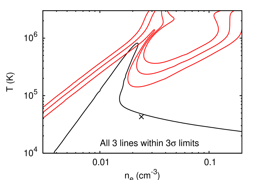
Figure 7.— Black contour: for values of ($n_{\mathrm{e}}$, $T$) below this contour there exists a time for which all three predicted line intensities simultaneously lie within the observed $3\sigma$ limits. Above this contour no such time exists. Red contours: contours showing the time $t$ after recombinations began at which the predicted O vii intensity is closest to the observed value (from bottom to top, $t=6$, 7, and $8\times 10^{5}$ yr). Black cross: This marks $n_{\mathrm{e}}=0.024$ $\mbox{cm}^{-3}$, $T=4.3\times 10^{4}$ K (Breitschwerdt, 2001; see Fig. 6).

Also for each ($n_{\mathrm{e}}$, $T$) we find the time for which the predicted O vii intensity is equal to the observed value (or closest to it, if it never actually equals it). This provides the tightest constraint on the time $t$ since recombinations began. If there are two such values (as in Figure 6) we take the later one. These results are illustrated by the red contours in Figure 7. As can be seen, the observationally acceptable region of ($n_{\mathrm{e}}$, $T$)-space (i.e. below the black contour) corresponds to $t<7\times 10^{5}$ yr, and most of this region (including the values of $n_{\mathrm{e}}$ and $T$ from Breitschwerdt 2001) corresponds to $t<6\times 10^{5}$ yr. Furthermore, the observationally acceptable region above the $6\times 10^{5}$-yr contour corresponds to $T\gtrsim 5.5\times 10^{5}$ K and $n_{\mathrm{e}}\gtrsim 0.018$ $\mbox{cm}^{-3}$. This gives a pressure $P\gtrsim 20000$ $\mbox{cm}^{-3}$ K, which is an order of magnitude larger than the pressure of the Local Cloud (Lallement, 1998). While this is not as strong a constraint as the observed oxygen line intensities, it does mean that in this region of parameter space the recombining model loses one of its main selling points.

In summary, for most of the observationally acceptable region of ($n_{\mathrm{e}}$, $T$)-space, the observed O vii intensity implies that the time since recombinations began is $t<6\times 10^{5}$ yr. We shall now show that this time is also an upper limit on the time since the Local Bubble burst out of its natal cloud, as the timescale for recombinations was shorter when the Local Bubble was smaller.

If the Local Bubble is expanding and cooling adiabatically, its temperature $T$ and volume $V$ are related by

$$TV^{\gamma-1}=\mathrm{constant},$$ (7)

where $\gamma$ is the adiabatic index ($\gamma=5/3$). Therefore, the temperature of the Local Bubble when it is of linear size $L$ is

$$T=T_{0}(L/L_{0})^{-2},$$ (8)

where $T_{0}$ and $L_{0}$ are the present-day temperature and size. Similarly, the electron density $n_{\mathrm{e}}$ is related to the present-day density ${n_{\mathrm{e}}}_{0}$ by

$$n_{\mathrm{e}}={n_{\mathrm{e}}}_{0}(L/L_{0})^{-3}.$$ (9)

The recombination timescale $t_{\mathrm{rec}}$ is defined by

$$t_{\mathrm{rec}}\equiv\frac{1}{n_{\mathrm{e}}R(T)},$$ (10)

where $R(T)$ is the recombination coefficient (see eq. [2]). This timescale may be expressed as a function of $L/L_{0}$,

$$\frac{t_{\mathrm{rec}}}{t_{\mathrm{rec,0}}}=\frac{(L/L_{0})^{3}R(T_{0})}{R(T_{0}[L/L_{0}]^{-2})},$$ (11)

where $t_{\mathrm{rec,0}}$ is the present-day recombination timescale.

Figure 8(a) shows $t_{\mathrm{rec}}/t_{\mathrm{rec,0}}$ for O vi, O vii, and O viii as functions of $L/L_{0}$, assuming a present-day temperature $T_{0}=4.3\times 10^{4}$ K (Breitschwerdt, 2001). Figure 8(b) shows the recombinations and ionization coefficients for the various process that govern the evolution of the population of O viii, again as functions of $L/L_{0}$. The ionization coefficients were calculated using data from Arnaud & Rothenflug (1985).

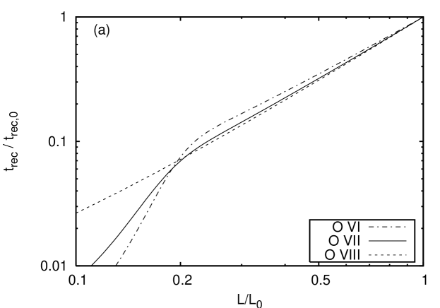
Figure 8.— (a) Recombination timescales $t_{\mathrm{rec}}$ for the formation of the labeled ions as a function of Local Bubble size $L$, assuming the Local Bubble is expanding adiabatically. The recombination timescales and $L$ have been normalized to their present-day values $t_{\mathrm{rec,0}}$ and $L_{0}$, respectively. (b) Recombination and ionization timescales for the labeled processes governing the evolution of the population of O viii. In both figures the curves were calculated assuming a present-day temperature $T_{0}=4.3\times 10^{4}$ K.

From Figure 8(a) we can see that the recombination timescale was always shorter at earlier times, when the Local Bubble was smaller. This is true for all present-day Local Bubble temperatures we investigated. From Figure 8(b), meanwhile, we can see that when $L\gtrsim 0.15L_{0}$, the recombination coefficients governing the evolution of the population of O viii are larger than the ionization coefficients (cf. in the Breitschwerdt & Schmutzler [1994] and Breitschwerdt et al. [1996] models, the Local Bubble burst out of its natal cloud when $L\approx 0.2L_{0}$). This means that since the Local Bubble burst out, recombination has dominated over ionization in the evolution of the O viii population. We find this is true in general for $T_{0}\lesssim 10^{5}$ K. This result, combined with the fact that the timescale for recombinations was shorter when the Local Bubble was younger, means that the population of O viii will be depleted more rapidly than in our original model in which $n_{\mathrm{e}}$ and $T$ are held fixed at their present-day values.

The discussion in the previous paragraph applies only to $T_{0}\lesssim 10^{5}$ K. For higher present-day temperatures ($T_{0}\sim\mbox{few}\times 10^{5}$ K), the ionization coefficients that govern the O viii evolution remain larger than the recombination coefficients for some time after the Local Bubble has burst out of its natal cloud. However, even for $T_{0}=3\times 10^{5}$ K, recombinations start to dominate the evolution of O viii before the Local Bubble reaches half its current size. Furthermore, the much lower recombination timescale at this time more than compensates for the delay in the start of recombinations – by the time the Local Bubble reaches its current size, the O viii population will be lower than if the ion populations had evolved for the same amount of time with $n_{\mathrm{e}}$ and $T$ held fixed at their present-day values.

The result of the above discussion is that the O vii emission (which in this model is formed by recombinations from O viii) will fall below the observed level on a timescale even shorter than the $\sim$$6\times 10^{5}$ yr given by our original model. Hence, as stated above, $6\times 10^{5}$ yr is an upper limit on the time since the Local Bubble burst out of its natal cloud. If the Local Bubble were any older than this, the O vii emission would be below what is observed.

This age is a factor of 2–7 times smaller than the age of the Local Bubble proposed in recombining models of the Local Bubble (Breitschwerdt & Schmutzler, 1994; Breitschwerdt et al., 1996). It also means that the Local Bubble would have expanded extremely rapidly after bursting out of its natal cloud: $(100~{}\mbox{pc})/(6\times 10^{5}~{}\mbox{yr})\approx 160$ km $\mbox{s}^{-1}$. This is much larger than the adiabatic sound speed of the ambient medium ($c_{\mathrm{s}}=15$ km $\mbox{s}^{-1}$ when $T=10^{4}$ K), and so the expansion would have been highly supersonic, resulting in a shock at the edge of the Local Bubble as it expanded, with associated heating and ionization processes. Thus, the above-described model of an adiabatically cooled, purely recombining Local Bubble is not self-consistent.

It should be noted that strictly the above argument against a recombining model of the Local Bubble only applies for present-day temperatures $T_{0}\lesssim 3\times 10^{5}$ K. However, as noted above, higher present-day temperatures which are observationally acceptable (see Fig. 7) imply a Local Bubble pressure an order of magnitude larger than that of the Local Cloud, in which case the recombining model loses one of its major selling points. It is also possible that such higher temperatures would still lead to an implausibly young Local Bubble age. However, to test this would require more detailed calculations of the growth of the Local Bubble and the ionization evolution therein, which are beyond the scope of this paper.

This is not the first time objections have been raised against a recombining model of the Local Bubble. Using values from Breitschwerdt (2001), and taking as a lower limit for the O vi fraction the value for a $5\times 10^{5}$ K plasma in equilibrium ($n_{\mathrm{O\,VI}}/n_{\mathrm{O}}=0.037$), Shelton (2003) predicted an O vi intensity of $\sim$1900 photons $\mbox{cm}^{-2}$ $\mbox{s}^{-1}$ $\mbox{sr}^{-1}$. She adds that this prediction is a lower limit, as the O vi fraction would tend to increase due to recombinations from O vii, and would not decrease again until most of the oxygen had recombined to O i and O ii. This predicted intensity is more than twice the $2\sigma$ upper limit on the Local Bubble intensity established with FUSE (Shelton, 2003). This, and a number of other discrepancies, led Shelton to conclude that recombining models could be practically eliminated.

Oegerle et al. (2005) found that a recombining model of the Local Bubble also disagrees with observations from the point of view of O vi absorption. They found that such a model leads to an O vi column density much larger than that which they had measured with FUSE.

Smith et al. (2005) considered a large set of recombining plasma models, covering a wide range of electron densities, temperatures, and Local Bubble sizes. They found that they were unable to match simultaneously the O vii and O viii intensities they measured from their Chandra spectrum of MBM 12, the upper limit on the O vi intensity (Shelton, 2003), the O vi column density (Oegerle et al., 2005), and the ROSAT R12 intensity. In essence, the R12 intensity requires a minimum density of highly ionized ions; however, the densities of O vi, O vii, and O viii are limited by the FUSE and Chandra data. Given this, Smith et al. (2005) said that a static recombining plasma model (i.e. a model in which the temperature and density governing the recombinations is constant) may be confidently disposed of.

Both Shelton’s (2003) and Smith et al.’s (2005) objections to a recombining model are based upon the predictions of a static recombining model. However, Breitschwerdt (2001) points out that for a proper recombining model of the Local Bubble, the dynamical and thermal evolution of the Local Bubble must be treated together, self-consistently. While we have not carried out full dynamical modeling of the ionization evolution in an expanding, cooling Local Bubble, we have shown that our static model gives a Local Bubble age several times smaller than that in the models of Breitschwerdt & Schmutzler (1994) and Breitschwerdt et al. (1996), and furthermore by considering the recombination timescales when the Local Bubble was smaller, we have shown that the Local Bubble age given by our static model is an upper limit on the age a dynamical model would give. To put this another way, if the Local Bubble had burst out of its natal cloud a few million years ago (Breitschwerdt & Schmutzler, 1994; Breitschwerdt et al., 1996), the O vii intensity would be far below what is observed. Our observations therefore add to the evidence against a recombining plasma model (static or dynamical) of the Local Bubble (at least with a present-day temperature $\lesssim 3\times 10^{5}$ K).

6. SUMMARY AND CONCLUSIONS

We have analyzed XMM-Newton spectra of the interstellar medium, obtained from pointings on and off an absorbing filament at high southern Galactic latitude. We have fit various models simultaneously to both sets of spectra, and used the difference in the absorbing column in the two pointing directions to constrain the spectrum of the Local Bubble.

Our main findings are as follows:

1. In the examined direction, The Local Bubble emission is consistent with emission from a thermal plasma in collisional ionization equilibrium with a temperature $\log(T_{\mathrm{LB}}/\mathrm{K})=6.06^{+0.02}_{-0.04}$ and an emission measure $\int n_{\mathrm{e}}^{2}\mathrm{d}l=0.018$ $\mbox{cm}^{-6}$ pc. The temperatures of the Local Bubble and the Galactic halo components are in good agreement with previous ROSAT measurements of other directions (Snowden et al., 1998, 2000; Kuntz & Snowden, 2000). However, our Local Bubble emission measure is 3–10 times larger than the ROSAT-determined value (Snowden et al., 1998). This discrepancy is explained by the fact that we use a different plasma emission code and abundance table from Snowden et al. (1998).

2. Our Local Bubble temperature disagrees with the results of XMM-Newton observations of the Local Bubble in other directions, which find $\log(T_{\mathrm{LB}}/\mathrm{K})\approx 6.2$ (Freyberg & Breitschwerdt, 2003; Freyberg, 2004; Freyberg et al., 2004). If we use a model with this higher $T_{\mathrm{LB}}$, we find it over-predicts the Galactic halo O vi emission by several orders of magnitude. This therefore suggests that the Local Bubble is thermally anisotropic. However, it is possible that for some of these other XMM-Newton observations the foreground emission is being contaminated by non-Local Bubble emission from Loop I.

3. Our data are also consistent with a non-equilibrium model in which the plasma is underionized. However, while an overionized recombining plasma model is observationally acceptable for certain densities and temperatures, it generally gives a very young age for the Local Bubble: $\lesssim 6\times 10^{5}$ yr. This is several times lower than the Local Bubble age in the models of Breitschwerdt & Schmutzler (1994) and Breitschwerdt et al. (1996). Such a young age is implausible, as it would require the Local Bubble to have burst highly supersonically out of its natal cloud, meaning that a purely recombining model is not self-consistent.

As stated in the Introduction, X-ray spectroscopy is essential for distinguishing between models of Local Bubble formation. The XMM-Newton observations presented here have added to the evidence against overionized, recombining models of the Local Bubble. Forthcoming Suzaku data from these same viewing directions will extend our sensitivity to lower energies, enabling us to place constraints on the carbon and nitrogen line emission in the $\sim$0.3–0.5 keV energy range. This increased spectral information will help us constrain the other major class of non-equilibrium Local Bubble model, namely an underionized plasma that is in the process of ionizing.

We would like to thank Dan McCammon, Bart Wakker, Yangsen Yao, and the referee, Joel Bregman, for helpful comments and suggestions. This work is based on observations obtained with XMM-Newton, an ESA science mission with instruments and contributions directly funded by ESA Member States and NASA. This work was funded by NASA grant NNG04GD78G (awarded through the Long Term Space Astrophysics program) and NASA grants NNG04GB68G and NNG04GB08G (awarded through the XMM-Newton Guest Investigator Program).

Appendix A MEASURING $T_{\mathrm{LB}}$ FROM FREYBERG ET AL.’S (2004) BARNARD 68 DATA

Freyberg et al. (2004) do not quote a value for $T_{\mathrm{LB}}$ measured from their XMM-Newton observation of the Bok globule Barnard 68. Here we describe how a Local Bubble temperature may be inferred from the data they do present.

Barnard 68 casts a deep shadow in the soft X-ray background. However, the shadowing is not complete at O viii energies, implying at least some of the O viii emission originates in front of Barnard 68. If one attributes this emission to the Local Bubble, then from Freyberg et al.’s (2004) Figure 2 (which gives the ratio of the on-cloud to off-cloud intensity as a function of energy) one can estimate the O vii:O viii intensity ratio for the Local Bubble emission, and hence infer a temperature.

The ratio $R_{\mathrm{O\,VIII}}$ of on-cloud to off-cloud intensity for O viii emission is

$$R_{\mathrm{O\,VIII}}=\frac{L_{\mathrm{O\,VIII}}+\mathrm{e}^{-\tau^{\mathrm{on}}_{\mathrm{O\,VIII}}}B_{\mathrm{O\,VIII}}}{L_{\mathrm{O\,VIII}}+\mathrm{e}^{-\tau^{\mathrm{off}}_{\mathrm{O\,VIII}}}B_{\mathrm{O\,VIII}}},$$ (A1)

where $L_{\mathrm{O\,VIII}}$ and $B_{\mathrm{O\,VIII}}$ are the Local Bubble and background O viii intensities, and $\tau^{\mathrm{on}}_{\mathrm{O\,VIII}}$ and $\tau^{\mathrm{off}}_{\mathrm{O\,VIII}}$ are the on- and off-cloud optical depths at O viii energies. There is a similar equation for $R_{\mathrm{O\,VII}}$, the corresponding ratio for O vii emission. The on- and off-cloud column densities are $\sim$$10^{23}$ and $\sim$$10^{20}$ $\mbox{cm}^{-2}$ (Freyberg et al., 2004). We calculate absorption cross-sections per hydrogen atom using the Bałucińska-Church & McCammon [1992] cross-sections (except for He; Yan et al., 1998) with the Wilms et al. [2000] interstellar abundances. The values at 0.57 keV (O vii) and 0.654 keV (O viii) are $6.96\times 10^{-22}$ and $4.74\times 10^{-22}$ $\mbox{cm}^{2}$, respectively. Given the large on-cloud optical depths, we can ignore the term involving $\tau^{\mathrm{on}}_{\mathrm{O\,VIII}}$ in equation (A1), and the corresponding term involving $\tau^{\mathrm{on}}_{\mathrm{O\,VII}}$ in the equation for $R_{\mathrm{O\,VII}}$. Hence, by combining equation (A1) with its $R_{\mathrm{O\,VII}}$ analogue we find that

$$\frac{L_{\mathrm{O\,VIII}}}{L_{\mathrm{O\,VII}}}=\frac{B_{\mathrm{O\,VIII}}R_{\mathrm{O\,VIII}}\mathrm{e}^{-\tau^{\mathrm{off}}_{\mathrm{O\,VIII}}}}{B_{\mathrm{O\,VII}}R_{\mathrm{O\,VII}}\mathrm{e}^{-\tau^{\mathrm{off}}_{\mathrm{O\,VII}}}}\left(\frac{1-R_{\mathrm{O\,VII}}}{1-R_{\mathrm{O\,VIII}}}\right).$$ (A2)

Figure 2 in Freyberg et al. (2004) plots the on-off intensity ratio every 50 eV. Thus, for the purposes of this estimate, we read off $R_{\mathrm{O\,VII}}$ and $R_{\mathrm{O\,VIII}}$ at 0.55 and 0.65 keV, respectively (yielding $R_{\mathrm{O\,VII}}=0.71$ and $R_{\mathrm{O\,VIII}}=0.51$), and we take the O vii and O viii “bands” to be 0.525–0.575 and 0.625–0.675 keV, respectively. If we assume the Galactic halo and extragalactic background are isotropic, we can use our “standard” model results in Table 2 to estimate that $B_{\mathrm{O\,VIII}}/B_{\mathrm{O\,VII}}=0.455$. We therefore obtain $L_{\mathrm{O\,VIII}}/L_{\mathrm{O\,VII}}=0.20$. By using XSPEC to calculate APEC model fluxes in the above energy bands, we find that this ratio corresponds to $\log(T_{\mathrm{LB}}/\mathrm{K})=6.24$ (we obtain the same value if we use MeKaL model fluxes, instead of APEC). By using a full plasma emission model to calculate flux ratios, as opposed to simply using the O vii and O viii line emissivities, we also take into account the contribution of continuum emission to the two energy bands being considered.

This estimate of $T_{\mathrm{LB}}$ assumes that the value of $B_{\mathrm{O\,VIII}}/B_{\mathrm{O\,VII}}$ measured from our XMM-Newton spectra can be applied to this pointing direction. We have also assumed a single absorption cross-section for each energy band, when in fact the absorption cross-section will vary across each band. To estimate how much of an effect these assumptions have on our result, we used a Monte Carlo method similar to that described in §5.2 to calculate 1000 values of $T_{\mathrm{LB}}$ assuming 20% errors on $B_{\mathrm{O\,VIII}}/B_{\mathrm{O\,VII}}$, $\tau^{\mathrm{on}}_{\mathrm{O\,VIII}}$, and $\tau^{\mathrm{on}}_{\mathrm{O\,VII}}$. Visual inspection of the resulting histogram of values indicates that this estimate of $T_{\mathrm{LB}}$ is accurate to within 0.1 dex (see Fig. 9).

Figure 9.— Histogram of 1000 randomly generated values of $\log(T_{\mathrm{LB}}/\mathrm{K})$, based upon the XMM-Newton observation of Barnard 68 (Freyberg et al., 2004). The temperatures were calculated from 1000 values $L_{\mathrm{O\,VIII}}/L_{\mathrm{O\,VII}}$, which in turn were calculated using equation (A2) assuming 20% errors on $B_{\mathrm{O\,VIII}}/B_{\mathrm{O\,VII}}$, $\tau^{\mathrm{on}}_{\mathrm{O\,VIII}}$, and $\tau^{\mathrm{on}}_{\mathrm{O\,VII}}$.

References

- Allen (1973) Allen, C. W. 1973, Astrophysical Quantities, 3rd edn. (London: Athlone)
- Allende Prieto et al. (2001) Allende Prieto, C., Lambert, D. L., & Asplund, M. 2001, ApJ, 556, L63
- Anders & Grevesse (1989) Anders, E., & Grevesse, N. 1989, Geochim. Cosmochim. Acta, 53, 197
- Arabadjis & Bregman (1999) Arabadjis, J. S., & Bregman, J. N. 1999, ApJ, 510, 806
- Arnaud (1996) Arnaud, K. A. 1996, in ASP Conf. Ser. 101: Astronomical Data Analysis Software and Systems V, ed. G. H. Jacoby & J. Barnes, 17
- Arnaud & Rothenflug (1985) Arnaud, M., & Rothenflug, R. 1985, A&AS, 60, 425
- Asplund et al. (2005) Asplund, M., Grevesse, N., & Sauval, A. J. 2005, in ASP Conf. Ser. 336: Cosmic Abundances as Records of Stellar Evolution and Nucleosynthesis, ed. T. G. Barnes & F. N. Bash, 25
- Asplund et al. (2004) Asplund, M., Grevesse, N., Sauval, A. J., Allende Prieto, C., & Kiselman, D. 2004, A&A, 417, 751
- Bałucińska-Church & McCammon (1992) Bałucińska-Church, M., & McCammon, D. 1992, ApJ, 400, 699
- Bevington & Robinson (2003) Bevington, P. R., & Robinson, D. K. 2003, Data Reduction and Error Analysis for the Physical Sciences, 3rd edn. (New York: McGraw-Hill)
- Bowyer et al. (1968) Bowyer, C. S., Field, G. B., & Mack, J. E. 1968, Nature, 217, 32
- Breitschwerdt (1996) Breitschwerdt, D. 1996, SSRv, 78, 173
- Breitschwerdt (1998) Breitschwerdt, D. 1998, in Lecture Notes in Physics 506, The Local Bubble and Beyond, ed. D. Breitschwerdt, M. J. Freyberg, & J. Trümper (New York: Springer), 5
- Breitschwerdt (2001) —. 2001, Ap&SS, 276, 163
- Breitschwerdt & Cox (2004) Breitschwerdt, D., & Cox, D. P. 2004, in How Does the Galaxy Work? A Galactic Tertulia with Don Cox and Ron Reynolds, ed. E. J. Alfaro, E. Pérez, & J. Franco (Dordrecht: Kluwer), 391
- Breitschwerdt & de Avillez (2006) Breitschwerdt, D., & de Avillez, M. A. 2006, A&A, 452, L1
- Breitschwerdt et al. (1996) Breitschwerdt, D., Egger, R., Freyberg, M. J., Frisch, P. C., & Vallerga, J. V. 1996, SSRv, 78, 183
- Breitschwerdt & Schmutzler (1994) Breitschwerdt, D., & Schmutzler, T. 1994, Nature, 371, 774
- Burrows & Mendenhall (1991) Burrows, D. N., & Mendenhall, J. A. 1991, Nature, 351, 629
- Chen et al. (1997) Chen, L.-W., Fabian, A. C., & Gendreau, K. C. 1997, MNRAS, 285, 449
- Cox (1998) Cox, D. P. 1998, in Lecture Notes in Physics 506, The Local Bubble and Beyond, ed. D. Breitschwerdt, M. J. Freyberg, & J. Trümper (New York: Springer), 122
- Cox & Anderson (1982) Cox, D. P., & Anderson, P. R. 1982, ApJ, 253, 268
- Diplas & Savage (1994) Diplas, A., & Savage, B. D. 1994, ApJ, 427, 274
- Freyberg (2004) Freyberg, M. J. 2004, Ap&SS, 289, 229
- Freyberg & Breitschwerdt (2003) Freyberg, M. J., & Breitschwerdt, D. 2003, AN, 324, 162
- Freyberg et al. (2004) Freyberg, M. J., Breitschwerdt, D., & Alves, J. 2004, Mem. Soc. Astron. It., 75, 509
- Grevesse & Sauval (1998) Grevesse, N., & Sauval, A. J. 1998, SSRv, 85, 161
- Innes & Hartquist (1984) Innes, D. E., & Hartquist, T. W. 1984, MNRAS, 209, 7
- Jelinksy et al. (1995) Jelinksy, P., Vallerga, J. V., & Edelstein, J. 1995, ApJ, 442, 653
- Juda et al. (1991) Juda, M., Bloch, J. J., Edwards, B. C., McCammon, D., Sanders, W. T., Snowden, S. L., & Zhang, J. 1991, ApJ, 367, 182
- Kuntz & Snowden (2000) Kuntz, K. D., & Snowden, S. L. 2000, ApJ, 543, 195
- Kuntz et al. (1997) Kuntz, K. D., Snowden, S. L., & Verter, F. 1997, ApJ, 484, 245
- Lallement (1998) Lallement, R. 1998, in Lecture Notes in Physics 506, The Local Bubble and Beyond, ed. D. Breitschwerdt, M. J. Freyberg, & J. Trümper (New York: Springer), 19
- Lallement et al. (2003) Lallement, R., Welsh, B. Y., Vergely, J. L., Crifo, F., & Sfeir, D. 2003, A&A, 411, 447
- Maíz-Apellániz (2001) Maíz-Apellániz, J. 2001, ApJ, 560, L83
- Masai (1994) Masai, K. 1994, ApJ, 437, 770
- Mazzotta et al. (1998) Mazzotta, P., Mazzitelli, G., Colafrancesco, S., & Vittorio, N. 1998, A&AS, 133, 403
- McCammon et al. (2002) McCammon, D., Almy, R., Apodaca, E., Bergmann Tiest, W., Cui, W., Deiker, S., Galeazzi, M., Juda, M., Lesser, A., Mihara, T., Morgenthaler, J. P., Sanders, W. T., Zhang, J., Figueroa-Feliciano, E., Kelley, R. L., Moseley, S. H., Mushotzky, R. F., Porter, F. S., Stahle, C. K., & Szymkowiak, A. E. 2002, ApJ, 576, 188
- Mewe & Gronenschild (1981) Mewe, R., & Gronenschild, E. H. B. M. 1981, A&AS, 45, 11
- Mewe et al. (1985) Mewe, R., Gronenschild, E. H. B. M., & van den Oord, G. H. J. 1985, A&AS, 62, 197
- Mewe et al. (1995) Mewe, R., Kaastra, J. S., & Liedahl, D. A. 1995, Legacy, 6, 16
- Oegerle et al. (2005) Oegerle, W. R., Jenkins, E. B., Shelton, R. L., Bowen, D. V., & Chayer, P. 2005, ApJ, 622, 377
- Penprase et al. (1998) Penprase, B. E., Lauer, J., Aufrecht, J., & Welsh, B. Y. 1998, ApJ, 492, 617
- Protassov et al. (2002) Protassov, R., van Dyk, D. A., Connors, A., Kashyap, V. L., & Siemiginowska. 2002, ApJ, 571, 545
- Raymond (1991) Raymond, J. C. 1991, Update to Raymond & Smith (1977) code, ftp://heasarc.gsfc.nasa.gov/software/plasma_codes/raymond/
- Raymond & Smith (1977) Raymond, J. C., & Smith, B. W. 1977, ApJS, 35, 419
- Reynolds (1990) Reynolds, R. J. 1990, ApJ, 348, 153
- Reynolds (1991) Reynolds, R. J. 1991, in Proc. IAU Symp. 144, The Interstellar Disk-Halo Connection in Galaxies, ed. H. Bloemen, 67
- Sanders et al. (1977) Sanders, W. T., Kraushaar, W. L., Nousek, J. A., & Fried, P. M. 1977, ApJ, 217, L87
- Schlegel et al. (1998) Schlegel, D. J., Finkbeiner, D. P., & Davis, M. 1998, ApJ, 500, 525
- Sfeir et al. (1999) Sfeir, D. M., Lallement, R., Crifo, F., & Welsh, B. Y. 1999, A&A, 346, 785
- Shelton (2003) Shelton, R. L. 2003, ApJ, 589, 261
- Shull & Slavin (1994) Shull, J. M., & Slavin, J. D. 1994, ApJ, 427, 784
- Shull & van Steenberg (1982) Shull, J. M., & van Steenberg, M. 1982, ApJS, 48, 95
- Smith et al. (2001) Smith, R. K., Brickhouse, N. S., Liedahl, D. A., & Raymond, J. C. 2001, ApJ, 556, L91
- Smith & Cox (2001) Smith, R. K., & Cox, D. P. 2001, ApJS, 134, 283
- Smith et al. (2005) Smith, R. K., Edgar, R. J., Plucinsky, P. P., Wargelin, B. J., Freeman, P. E., & Biller, B. A. 2005, ApJ, 623, 225
- Snowden et al. (2004) Snowden, S. L., Collier, M. R., & Kuntz, K. D. 2004, ApJ, 610, 1182
- Snowden et al. (1998) Snowden, S. L., Egger, R., Finkbeiner, D. P., Freyberg, M. J., & Plucinsky, P. P. 1998, ApJ, 493, 715
- Snowden et al. (1997) Snowden, S. L., Egger, R., Freyberg, M. J., McCammon, D., Plucinsky, P. P., Sanders, W. T., Schmitt, J. H. M. M., Trümper, J., & Voges, W. 1997, ApJ, 485, 125
- Snowden et al. (2000) Snowden, S. L., Freyberg, M. J., Kuntz, K. D., & Sanders, W. T. 2000, ApJS, 128, 171
- Snowden et al. (1994) Snowden, S. L., Hasinger, G., Jahoda, K., Lockman, F. J., McCammon, D., & Sanders, W. T. 1994, ApJ, 430, 601
- Snowden et al. (1993) Snowden, S. L., McCammon, D., & Verter, F. 1993, ApJ, 409, L21
- Snowden et al. (1991) Snowden, S. L., Mebold, U., Hirth, W., Herbstmeier, U., & Schmitt, J. H. M. M. 1991, Science, 252, 1529
- Tanaka & Bleeker (1977) Tanaka, Y., & Bleeker, J. A. M. 1977, SSRv, 20, 815
- Vallerga & Slavin (1998) Vallerga, J., & Slavin, J. 1998, in Lecture Notes in Physics 506, The Local Bubble and Beyond, ed. D. Breitschwerdt, M. J. Freyberg, & J. Trümper (New York: Springer), 79
- Verner & Ferland (1996) Verner, D. A., & Ferland, G. J. 1996, ApJS, 103, 467
- Wilms et al. (2000) Wilms, J., Allen, A., & McCray, R. 2000, ApJ, 542, 914
- Yan et al. (1998) Yan, M., Sadeghpour, H. R., & Dalgarno, A. 1998, ApJ, 496, 1044