Internal dynamics of the radio halo cluster Abell 773:
a multiwavelength analysis

Abstract

Aims. To conduct an intensive study of the rich, X-ray luminous galaxy cluster Abell 773 at $z=0.22$ containing a diffuse radio halo to determine its dynamical status.

Methods. Our analysis is based on new spectroscopic data obtained at the TNG telescope for 107 galaxies, 37 spectra recovered from the CFHT archive and new photometric data obtained at the Isaac Newton Telescope. We use statistical tools to select 100 cluster members (out to $\sim$1.8 $h_{70}^{-1}$ Mpc from the cluster centre), to analyse the kinematics of cluster galaxies and to determine the cluster structure. Our analysis is also performed by using X-ray data stored in the Chandra archive.

Results. The 2D distribution shows two significant peaks separated by $\sim$2$\mathrm{{}^{\prime}}\;$in the EW direction with the main western one closely located at the position of the two dominant galaxies and the X-ray peak. The velocity distribution of cluster galaxies shows two peaks at ${\rm v}\sim$65000 and $\sim$67500 km s^-1, corresponding to the velocities of the two dominant galaxies. The low velocity structure has a high velocity dispersion – $\sigma_{\rm v}=800-1100$ km s${}^{-1}\;$– and its galaxies are centred on the western 2D peak. The high velocity structure has intermediate velocity dispersion – $\sigma_{\rm v}\sim 500$ km s${}^{-1}\;$– and is characterized by a complex 2D structure with a component centred on the western 2D peak and a component centred on the eastern 2D peak, these components probably being two independent groups. We estimate a cluster mass within 1 $h_{70}^{-1}$ Mpc of 6–11 $\times 10^{14}\;h_{70}^{-1}\;M_{\odot}$. Our analysis of Chandra data shows the presence of two very close peaks in the core and the elongation of the X-ray emission in the NEE–SWW direction.

Conclusions. Our results suggest we are looking at probably two groups in an advanced stage of merging with a main cluster and having an impact velocity $\Delta{{\rm v}_{\rm rf}}\sim 2300$ km s^-1. In particular, the radio halo seems to be related to the merger of the eastern group.

1 Introduction

Clusters of galaxies are recognized to be not simple relaxed structures, but rather as evolving via merging processes in a hierarchical fashion from poor groups to rich clusters. Much progress has been made in recent years in the observations of the signatures of merging processes (see Feretti et al. fer02b (2002) for a general review). The presence of substructure, which is indicative of a cluster at an early phase of the process of dynamical relaxation or of secondary infall of clumps into already virialized clusters occurs in about 50% of clusters as shown by optical and X-ray data (e.g. Geller & Beers gel82 (1982); Mohr et al. moh96 (1996); Girardi et al. gir97 (1997); Kriessler & Beers kri97 (1997); Jones & Forman jon99 (1999); Schuecker et al. sch01 (2001); Burgett et al. bur04 (2004)).

A very interesting aspect of these investigations is the possible connection of cluster mergers with the presence of extended diffuse radio sources, halos and relics. They are rare, large (up to $\sim 1$–2 $h_{70}^{-1}$ Mpc), amorphous cluster sources of uncertain origin and generally steep radio spectra (Hanisch han82 (1982); see also Giovannini & Feretti gio02 (2002) for a recent review). They appear to be associated with very rich clusters that have undergone recent mergers, and it has therefore been suggested by various authors that cluster halos/relics are related to recent merger activity (e.g. Tribble tri93 (1993); Burns et al. bur94 (1994); Feretti fer99 (1999)).

The synchrotron radio emission of halos and relics demonstrates the existence of large scale cluster magnetic fields, of the order of 0.1–1 $\mu$G, and of widespread relativistic particles of energy density 10^-14 – 10^-13 erg cm^-3. The difficulty in explaining radio halos arises from the combination of their large size and the short synchrotron lifetime of relativistic electrons. The expected diffusion velocity of the electron population is of the order of the Alfven speed ($\sim$100 km s^-1) making it difficult for the electrons to diffuse over a megaparsec-scale region within their radiative lifetime. Therefore, one needs a mechanism by which the relativistic electron population can be transported over large distances in a short time, or a mechanism by which the local electron population is reaccelerated and the local magnetic fields are amplified over an extended region. The cluster–cluster merger can potentially supply both mechanisms (e.g. Giovannini et al. gio93 (1993); Burns et al. bur94 (1994); Röttgering et al. rot94 (1994); see also Feretti et al. fer02a (2002); Sarazin sar02 (2002) for reviews). However, the question is still debated since the diffuse radio sources are quite uncommon and only recently we have been able to study these phenomena on the basis of sufficient statistics (a few dozen clusters up to $z\sim 0.3$, e.g. Giovannini et al. gio99 (1999); see also Giovannini & Feretti gio02 (2002); Feretti fer05 (2005)).

Growing evidence for the connection between diffuse radio emission and cluster merging is based on X-ray data (e.g. Böhringer & Schuecker boh02 (2002); Buote buo02 (2002)). Studies based on a large number of clusters have found a significant relation between the radio and the X-ray surface brightness (Govoni et al. 2001a , 2001b ) and between the presence of radio halos/relics and irregular and bimodal X-ray surface brightness distribution (Schuecker et al. sch01 (2001)). New unprecedent insights into merging processes in radio clusters are offered by Chandra and XMM–Newton observations (e.g. Markevitch & Vikhlinin mar01 (2001); Markevitch et al. mar02 (2002); Fujita et al. fuj04 (2004); Henry et al. hen04 (2004); Kempner & David kem04 (2004)).

Optical data are a powerful way to investigate the presence and the dynamics of cluster mergers, too (e.g. Girardi & Biviano gir02 (2002)). The spatial and kinematic analysis of member galaxies allow us to detect and measure the amount of substructure, to identify and analyse possible pre-merging clumps or merger remnants. This optical information is complementary to X-ray information since galaxies and ICM react on different time scales during a merger (see, for example, numerical simulations by Roettiger et al. roe97 (1997)). Unfortunately, to date optical data are lacking or are poorly exploited. The sparse literature contains a few individual clusters (e.g. Colless & Dunn col96 (1996); Gómez et al. gom00 (2000); Barrena et al. bar02 (2002); Mercurio et al. mer03 (2003); Boschin et al. bos04 (2004); Boschin et al. bos06 (2006); Girardi et al. gir06 (2006)). We have conducted an intensive study of Abell 773 (hereafter A773), which has a radio halo (Giovannini et al. gio99 (1999), see also Kempner & Sarazin kem01 (2001)).

A773 is a rich, X-ray luminous and hot cluster at $z\sim 0.22$: Abell richness class = 2 (Abell et al. abe89 (1989)), $L_{\mathrm{X}}$(0.1–2.4 keV)$=12.52\times 10^{44}\ h_{50}^{-2}$ erg s^-1 (Ebeling et al. ebe96 (1996)), $T_{\mathrm{X}}\sim 7$–9 keV (Allen & Fabian all98 (1998); Rizza et al. riz98 (1998); White whi00 (2000); Saunders et al. sau03 (2003); Govoni et al. gov04 (2004); Ota & Mitsuda ota04 (2004)). This cluster has a centre that is extremely optically rich and contains almost only early-type galaxies (Dahle et al. dah02 (2002)). A lot of evidence points towards the young dynamical status of A773. This cluster is elongated along the NE–SW direction and has a great amount of substructure in X-ray emission, as shown by ROSAT HRI data (Pierre & Starck pie98 (1998); Rizza et al. riz98 (1998); Govoni et al. 2001b ). There is a strong peak in the mass map, offset to the southwest from the optical centre by about 1$\mathrm{{}^{\prime}}\;$and the mass appears to be elongated in a different way with respect to the light and number density distribution (Dahle et al. dah02 (2002)). The optical DSS image clearly shows two galaxy substructures, one in the centre of the X-ray emission and another at the eastern region (Govoni et al. gov04 (2004)).

To date, few spectroscopic data have been reported in the literature. Crawford et al. (cra95 (1995)) measured the redshift for the two brightest, equally dominant galaxies ($z\sim 0.22$). A few redshifts for radio galaxies in the cluster region are given by Morrison et al. (mor03 (2003)). We have recently carried out spectroscopic observations with the TNG giving new redshift data for 107 galaxies in the field of A773, as well as photometric observations at the INT. We recover additional spectroscopic information from reduction of CFHT archive data. Our present analysis is based on these optical data and X-ray Chandra archival data.

This paper is organized as follows. We present the new optical data in Sect. 2 and the relevant analyses in Sect. 3. Our analysis of Chandra X-ray data is shown in Section 4. We discuss the dynamical status of A773 in Sect. 5 and summarize our results in Section 6.

Unless otherwise stated, we give errors at the 68% confidence level (hereafter c.l.). Throughout the paper, we assume a flat cosmology with $\Omega_{\rm m}=0.3$, $\Omega_{\Lambda}=0.7$ and $H_{0}=70$ $h_{70}$ km s${}^{-1}\;$Mpc^-1. For this cosmological model, 1$\mathrm{{}^{\prime}}\;$corresponds to 213 $h_{70}^{-1}$ kpc at the cluster redshift.

2 Data sample

2.1 Spectroscopy

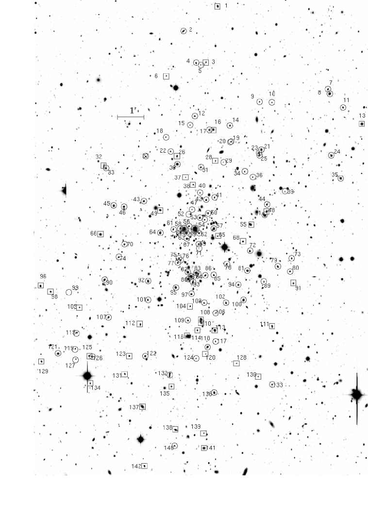
Figure 1: $R$-band image of A773 (west at the top and north to the left) taken with the WFC camera of the INT. Galaxies with successful velocity measurements are labelled as in Table 3. Circles and boxes indicate cluster members and non-member galaxies, respectively.

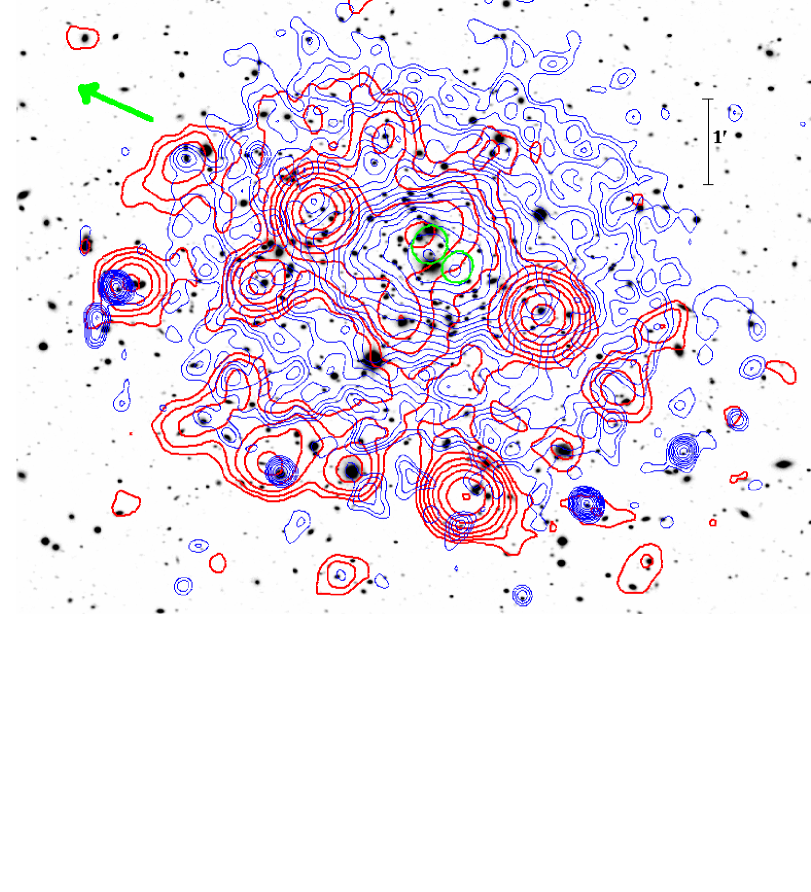
Figure 2: $R$-band image of the cluster A773 with, superimposed, the contour levels of the Chandra archival image ID 5006 (blue; photons in the energy range 0.3–7 keV) and the contour levels of a VLA radio image (red) at 1.4 GHz (Govoni et al. 2001b ). Green ellipses identify structures detected by Wavdetect. The direction of A782 is also shown (see Sect. 5.4). North is at the top and east to the left.

Multi-object spectroscopic observations of A773 were carried out at the TNG in December 2003 during the programme of proposal AOT8/CAT–G6. We used DOLORES/MOS with the LR–B Grism 1, giving a dispersion of 187 Å/mm, and the Loral $2048\times 2048$ CCD (pixel size 15 $\mu$m). This combination of grating and detector results in a dispersion of 2.8 Å/pix. We have taken four MOS masks for a total of 137 slits. We acquired two exposures of 1800 s for one mask and three exposures of 1800 s for three masks. Wavelength calibration was performed using helium–argon lamps.

Reduction of spectroscopic data was carried out with the IRAF package.

Radial velocities were determined using the cross-correlation technique (Tonry & Davis ton79 (1979)) implemented in the RVSAO package (developed at the Smithsonian Astrophysical Observatory Telescope Data Center). Each spectrum was correlated against six templates for a variety of galaxy spectral types: E, S0, Sa, Sb, Sc and Ir (Kennicutt ken92 (1992)). The template producing the highest value of $\cal R$, i.e. the parameter given by RVSAO and related to the signal-to-noise of the correlation peak, was chosen. Moreover, all the spectra and their best correlation functions were examined visually to verify the redshift determination. In two cases (IDs 66 and 129; see Table 3) we took the EMSAO redshift as a reliable estimate of the redshift. We obtained redshifts for 107 galaxies.

For six galaxies we obtained two redshift determinations of similar quality. This allows us to obtain a more rigorous estimate for the redshift errors since the nominal errors as given by the cross-correlation are known to be smaller than the true errors (e.g. Malumuth et al. mal92 (1992); Bardelli et al. bar94 (1994); Ellingson & Yee ell94 (1994); Quintana et al. qui00 (2000)). For the six galaxies having two redshift determinations we fit the first determination vs. the second one by using a straight line and considering errors in both coordinates (e.g. Press et al. pre92 (1992)). The fitted line agrees with the one-to-one relation, but, when using the nominal cross-correlation errors, the small value of $\chi^{2}$ probability indicates a poor fit, suggesting the errors are underestimated. Only when nominal errors are multiplied by a factor of $\sim$1.5 can the observed scatter be justified. We therefore assume hereafter that true errors are larger than nominal cross-correlation errors by a factor 1.5. For the six galaxies we used the average of the two redshift determinations and the corresponding error.

We added to our data observations stored in the CFHT archive (proposal ID: 01AF37): 1 MOS mask of three 1800 s exposures with 52 slits. We reduced the spectra with the same procedure adopted for the TNG observations. We succeeded in obtaining spectra for 37 galaxies, two of which are in common with TNG galaxies. The comparison of the two estimates agree well within the errors ($cz_{\rm CFHT}=44170\pm 199$ vs. $cz_{\rm TNG}=44195\pm 94$ km s^-1, $cz_{\rm CFHT}=64304\pm 113$ vs. $cz_{\rm TNG}=64260\pm 46$ km s^-1), allowing us to combine the data. For the two galaxies in common we used the average of the two redshift determinations and the corresponding error.

Our spectroscopic catalogue consists of 142 galaxies in a region of 18^′$\times$13$\mathrm{{}^{\prime}}\;$centred on the position of the two close dominant galaxies (IDs 59 and 60, hereafter D1 and D2; see Table 3). The median $S/N$ and error on $cz$ are 12 and 72 km s^-1, respectively.

We use a conservative approach leading to a sparse spectral classification (75% of the sample, see Table 3). We follow the classification of Dressler et al. (dre99 (1999); see also Poggianti et al. pog99 (1999)). We define “e”-type galaxies as those showing active star formation indicated by the presence of [OII], and, in particular, “e(b)” galaxies as those showing an equivalent width EW([OII]) of $\leq-40$ Å   (probably starburst galaxies). Of galaxies having $S/N\mathrel{\hbox{\hbox to0.0pt{\hbox{\lower 4.0pt\hbox{$\sim$}}\hss}\hbox{$>$}}}10\,\,$ we define as “k”-type those having EW(H$\delta$)$<$3 Å  and no emission lines (probably passive galaxies); “k+a”- and “a+k”-type galaxies as those having $3\leq$EW(H$\delta$)$\leq$8 Å  and EW(H$\delta$)$>$8 Å, respectively, and no emission lines (the “post-starbust” galaxies of Couch et al. cou94 (1994)); “e(a)”-type galaxies as those having emission lines and EW(H$\delta$)$\geq$4 Å ; “e(c)”-type galaxies as those having emission lines and EW(H$\delta$)$<$4 Å  (probably spiral galaxies). Galaxy ID 89, which is the only one showing any emission lines ([OIII] in this case), but having the [OII] line outside the observed spectral range, is classified as “e(a)”. Out of 106 classified galaxies (94 with $S/N\mathrel{\hbox{\hbox to0.0pt{\hbox{\lower 4.0pt\hbox{$\sim$}}\hss}\hbox{$>$}}}10$) we find 68 “passive” galaxies and 38 “active” galaxies (starbust and poststarbust; i.e. 6:1:8:9:5:9 for k+a:a+k:e(c):e(a):e(b):e, respectively). Of nine galaxies of type “e”, i.e. those moderate emission line galaxies with low $S/N$, six are probably of type e(c) and three are probably of type e(a) (hereafter e(c?) and e(a?)).

2.2 Photometry

Our photometric observations were carried out with the Wide Field Camera (WFC), mounted at the prime focus of the 2.5 m INT (located at Roque de los Muchachos Observatory, La Palma, Spain). We observed A773 in December 2004 in photometric conditions with a seeing of about 1.4$\mathrm{{}^{\prime}}\hskip-1.00006pt\mathrm{{}^{\prime}}\;$.

The WFC consists of a four-CCD mosaic covering a 33^′$\times$33$\mathrm{{}^{\prime}}\;$field of view, with only a 20% marginally vignetted area. We took nine exposures of 720 s in $B_{\rm H}$ and 300 s in $R_{\rm H}$ Harris filters (a total of 6480 s and 2700 s in each band) developing a dithering pattern of nine positions. This observing mode allowed us to build a “supersky” frame that was used to correct our images for fringing patterns (Gullixson gul92 (1992)). In addition, the dithering helped us to clean cosmic rays and avoid gaps between the CCDs in the final images. The complete reduction process (including flat fielding, bias subtraction and bad-column elimination) yielded a final coadded image where the variation of the sky was lower than 0.4% in the whole frame. Another effect associated with the wide field frames is the distortion of the field. In order to match the photometry of several filters, a good astrometric solution is needed to take into account these distortions. Using IRAF tasks and taking as a reference the USNO B1.0 catalogue, we were able to find an accurate astrometric solution (rms $\sim$ 0.5$\mathrm{{}^{\prime}}\hskip-1.00006pt\mathrm{{}^{\prime}}$) across the full frame. The photometric calibration was performed using Landolt standard fields obtained during the observation.

We finally identified galaxies in our $B_{\rm H}$ and $R_{\rm H}$ images and measured their magnitudes with the SExtractor package (Bertin & Arnouts ber96 (1996)) and AUTOMAG procedure. In a few cases (e.g. close companion galaxies, galaxies close to defects of the CCD) the standard SExtractor photometric procedure failed. In these cases we computed magnitudes by hand. This method consists in assuming a galaxy profile of a typical elliptical and scaling it to the maximum observed value. The integration of this profile gives us an estimate of the magnitude. This method is similar to PSF photometry, but assumes a galaxy profile, more appropriate in this case.

We transformed all magnitudes into the Johnson–Cousins system (Johnson & Morgan joh53 (1953); Cousins cou76 (1976)). We used $B=B\rm_{H}+0.13$ and $R=R\rm_{H}$ as derived from the Harris filter characterization (http://www.ast.cam.ac.uk/$\sim$wfcsur/technical/photom/colours/) and assuming a $B-V\sim 1.0$ for E-type galaxies (Poggianti pog97 (1997)). As a final step, we estimated and corrected the galactic extinction $A_{B}\sim 0.06$, $A_{R}\sim 0.04$ from Burstein & Heiles’s (bur82 (1982)) reddening maps.

We estimated that our photometric sample is complete down to $R=22.4$ (23.6) and $B=20.4$ (22.5) for $S/N=5$ (3) within the observed field.

We assigned magnitudes to 141 of the 142 galaxies of our spectroscopic catalogue. We measured redshifts for galaxies down to magnitude $R\sim$ 21, but a high level of completeness is reached only for galaxies with magnitude $R<$ 19.5 ($\sim$50% completeness).

Table 3 (available in electronic format) lists the velocity catalogue (see also Fig. 1 and Fig. 2): identification number ID (Col. 1), identification label of each galaxy following IAU nomenclature rules (Col. 2); right ascension and declination, $\alpha$ and $\delta$ (J2000, Col. 3); $B$ magnitudes (Col. 4); $R$ magnitudes (Col. 5); heliocentric radial velocities, ${\rm v}=cz_{\sun}$ (Col. 6) with errors, $\Delta{\rm v}$ (Col. 7); spectral classification (Col. 8).

3 Analysis of optical data

3.1 Member selection and global properties

To select cluster members from 142 galaxies having redshifts, we use the adaptive-kernel method (hereafter DEDICA, Pisani pis93 (1993) and pis96 (1996); see also Fadda et al. fad96 (1996); Girardi et al. gir96 (1996); Girardi & Mezzetti gir01 (2001)). We find significant peaks in the velocity distribution $>$99% c.l.. This procedure detects A773 as a two-peaked structure, populated by 100 galaxies with $62250<{\rm v}<68850$ km s^-1, hereafter referred as cluster members (see Table 3 and Fig. 3). Of the non-member galaxies, 24 and 18 are foreground and background galaxies, respectively. In particular, 15 foreground galaxies belong to a low density peak at $z\sim 0.186$.

Figure 3: Redshift galaxy distribution. The solid line histogram refers to galaxies assigned to the cluster according to the DEDICA reconstruction method.

By applying the biweight estimator to cluster members (Beers et al. bee90 (1990)), we compute a mean cluster redshift of $\left<z\right>=0.2197\pm$ 0.0005, i.e. $\left<\rm{\rm v}\right>=65876\pm$140 km s^-1. We estimate the LOS velocity dispersion, $\sigma_{\rm v}$, by using the biweight estimator and applying the cosmological correction and the standard correction for velocity errors (Danese et al. dan80 (1980)). We obtain $\sigma_{\rm v}=1394_{-68}^{+84}$ km s^-1, where errors are estimated through a bootstrap technique.

Hereafter, we consider as cluster centre the position of the most luminous dominant galaxy [D1, R.A.=$09^{\mathrm{h}}17^{\mathrm{m}}53\,\hbox to0.0pt{\hbox{$\mathrm{{}^{s}}$}\hss}{\hbox{$.$}}\,26$, Dec.=$+51\mathrm{{}^{\circ}}43\mathrm{{}^{\prime}}36\,\hbox to0.0pt{\hbox{$\mathrm{{}^{\prime}\hskip-1.00006pt{}^{\prime}}$}\hss}{\hbox{$.$}}\,5$ (J2000.0)], which is related to the richer subsystem as shown in the following sections.

3.2 Bimodal velocity structure

The DEDICA method assigns 63 galaxies with ${\rm v}\leq 66543$ km s${}^{-1}\;$to a peak at $cz=65013$ km s${}^{-1}\;$and 37 galaxies with ${\rm v}\geq 66653$ km s${}^{-1}\;$at a peak at $cz=67453$ ($z\sim 0.217$ and $z\sim 0.224$, respectively, see Figure 4). According to the working definition of Girardi et al. (gir96 (1996)), the two peaks are not easily separable since their overlap is very large, i.e. many galaxies (63/100) have a non-negligible probability of belonging to both peaks.

Figure 4: Lower panel: rest-frame velocity vs. projected distance from the cluster centre – the location of the dominant galaxy D1 – of the 100 galaxies assigned to the cluster (Fig. 3). Upper panel: velocity histogram of the 100 galaxies assigned to the cluster. Velocities of the two dominant galaxies are pointed out. The two–peaks detected by the DEDICA method and the two Gaussians corresponding to the KMM partition (see Table 2) are also shown (faint and dashed lines, respectively).

The DEDICA method used above has the advantage of not requiring any a priori shape for the subsystem research. Kaye’s Mixture Model (KMM, as implemented by Ashman et al. ash94 (1994)), which fits a user-specified number of Gaussian distributions, gives a quite similar result. Of the cluster members we find that the KMM method fits a two-group partition by rejecting the single Gaussian at the 99.7% c.l., as obtained from the likelihood ratio test, assigning the 65 galaxies with ${\rm v}\leq 66659$ km s${}^{-1}\;$and the 35 galaxies ${\rm v}\geq 66845$ km s${}^{-1}\;$to two different groups.

Finally, we note that the two dominant galaxies of the cluster are assigned to different groups: D1 lies very close to the low velocity peak and D2 lies very close to the peak of the high velocity peak (Fig. 4).

We present the main properties for low- and high-velocity structures as defined by both the DEDICA method (hereafter LV- and HV-groups, respectively) and the KMM method (hereafter, KMM1 and KMM2, respectively). Table 2 lists the name of the sample (Col. 1); the number of assigned members, $N_{\rm g}$ (Col. 2); the mean velocity and its error, $<{\rm v}>$ (Col. 3); the velocity dispersion and its bootstrap errors, $\sigma_{\rm v}$ (Col. 4). The above properties are computed using the galaxies assigned to each individual group. However, since there is a wide velocity range where galaxies have a non-zero probability of belonging to both groups, both DEDICA and KMM group membership assignment leads to an artificial truncation of the distributions being “deconvolved” (see the velocity thresholds above). This truncation may lead to an underestimate of velocity dispersion for the subclusters (see Bird bir94 (1994)). Therefore, we also list the value of $\sigma_{\rm v}$ as computed by KMM software using the galaxies of the whole sample weighted with their assignment probabilities to the respective sample after having applied the cosmological correction and the standard correction for velocity errors (Danese et al. dan80 (1980)).

Table 2: Results of the kinematical analysis

$$\begin{array}[]{l r l l}\hline\cr\vskip 3.0pt plus 1.0pt minus 1.0pt\cr\hline\cr\vskip 3.0pt plus 1.0pt minus 1.0pt\cr\mathrm{Sample}&\mathrm{N_{g}}&\phantom{249}<{\rm v}>^{\mathrm{a}}\phantom{249}&\phantom{24}\sigma_{\rm v}^{\mathrm{b}}\phantom{24}\\ &&\phantom{249}\mathrm{km\ s^{-1}}\phantom{249}&\phantom{2}\mathrm{km\ s^{-1}}\phantom{24}\\ \hline\cr\vskip 3.0pt plus 1.0pt minus 1.0pt\cr\mathrm{Whole\ system}&100&65876\pm 140&1394_{-68}^{+84}\\ \mathrm{LV-group}&63&64875\pm 105&825_{-63}^{+102}\\ \mathrm{HV-group}&37&67664\pm 86&515_{-43}^{+53}\\ \mathrm{KMM1}&65&64924\pm 107&858_{-73}^{+96}(1122)^{\mathrm{c}}\\ \mathrm{KMM2}&35&67717\pm 83&484_{-40}^{+50}(548)^{\mathrm{c}}\\ \mathrm{W-sub}&14&65573\pm 366&1299_{-118}^{+220}\\ \mathrm{E-sub}&5&67469\pm 86&473_{-25}^{+286}\\ \mathrm{LV-W-sub}&8&64415\pm 198&493_{-43}^{+107}\\ \mathrm{HV-W-sub}&6&67187\pm 262&539_{-50}^{+84}\\ \mathrm{LV-very\ red}&28&64962\pm 100&518_{-64}^{+76}\\ \mathrm{HV-very\ red}&15&67579\pm 138&506_{-97}^{+149}\\ \vskip 3.0pt plus 1.0pt minus 1.0pt\cr\hline\cr\vskip 3.0pt plus 1.0pt minus 1.0pt\cr\hline\cr\end{array}$$

• For comparison $\rm v$ of D1 and D2 dominant galaxies are 65131 and 67765 km  s^-1.

• We use the biweight and the gapper estimators by Beers et al. (bee90 (1990)) for samples with $\mathrm{N_{g}}\geq$ 15 and with $\mathrm{N_{g}}<15$ galaxies, respectively (see also Girardi et al. gir93 (1993)).

• Between parenthesis we list (standard) velocity dispersions as computed by using the galaxies of the whole system weighted with their assignment probabilities to the respective sample rather then only the galaxies assigned to the samples (see text).

Since the velocity difference between the two groups is probably of a dynamical nature (see Sect. 5) we expect that the magnitude incompleteness of our sample affects both in a similar way, thus having a small influence on their detection and kinematic properties. To verify this issue, of 142 galaxies having redshifts we select samples of 98 (62) galaxies brighter than 19.5 (19) mags for which the completeness is at least $\sim 50$%. In both cases the KMM method detects the two peaks at similar mean velocities. The estimates of velocity dispersions agree within 1–1.5 sigma with the values obtained in the whole sample (i.e. $\sigma_{\rm v}=750_{-85}^{+146}$, $671_{-50}^{+110}$ km s${}^{-1}\;$and $\sigma_{\rm v}=514_{-68}^{+82}$, $474_{-118}^{+126}$ km s${}^{-1}\;$for the main and secondary peaks, respectively – to be compared with KMM1 and KMM2 values).

3.3 2D galaxy distribution

By applying the DEDICA method to the 2D distribution of A773 galaxy members we find two peaks. The position of the highest peak (hereafter W-peak) is very close to the location of the two dominant galaxies and of the peak of X-ray emission (see Sect. 4), while the secondary peak (hereafter E-peak) lies $\sim 2$$\mathrm{{}^{\prime}}\;$east [R.A.=$09^{\mathrm{h}}17^{\mathrm{m}}53\,\hbox to0.0pt{\hbox{$\mathrm{{}^{s}}$}\hss}{\hbox{$.$}}\,22$, Dec.=$+51\mathrm{{}^{\circ}}43\mathrm{{}^{\prime}}46\,\hbox to0.0pt{\hbox{$\mathrm{{}^{\prime}\hskip-1.00006pt{}^{\prime}}$}\hss}{\hbox{$.$}}\,0$ and R.A.=$09^{\mathrm{h}}18^{\mathrm{m}}04\,\hbox to0.0pt{\hbox{$\mathrm{{}^{s}}$}\hss}{\hbox{$.$}}\,15$, Dec.=$+51\mathrm{{}^{\circ}}43\mathrm{{}^{\prime}}40\,\hbox to0.0pt{\hbox{$\mathrm{{}^{\prime}\hskip-1.00006pt{}^{\prime}}$}\hss}{\hbox{$.$}}\,9$ (J2000.0), respectively, see Fig. 5].

Figure 5: Spatial distribution on the sky of spectroscopically confirmed cluster members and the relative isodensity contour map. The contour map shows two main peaks: the main, western peak (W-peak) and the secondary, eastern peak (E-peak). The cluster members are denoted by circles (LV-galaxies) and squares (HV-galaxies) and the two dominant galaxies are shown by solid symbols. The plot is centred on the cluster centre defined as the position of the dominant galaxy D1 (solid circle).

Our spectroscopic data do not cover the entire cluster field and suffer from magnitude incompleteness. To overcome these limitations we recover our photometric catalogue by selecting likely members on the basis of the colour–magnitude relation (hereafter CMR), which indicates the early-type galaxy locus. To determine the CMR we fix the slope according to López–Cruz et al. (lop04 (2004), see their fig. 3) and apply the two-sigma-clipping fitting procedure to the cluster members obtaining $B-R=3.507-0.072\times R$ (see Fig. 6). From our photometric catalogue we consider galaxies (objects with SExtractor stellar index $\leq 0.9$) lying within 0.25 mag of the CMR. To avoid contamination by field galaxies we do not show results for galaxies fainter than 21 mag (in the $R$-band). The contour map for 582 likely cluster members having $R\leq 21$ shows how the main structure is elongated in the EW direction with two main peaks corresponding to those determined above (see Fig. 7). To check the effect of the gaps between the CCD chips of the WFC we also consider the distribution of 563 galaxies having $R\leq 21$ and lying more than 0.75 mag from the colour–magnitude relation, i.e. probably mainly formed by non-member galaxies. The comparison of members and non-members in Fig. 7 confirms the reality of the above two peaks in the cluster structure.

Figure 6: $B-R$ vs. $R$ diagram for galaxies with available spectroscopy is shown by circles and small crosses (cluster and field members, respectively). The solid line gives the best-fit colour–magnitude relation as determined from member galaxies; the dashed lines are drawn at $\pm$0.25 mag from the CMR. According to our working definition in Sect. 3.5, cluster members are divided into “very red”, “red” and “blue” galaxies (above the CMR, between the CMR and the dotted line and below the dotted line, respectively).

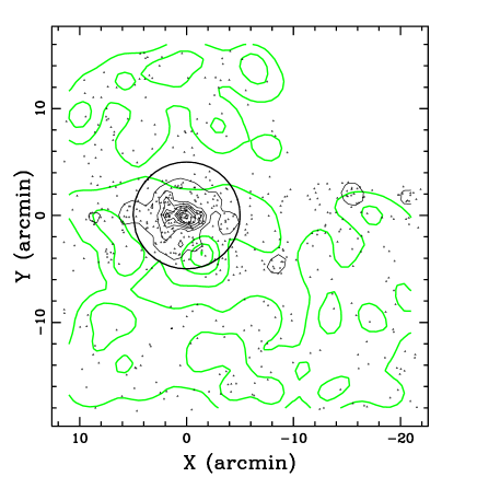
Figure 7: Spatial distribution on the sky and relative isodensity contour map of 582 likely cluster members (according to the colour–magnitude relation) with $R\leq 21$, obtained with the DEDICA method (black lines). For comparison we show the contour map of the 563 likely non-cluster members (grey lines). The plot is centred on the cluster centre. The circle indicates the 5$\mathrm{{}^{\prime}}\;$central region.

When analysing the 2D galaxy distribution for magnitude intervals the bimodal structure in the central cluster region is confirmed by the 141 galaxies brighter than 19 mag (in the $R$-band), while two samples of fainter galaxies (177 with $19<R\leq 20$ and 262 with $20<R\leq 21$) show only one significant peak closer to the W-peak than to the E-peak (see Figure 8).

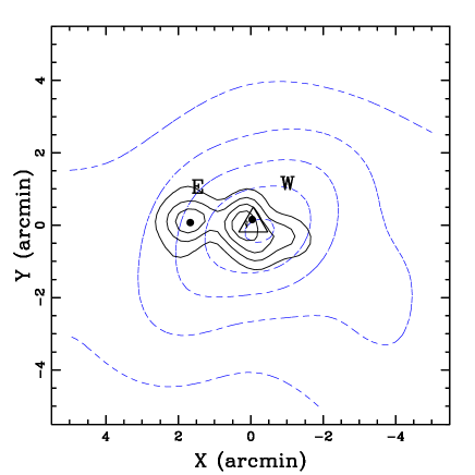
Figure 8: Isodensity contour map (zoomed within 1 $h_{70}^{-1}$ Mpc from the cluster centre) of likely cluster members of different magnitude intervals. For the sake of clarity we only show those for $R\leq 19$ and $19<R\leq 20$, indicated by black solid lines and dashed lines. We also indicate the position of the X-ray centre (large triangle), and the E- and W-peaks as recovered from galaxies having redshifts (small dots, see also Fig. 5).

3.4 3D structure of A773

The existence of correlations between positions and velocities of cluster galaxies is a footprint of real substructures.

In the case of A773 the standard approaches to determine these correlations fail (e.g. Boschin et al. bos06 (2006); Girardi et al. gir06 (2006)). In fact, we find no significant velocity gradient, no significant substructure according to the method by Dressler & Schectman (dre88 (1988)), and the result of the 3D KMM method is fully driven by the velocity-variable making us obtain again the two-group partition of Section 3.2.

As an alternative approach, we analyse the 2D distributions of the two groups determined using the velocity distribution. We compare the 2D distribution of the galaxies assigned to the LV-group (hereafter LV-galaxies) with that of the galaxies assigned to the HV-group (hereafter HV–galaxies) finding no significant difference according to the 2D Kolmogorov–Smirnov tests (2DKS test, see Fasano & Franceschini fas87 (1987) as implemented by Press et al. pre92 (1992)).

To go deeper into the question we also use the 2D DEDICA method. We find that the distribution of LV-galaxies shows a main, very significant peak located close to the W-peak, while the main 2D peak of the distribution of HV-galaxies is closely located near the E-peak, thus indicating a relation between velocity structure and 2D structure detected in the above two sections (see Fig. 9).

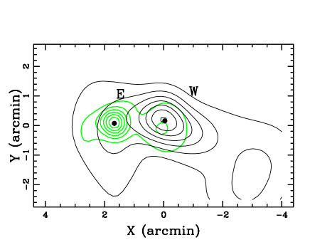
Figure 9: Comparison of isodensity contour maps recovered from the galaxies assigned to the low velocity peak (black solid line) and from galaxies assigned to the high velocity peak (light grey line). The position of peaks W and E are indicated by solid circles.

Moreover, the distribution of HV-galaxies also shows a secondary peak closely located near the W-peak. This secondary peak is only 93% significant and much less dense with respect to the main one (only 30%), but contains a similar number of galaxies (seven vs. eight). This secondary peak is also found when we consider only the 22 galaxies with a velocity higher than the peak velocity of $67453$ km s${}^{-1}\;$and therefore we exclude the possibility that the 2D secondary peak is induced by the difficulties in member assignment between the two velocity peaks (see Sect. 3.2). The likely conclusion is that some HV-galaxies are really connected with the high velocity D2 galaxy located in the region of the W-peak.

As a final approach, we analyse the velocity distributions of the galaxy populations located in the regions of the E- and W-peaks. Following Girardi et al. (gir05 (2005)) we analyse the profiles of mean velocity and velocity dispersion of galaxy systems corresponding to the E- and W-peaks to attempt an independent analysis.

In the case of the E-peak the integral $\sigma_{\rm v}$ profile shows a sharp increase starting from the peak centre (see Fig. 10). This is probably due to the contamination of a galaxy clump with a different mean velocity (see also Girardi et al. gir96 (1996) in the case of A3391–A3395). To avoid possible problems of contamination we decide to consider a sample E-sub formed by only the first five galaxies closest to the E-peak. In the case of the W-peak the value of $\sigma_{\rm v}$ computed using the first five galaxies is enough high – $\sim 1200$ km s${}^{-1}\;$– and the integral $\sigma_{\rm v}$ profile shows an almost stable behaviour out to $\sim$0.2 $h_{70}^{-1}$ Mpc , where it starts to increase (see Fig. 11). We decided to consider a sample W-sub formed by the first fourteen galaxies closest to the W-peak.

Table 2 lists kinematic properties for E- and W-subs and shows that these groups have similar properties of the HV-subcluster and of the whole cluster, respectively. When comparing the kinematics of E-sub and W-sub we find that their velocity distributions are different at the 97.8% c.l. according to the KS test (e.g. Ledermann led82 (1982), as implemented by Press et al. pre92 (1992) for small samples), and that the mean velocity and the velocity dispersion differ at the 99.6% c.l and 93.5% c.l. according to the means test and F test, respectively (e.g. Press et al. pre92 (1992)). Moreover, W-sub has a complex structure since its velocity distribution shows two peaks according to DEDICA (see the small upper-right panel of Fig. 11). The low velocity peak (LV-W-sub) contains the D1 galaxy and resembles the mean velocity of LV-subcluster. The high velocity peak (HV-W-sub) contains the D2 galaxy and resembles the mean velocity of HV-subcluster.

Figure 10: Kinematic profiles of the cluster obtained assuming the E-peak as centre. The vertical line indicates the region which encloses the galaxies of E-sub (see text). Differential (big circles) and integral (small points) mean velocity and LOS velocity dispersion profiles are shown in top and bottom panels, respectively. For the differential profiles are plotted the values obtained binning galaxies 10 by 10. For the integral profiles, the mean and dispersion at a given (projected) radius from the position of the E-peak is estimated by considering all galaxies within that radius: the first point refers to the first five galaxies and the last point refer to all galaxies contained in the cluster. The error bands at the $68\%$ c.l. are also shown.

Figure 11: The same as in Fig. 10, but referring to the W-peak. The small upper-right panel shows the velocity galaxy density (in normalized units), as provided by DEDICA for the galaxies of W-sub, i.e. those galaxies contained within the radius indicated by the vertical line.

3.5 Further insights using galaxy populations

In the case of A773, strongly substructured, the analysis of red and/or bright galaxies might be useful to trace the cores of the subclusters (e.g. Lubin et al. lub00 (2000); Boschin et al. bos04 (2004)). Moreover, active star forming galaxies might be related to the cluster–cluster merging phenomena (e.g. Bekki bek99 (1999)).

We divide the sample (99 galaxies having magnitudes) into low- and high-luminosity subsamples, each with 49 galaxies, by using the median $R$ magnitude = 19.08. The two subsamples do not differ in their velocity distribution according to the KS test and both show a bimodal velocity distribution according to the DEDICA method. In agreement with the photometric sample results, luminous galaxies clearly show the presence of both E and W peaks (see Figure 12).

Figure 12: Spatial distribution on the sky of 100 cluster members. More and less luminous galaxies are denoted by circles and crosses, respectively. The contour map recovered from the most luminous galaxies is also shown. The position of peaks W and E are indicated by solid, small circles.

Butcher & Oemler (but84 (1984)) define as “blue” those galaxies with rest-frame $B-V$ colours at least 0.2 mag bluer than that of the CMR, this translates to 0.447 mag for $B-R$ colours at $z\sim 0.21$ (see Mercurio et al. mer04 (2004) and Haines et al. hai04 (2004) for A209), and a comparable result is obtained by using the tables of Fukugita et al. (fuk95 (1995)). Therefore, we hereafter define $(B-R)_{\rm corr}=(B-R)-(3.507-0.072\times R)$ and “blue” those galaxies with $(B-R)_{\rm corr}<-0.45$, i.e. those with observed $B-V$ colours at least 0.45 mag bluer than that of the CMR. To analyse the colour segregation we also divide other galaxies into “red” [$-0.45\leq(B-R)_{\rm corr}\leq 0$] and “very red” [$(B-R)_{\rm corr}>0$]. We obtain three subsamples of 43 very red, 39 red, and 17 blue galaxies (see Fig. 6). The subsample of the very red galaxies shows two distinct peaks in the velocity distribution (LV–very red and HV–very red, see Table 2). When analysing the 2D galaxy distribution of each subsample through the DEDICA method we find that the very red galaxies show a significant peak at the position of the W-peak – this is true for both LV–very red and HV–very red subsamples separately – while red galaxies show a significant peak at the position of the E-peak (see Fig. 13). The blue galaxies are instead preferentially located towards western regions of the cluster.

Figure 13: Spatial distribution on the sky of 100 cluster members. Very red, red and and blue galaxies are denoted by crosses, circles and solid squares, respectively. The contour map recovered from the very red galaxies is also shown. The position of peaks W and E are indicated by solid small circles.

Finally, we consider galaxies of different spectral types. Of 76 classified member galaxies, we find 60 “passive” k-galaxies and 16 “active” galaxies, of which 10 are emission line galaxies (i.e. 5:1:1:3:1:5 for k+a:a+k:e(c)/e(c?):e(a)/e(a?):e(b):e, respectively). Both passive and emission line galaxy populations show the characteristic bimodal velocity distribution and have similar mean velocity and velocity dispersion, quite comparable to that of the whole sample. As for the 2D distribution, the passive population shows the characteristic bimodal distribution with the E- and W-peaks, while the active populations avoid these regions of high density. In particular, Fig. 14 shows that emission line galaxies are preferentially located towards south-western regions of the cluster. Indeed, we find that passive galaxies differ from the emission-line galaxies at the 98.0% c.l., respectively, according to the 2DKS test and despite some categories drawn in Fig. 14 include small numbers of objects and make this comparison difficult.

Figure 14: Spatial distribution on the sky of 100 cluster members. Large symbols denote spectroscopically classified galaxies: circles, squares, solid triangles, solid squares and solid pentagons indicate k,k+a/a+k,e(c)/e(c?),e(a)/e(a?) and e(b), respectively. Small dots indicate unclassified members.

4 X-ray analysis

X-ray analysis of A773 has already been performed in the past, both based on ROSAT (Pierre & Starck pie98 (1998), Rizza et al. riz98 (1998), Govoni et al. 2001b ) and Chandra data (Govoni et al. gov04 (2004)). In particular, Govoni et al. (gov04 (2004)) analysed two Chandra ACIS-I observations (exposures ID #533 and #3588). The two pointings have a clean total exposure time of 18.7 ks (see their table 1). More recently, Chandra has again observed A773 (exposure ID #5006). This pointing has an exposure time of 20.1 ks. In this section we propose an analysis of this Chandra ACIS-I observation.

Data reduction is performed using the package CIAO (Chandra Interactive Analysis of Observations) on chip I3 (field of view $\sim 8.5\arcmin\times 8.5\arcmin$). First, we remove events from the level 2 event list with a status not equal to zero and with grades one, five and seven. We then select all events with energy between 0.3 and 10 keV. In addition, we clean bad offsets and examine the data, filtering out bad columns and removing times when the count rate exceeds three standard deviations from the mean count rate per 3.3 s interval. We then clean the I3 chip for flickering pixels, i.e. times where a pixel has events in two sequential 3.3 s intervals. The resulting exposure time for the reduced data is 19.6 ks.

In Fig. 2 we plot an $R$-band image of the cluster with superimposed the X-ray contour levels of the Chandra image. The shape of the cluster appears to be moderately elliptical. By using the CIAO package Sherpa we fit an elliptical 2D Beta model to the X-ray photon distribution to quantify the departure from the spherical shape. The model is defined as follows:

$$f(x,y)=f(r)=A/[1+(r/r_{0})^{2}]^{\alpha},$$ (1)

where the radial coordinate $r$ is defined as $r(x,y)=[X^{2}(1-\epsilon)^{2}+Y^{2}]^{1/2}/(1-\epsilon)$, $X=(x-x_{0})\,\cos\,\theta+(y-y_{0})\,\sin\,\theta$ and $Y=(y-y_{0})\,\cos\,\theta-(x-x_{0})\,\sin\,\theta$. Here $x$ and $y$ are physical pixel coordinates on chip I3. The best fit centroid position is located very close to the dominant galaxy D1, i.e. R.A.=$09^{\mathrm{h}}17^{\mathrm{m}}52\,\hbox to0.0pt{\hbox{$\mathrm{{}^{s}}$}\hss}{\hbox{$.$}}\,87$, Dec.=$+51\mathrm{{}^{\circ}}43\mathrm{{}^{\prime}}39\,\hbox to0.0pt{\hbox{$\mathrm{{}^{\prime}\hskip-1.00006pt{}^{\prime}}$}\hss}{\hbox{$.$}}\,2$ (J2000.0). The best-fit core radius, the ellipticity and the position angle are $r_{0}=47\pm$3 arcsec (167$\pm$11 $h_{70}^{-1}$ kpc), $\epsilon=0.23\pm$0.02 and PA=79.7$\pm$2.8 degrees (measured counterclockwise from the north), respectively.

Isophotes in Fig. 2 suggest that the core of A773 is substructured with two distinct maxima in the surface brightness distribution. The presence of these two peaks is confirmed by a wavelet analysis of the image performed by the task CIAO/Wavdetect. The task was run on several scales to search for substructures with different sizes. The significance threshold was set at $10^{-6}$. The results are shown in Fig. 2. Green ellipses represent two significant surface brightness peaks found by Wavdetect in the core of the cluster. They are located at R.A. $09^{\mathrm{h}}\,17^{\mathrm{m}}\,53.4^{\mathrm{s}}$ and Dec. $+51\degr\,43\arcmin\,44\arcsec$, and at R.A. $09^{\mathrm{h}}\,17^{\mathrm{m}}\,51.4^{\mathrm{s}}$ and Dec. $+51\degr\,43\arcmin\,32\arcsec$, respectively. This finding confirms the results of Pierre & Stark (pie98 (1998)) and Rizza et al. (riz98 (1998)), who first noted the complex structure of the core from a 16 ks ROSAT/HRI exposure.

For the spectral analysis of the cluster X-ray photons, we compute a global estimate of the ICM temperature. The temperature is computed from the spectrum of the cluster within a circular aperture of 2$\arcmin$ radius around the cluster centre. Fixing the absorbing galactic hydrogen column density at 1.44$\times$10²⁰ cm^-2, computed from the HI maps by Dickey & Lockman (dic90 (1990)), we fit a Raymond–Smith (ray77 (1977)) spectrum using the CIAO package Sherpa with a $\chi^{2}$ statistics. Considering the energy range 0.8–10 keV, we find a best fit temperature of $T_{\rm X}=\,$7.8 $\pm\,0.4$ keV and a metal abundance of 0.34$\pm\,0.07$ solar, in agreement with the results of Govoni et al. (gov04 (2004)).

5 Discussion

The global LOS velocity dispersion $\sigma_{\rm v}=1394_{-68}^{+84}$ km s${}^{-1}\;$is considerably higher than the average X-ray temperature $T_{\rm X}=$7.8$\pm$0.4 keV from our analysis of Chandra data when assuming the equipartition of energy density between gas and galaxies (i.e. $\beta_{\rm spec}=1.51^{+0.13}_{-0.10}$ to be compared with $\beta_{\rm spec}=1$). This suggests that the cluster is far from dynamical equilibrium and indeed we do find evidence that A773 shows two peaks both in the velocity space ($\Delta{\rm v}\sim 2800$ km s^-1) and in the 2D projected position space ($\sim 2\arcmin\,$ between the E-peak and the W-peak).

The main subsystem is detected as the LV-peak in the velocity distribution, has a velocity dispersion of $\sigma_{{\rm v},{\rm c}}$=800–1100 km s${}^{-1}\;$ – comparable to massive clusters - and its centre probably coincides with the D1 galaxy, located close to the main 2D peak (W-peak) and the peak of X-ray emission. The distribution of very red galaxies is also peaked in the same place. Both the low velocity galaxies located close to the W-peak (LV-W-sub) and the low velocity, very red galaxies (LV-very red) show a $\sigma_{\rm v}$ value of about 500 km s^-1, lower than the global sigma as often observed in the case of a core cluster, in particular when examining passive galaxies (Adami et al. ada98 (1998); Biviano & Katgert biv04 (2004)).

A secondary subsystem is detected as the HV-peak in the velocity distribution and has a moderate velocity dispersion of $\sigma_{{\rm v},{\rm g}}\sim 500$ km s^-1. Its spatial structure is rather complex, showing two galaxy concentrations, one at the location of the E-peak and the other at the location of the W-peak, i.e. close to the high velocity, D2 dominant galaxy (see Fig. 9 and the upper-right panel of Fig. 11). The absence of a concentration of very red galaxies and of any close X-ray peak, as well as the presence of only a minor DM peak (Dahle et al. dah02 (2002)), suggest that the E-peak is dynamically of minor importance. Analysing galaxies around the two concentrations (E-sub and HV-W-sub) we find similar kinematic properties; thus, with present data we cannot distinguish whether they are two independent galaxy groups or two components of the same group. In favour of the first hypothesis, we notice that both theoretical predictions and observational data suggest that clusters are formed by numerous small infalling systems (see the case of A85-A87 complex in Durret et al. dur98 (1998)). In this case, the similarity of the mean velocities of E-sub and HV-W-sub might reflect that their velocities are of dynamical origin, both groups strongly interacting with the same cluster potential and thus having a similar merging velocity. In the case of the second hypothesis, E-sub could be either a dense substructure of the HV-system or a part of the core of the HV-system dynamically decoupled from the dominant galaxy during the cluster merger. We notice that Adami et al. (ada05 (2005)) found a similar feature in the Coma cluster, where the N03–SW group has the same mean velocity as NGC 4889, one of the two dominant galaxies, even if it is spatially distant in 2D.

5.1 A773 mass estimate

On the basis of the above discussion we estimate the mass of A773, assuming that the system is formed by a main cluster with a velocity dispersion of $\sigma_{{\rm v},{\rm c}}$=800–1100 km s${}^{-1}\;$and one or two groups with $\sigma_{{\rm v},{\rm g}}\sim 500$ km s^-1. Here we report our results in the case of one group, but notice that in the case of two groups, they have the same virial masses and the results of this section are still valid.

Although the system is probably in a phase of strong interaction (see also the following section) so that the subsystems are still detectable in the velocity distribution, let us assume having a good estimate of $\sigma_{\rm v}$ of the subsystems before the merger. To apply the virial method we must assume that each subsystem is in dynamical equilibrium. This might be not true in the case of a possibly substructured group (see above). On the other hand, the mass estimate of the whole complex depends above all on the main subsystem. whose structure is much more regular.

Following the prescriptions of Girardi & Mezzetti (gir01 (2001)), we assume for the radius of the quasi-virialized region R${}_{\rm vir,c}=0.17\times\sigma_{\rm v}/H(z)=2.3$-3.2 $h_{70}^{-1}$ Mpc and R${}_{\rm vir,g}=0.17\times\sigma_{\rm v}/H(z)\sim 1.4$ $h_{70}^{-1}$ Mpc for the cluster and the group, respectively – see their eq. 1 after introducing the scaling with $H(z)$ (see also eq.  8 of Carlberg et al. car97 (1997) for R₂₀₀). Therefore, our spectroscopic catalogue samples the whole group virialized region and more than half of the cluster one.

One can compute the mass using the virial theorem (Limber & Mathews lim60 (1960); see also, for example, Girardi et al. gir98 (1998)) under the assumption that mass follows galaxy distribution: $M=M_{\rm svir}-\rm{SPT}$, where $M_{\rm svir}=3\pi/2\cdot\sigma_{\rm v}^{2}{\rm R}_{\rm PV}/G$ is the standard virial mass, R_PV a projected radius (equal two times the harmonic radius), and SPT is the surface pressure term correction (The & White the86 (1986)). The estimate of $\sigma_{\rm v}$ is generally robust when computed within a large cluster region (see Fig. 5 of Girardi et al. gir06 (2006) and Fadda et al. fad96 (1996) for other examples), hence for each of the two subsystems we consider the corresponding above-global values $\sigma_{{\rm v},{\rm c}}$ and $\sigma_{{\rm v},{\rm g}}$. The value of R_PV depends on the size of the region considered so that the computed mass increases (but not linearly) with the increasing region considered. Since the two subsystems are partially aligned along the LOS we avoid computing R_PV by using data for observed galaxies and use an alternative estimate that was shown to be good when R_PV is computed within R_vir (see eq. 13 of Girardi et al. gir98 (1998)). This alternative estimate is based on our knowledge of the galaxy distribution and, in particular, a galaxy King-like distribution with parameters typical of nearby/medium-redshift clusters: a core radius R${}_{\rm core}=1/20\times{\rm R}_{\rm vir}$ and a slope-parameter $\beta_{\rm fit}=0.8$, i.e. the volume galaxy density at large radii as $r^{-3\beta_{\rm fit}}=r^{-2.4}$ (Girardi & Mezzetti gir01 (2001)). For the whole virialized region we obtain R${}_{\rm PV,c}=1.7$-2.4 $h_{70}^{-1}$ Mpc and R${}_{\rm PV,g}\sim 1.4$ $h_{70}^{-1}$ Mpc , where a 25% error is expected because typical, rather than individual, galaxy distribution parameters are assumed. As for the SPT correction, we assume a 20% one, computed combining data on many clusters (e.g. Carlberg et al. car97 (1997); Girardi et al. gir98 (1998)). This leads to virial masses for the subsystems of $M_{\rm c}(<{\rm R}_{\rm vir,c}=2.3-3.2\,\;h_{70}^{-1}\mathrm{Mpc})=1.0$-2.5 $\times 10^{15}\;h_{70}^{-1}\;M_{\odot}\;$of $M_{\rm g}(<{\rm R}_{\rm vir,g}=1.4\,\;h_{70}^{-1}\mathrm{Mpc})\sim 2.4$ $\times 10^{14}\;h_{70}^{-1}\;M_{\odot}\;$with a typical error of $\sim$30%. A reliable mass estimate of the whole system is then $M=1.2$–2.7 $\times 10^{15}\;h_{70}^{-1}\;M_{\odot}$, in agreement with rich clusters reported in the literature (e.g. Girardi et al. gir98 (1998); Girardi & Mezzetti gir01 (2001)).

To compare our result with the estimate obtained via gravitational lensing we obtain a projected mass assuming that the cluster is described by a King-like mass distribution (see above), or a NFW profile where the mass-dependent concentration parameter is taken from Navarro et al. (nav97 (1997)) and rescaled by the factor $1+z$ (Bullock et al. bul01 (2001); Dolag et al. dol04 (2004)). Moreover, we assume that the two subsystems have coincident centres, and that the subsystems themselves are extended only to one R_vir. We obtain $M_{\rm proj}(<\rm{R}=90$$\mathrm{{}^{\prime}}\hskip-1.00006pt\mathrm{{}^{\prime}}$)=(4.4–7.9)$\times 10^{14}\;h_{70}^{-1}\;M_{\odot}\;$in agreement with that found by Dahle et al. (dah02 (2002)) considering the quoted errors ($M_{\rm Dahle}\sim 3$$\times 10^{14}\;h_{70}^{-1}\;M_{\odot}\;$with an upper error of the 50% after rescaling to our cosmological model).

Using the same mass distributions we compute $M(<\rm{R}=1$ $h_{70}^{-1}$ Mpc)=(5.9–11.1)$\times 10^{14}\;h_{70}^{-1}\;M_{\odot}\;$and, using $r$-band luminosity by Popesso et al. (pop04 (2004)), estimate $M/L$=(150–280) $h_{70}\;M_{\odot}/L_{\odot}$. The upper value is typical of clusters of similar redshift (Carlberg et al. car96 (1996)).

5.2 Merging scenario

The X-ray emission shows two very close peaks along the NE–SW direction separated by $\sim$0.5^′. The main X-ray peak, the NE one, is closely located near – but is not coincident with – the D1 galaxy. The secondary, SW, one does not coincide with any luminous galaxy or obvious galaxy substructure (see Fig. 2). This lack of correlation between collisional and non-collisional components strongly suggests that the cluster is undergoing an advanced phase of merging (e.g. Roettiger et al. roe97 (1997)). Moreover, the direction of elongation of the isophotes of the X-ray emission (NEE–SWW direction, PA$\sim$80 degrees) is similar to that indicated by the elongation of galaxy distribution (see, for example, contours for very red galaxies in Fig. 13), but quite different from N–S one indicated by the two dominant galaxies and the elongation of the main DM clump (Dahle et al. dah02 (2002)). It is worth noting that the literature reports several cases of clusters having two dominant galaxies with significantly different velocities, where the elongation of the X-ray emission is rotated from the axis connecting the two dominants and/or with X-ray peaks not coinciding with the location of the dominants (e.g. A2255 by Burns et al. bur94 (1994); RXJ1314-25 by Valtchanov et al. val02 (2002); A2744 by Boschin et al. bos06 (2006)). On smaller scales, A773 also shows minor but intriguing features. The E-group is not really aligned with the direction of the elongation of the X-ray emission, but rather shows a PA $\sim$ 90 degrees with respect to the cluster centre. Moreover, although the main DM peak roughly coincides with that indicated by the two dominant galaxies, it indeed is offset by about 1^′.

Further support in favour of an advanced phase of merging comes from the luminosity segregations. Although both luminous and faint galaxies show two peaks in their velocity distribution, only the luminous ones show the E-peak in the 2D distribution. Indeed, it is not unusual that galaxies of different luminosity trace the dynamics of cluster mergers in a different way. The first evidence was given by Biviano et al. (biv96 (1996); see also Mercurio et al. mer03 (2003)), who found that the two central dominant galaxies of the Coma cluster are surrounded by luminous galaxies accompanied by the two main X-ray peaks, while the distribution of faint galaxies tend to form a structure not centred on one of the two dominant galaxies but rather coincident with a secondary peak detected in X-rays. Therefore, following Biviano et al. (biv96 (1996)), we might speculate that the merging is in an advanced phase, where faint galaxies trace the forming structure of the cluster, while more luminous galaxies still trace the remnants of pre-merging clumps, which could be so dense to survive for a long time after the merging (as suggested by numerical simulations; see González–Casado et al. gon94 (1994)).

As discussed in the above sections, the subsystems involved in the merger are one cluster and one or two groups with a large mass ratio from 4:1 to 10:1, depending on which $\sigma_{\rm v}$ estimate we use for the cluster, with a velocity separation that ranges $2100-2500$ km s${}^{-1}\;$in the cluster rest-frame. Cosmological simulations suggest that these high impact velocities might be occurring in phenomena of cluster merging (e.g. Crone & Geller cro95 (1995)). The value of a merging velocity of $\sim 3000$ km s${}^{-1}\;$is also predicted by $N$-body numerical simulations of Pinkney et al. (pin96 (1996)) and is probably associated with the phase of the core crossing in a cluster–cluster merging process. In the case of A773, the extremely large LOS component of the velocity indicates that the LOS is close to the merging axis.

As for the direction of the merger, the elongations noted in the X-ray emission, the galaxy and DM distributions indicate that the merger is not occurring entirely along the LOS, but must have at least a small transverse component in the plane of the sky. However, since the variety of features do not indicate a unique direction we conclude that the geometry of the merger is very complex. The likely scenario is that we are looking at a multiple merger where the N–S direction might indicate the direction of an older merger event concerning the cluster and the group associated with the D2 dominant galaxy. D1 and D2 might be the tracers of the two cores destined to oscillate around the mean velocity for a long time (i.e. from two to several $10^{9}$ yr as suggested by numerical simulations; see, for example, Nakamura et al. nak95 (1995); Faltenbacher et al. fal06 (2006)). In fact, a high velocity difference between the two dominant galaxies is often suggestive of an energetic cluster merger (e.g. Burns et al. bur95 (1995)) and this process is thought to be the cause of the formation of dumbbell galaxies in a few merging clusters (e.g. Beers et al. bee92 (1992); Flores et al. flo00 (2000)). The NE by E–SW by W elongation of the X-ray emission might indicate the direction of a more recent merger event concerning the eastern group (i.e. that centred on the E-peak). We are probably seeing this merging after the phase of the core passage. This might explain the offset of the centre of the X-ray emission, the offset of the DM peak and the small deviation of the eastern group from the initial NE by E–SW by W direction. In this case, the eastern group would have shed its gas as a result of ram pressure at the entry into the main cluster at its SW by W side and, in fact, we do not see any eastern peak in X-ray emission (a scenario already suggested by Govoni et al. gov04 (2004)). Further support for this scenario comes from the fact that emission line galaxies are preferentially located in the SW cluster region, the starbursts possibly being induced by the infalling subcluster (e.g. Bekki bek99 (1999)).

One expects that cluster mergers will drive shock waves into the intracluster gas of the two subclusters (see Sarazin sar02 (2002) for a review). The Mach number of the shock is $\cal M$=${\rm v}_{\rm s}/c_{\rm s}$, where ${\rm v}_{\rm s}$ is the velocity of the shock and $c_{\rm s}$ is the sound speed in the preshock gas. In the stationary regime we can assume that ${\rm v}_{\rm s}$ is the merger velocity, i.e. ${\rm v}_{\rm s}\mathrel{\hbox{\hbox to0.0pt{\hbox{\lower 4.0pt\hbox{$\sim$}}\hss}\hbox{$>$}}}2300$ km s${}^{-1}\;$taking into account the projection factor. We obtain $c_{\rm s}\mathrel{\hbox{\hbox to0.0pt{\hbox{\lower 4.0pt\hbox{$\sim$}}\hss}\hbox{$<$}}}1134$ km s${}^{-1}\;$from the thermal velocity, i.e. from the observed $T_{\rm X}$ converted into velocity using the usual equipartition of energy density between gas and galaxies (see Sect. 5) and taking into account that the observed $T_{\rm X}$ might be enhanced with respect to pre-merging values. We therefore estimate $\cal M$ $\mathrel{\hbox{\hbox to0.0pt{\hbox{\lower 4.0pt\hbox{$\sim$}}\hss}\hbox{$>$}}}2.0$. According to our merging scenario, this value of $\cal M$ would make front or bow shocks possibly detectable in X-ray observations. However, in the case of the LOS being very close to the merger axis, a front shock would expand in an almost parallel direction to the LOS. So because of the geometry of the problem we can only observe a global enhancement of the X-ray temperature in the whole cluster. To date, the observational picture is inconclusive. Govoni et al. (gov04 (2004)) found a very hot region in the western cluster region, but, analysing a slightly larger and more homogeneous amount of data, we find no significant variation in the X-ray temperature.

As for the comparison with the radio halo feature, its emission is somewhat displaced towards the E-peak (see Fig. 2 and Govoni et al. gov04 (2004)). This is a suggestive indication in favour of the connection between cluster mergers and radio halos. Recent calculations (Cassano & Brunetti cas05 (2005)) show that a fraction $\sim$10% of the thermal-cluster energy may be channeled in the form of turbulence in case of main (i.e. mass ratio$\leq$ 3:1) cluster mergers and this may power up radio halos. However, a typical massive cluster is formed by a series of minor mergers and a minor merger may still power the particle acceleration process especially if they happen in clusters which are already dynamically disturbed by precedent mergers (see Fig. 2 and the time-evolution of the acceleration coefficient in Fig. 5 in Cassano & Brunetti cas05 (2005)). This is probably the case of A773.

5.3 LSS structure

We also analyse the large scale structure (LSS) surrounding A773 since the merging direction was shown to be frequently correlated with the supercluster environment (e.g. Durret et al. dur98 (1998); Arnaud et al. arn00 (2000)). We find three Abell clusters within a circle of 2 degrees centred on A773: A782 of richness class $R=2$ and A746 and A793 of richness class $R=1$. The closest one, A782 at 40.6^′, has five galaxies with known redshift at 0.20–021 within a circle of 5$\mathrm{{}^{\prime}}\;$as recovered by using NED; we therefore assume a cluster redshift of 0.21. Assuming the respective redshifts, the distance of A782 to A773 is $\sim 40$ $h_{70}^{-1}$ Mpc thus comparable to the typical sizes of superclusters (e.g. Batuski & Burns bat85 (1985); Zucca et al. zuc93 (1993)). The direction of A782 is indicated in Figure 2: the result is that the direction of the elongation of X-ray emission and the direction indicated by the eastern group are $\sim 10$–20 degrees different with the axis A773/A782. Therefore, we speculate that A773 and A782 lie along the same LSS filament where the eastern group also originated. In this case, to take into account the geometry of the problem and the relative velocity difference of the eastern group and the main system, the eastern group lies in front of A773 and has already reached the turnaround point, with a second centre passage no incipient.

6 Summary and conclusions

We present the results of a dynamical analysis of the rich, X-ray luminous and hot cluster of galaxies A773 containing a diffuse radio halo.

Our analysis is based on new redshift data for 142 galaxies, measured from 107 spectra obtained at the TNG and 37 spectra recovered from the CFHT archive in a cluster region within a radius of $\sim 1.8$ $h_{70}^{-1}$ Mpc from the cluster centre. We also use new photometric data obtained at the INT in a field larger than 30^′$\times$30$\mathrm{{}^{\prime}}\;$.

We select 100 cluster members with $62250<{\rm v}<68850$ km s^-1and compute a global LOS velocity dispersion of galaxies, $\sigma_{\rm v}=1394_{-68}^{+84}$ km s^-1.

The 2D distribution shows two significant peaks separated by $\sim$2$\mathrm{{}^{\prime}}\;$along the EW direction with the main, western one located close to the position of the two dominant galaxies and the X-ray peak. The velocity distribution of cluster galaxies shows two peaks at ${\rm v}\sim$65000 and $\sim$67500 km s^-1, corresponding to the velocities of the two dominant galaxies. The low velocity structure has high velocity dispersion – $\sigma_{\rm v}=800-1100$ km s${}^{-1}\;$– and its galaxies are centred on the western 2D peak. The high velocity structure has intermediate velocity dispersion – $\sigma_{\rm v}\sim 500$ km s${}^{-1}\;$– and is characterized by a complex 2D structure with a component centred on the western 2D peak and a component centred on the eastern 2D peak, these components probably being two independent groups.

Other evidence that A773 is dynamically disturbed comes from 1) the presence of two X-ray peaks in the X-ray emission in the central cluster region, offset with respect to possible optical counterparts; 2) the elongation of X-ray emission (PA$\sim$80 degrees) along the NE by E–SW by W direction, while the two dominant galaxies indicate a N–S direction; 3) the preferential SW location of emission line galaxies.

According to our likely scenario the high velocity group surrounding the high velocity dominant galaxies traces an old merger of the main cluster with a group along the N–S direction, while the high velocity group surrounding the eastern 2D peak of galaxies indicates a more recent merger, but already enough advanced, along the NE by E-SW by W direction. Acting on an already dynamically disturbed cluster, this second merger event would be the likely cause of a very complex observational picture and of the radio halo, which is somewhat displaced towards the eastern group.

For the whole galaxy complex we estimate a virial mass $M=1.2$–2.7 $\times 10^{15}\;h_{70}^{-1}\;M_{\odot}\;$and $M(<1$ $h_{70}^{-1}$ Mpc)=(5.9–11.1)$\times 10^{14}\;h_{70}^{-1}\;M_{\odot}$, values comparable to those of other rich clusters at nearby or moderate redshifts.

Table 3: Velocity catalog of 142 spectroscopically measured galaxies. In Column 1, IDs in italics indicate non–cluster galaxies. IDs 59 and 60 indicate the two dominant galaxies (D1 and D2, respectively).

$$\begin{array}[]{r c c c c r c}\hline\cr\vskip 3.0pt plus 1.0pt minus 1.0pt\cr\hline\cr\vskip 3.0pt plus 1.0pt minus 1.0pt\cr\mathrm{ID}&\mathrm{\alpha},\mathrm{\delta}\,(\mathrm{J}2000)&\mathrm{B}&\mathrm{R}&\mathrm{v}&\mathrm{\Delta}\mathrm{v}&\mathrm{SC}\\ &09^{h},+51^{o}&&&\,\,\,\,\,\,\,\mathrm{(\,km}&\mathrm{s^{-1}\,)}&\\ \hline\cr\vskip 3.0pt plus 1.0pt minus 1.0pt\cr\textit{1}&17\ 00.60,42\ 52.6&19.77&18.36&34762&70&\rm{e(c)}\\ 2&17\ 06.58,44\ 07.1&20.54&18.86&64233&105&\\ \textit{3}&17\ 13.85,43\ 17.0&22.05&19.88&132256&93&\\ 4&17\ 14.04,43\ 38.6&21.24&19.29&63970&99&\rm{k+a}\\ 5&17\ 14.50,43\ 28.2&21.73&20.46&65568&123&\\ \textit{6}&17\ 17.21,44\ 43.4&22.72&19.95&132667&76&\\ 7&17\ 19.80,38\ 48.8&21.38&19.39&68615&147&\\ 8&17\ 20.86,38\ 45.2&19.63&18.19&68559&94&\rm{e(a)}\\ 9&17\ 22.99,41\ 18.6&22.50&20.17&64925&236&\\ 10&17\ 23.14,40\ 51.6&22.46&20.09&65517&144&\\ 11&17\ 24.05,38\ 15.4&20.67&19.29&64503&87&\rm{e(a?)}\\ 12&17\ 26.59,43\ 40.4&21.00&19.47&62362&124&\\ \textit{13}&17\ 27.86,37\ 33.2&20.53&18.27&94246&76&\\ 14&17\ 28.73,42\ 23.0&21.30&19.28&62282&58&\rm{k}\\ 15&17\ 28.75,43\ 50.2&21.39&20.33&63859&86&\rm{e(b)}\\ \textit{16}&17\ 29.71,42\ 59.4&20.93&18.76&94885&76&\rm{e(c)}\\ 17&17\ 29.78,43\ 08.0&21.27&19.32&68655&118&\\ 18&17\ 31.66,44\ 43.1&21.81&20.34&68206&74&\\ 19&17\ 32.50,42\ 19.9&21.77&19.25&65171&111&\rm{e(c?)}\\ 20&17\ 32.57,42\ 22.2&22.21&20.72&64575&136&\\ 21&17\ 34.25,41\ 13.2&20.64&18.50&65848&69&\rm{k}\\ 22&17\ 35.02,44\ 32.6&22.06&19.73&67320&68&\\ 23&17\ 35.09,41\ 18.6&20.97&19.13&65309&86&\rm{k}\\ 24&17\ 35.38,38\ 39.8&20.44&18.73&63729&105&\rm{k+a}\\ 25&17\ 35.59,41\ 17.9&20.66&18.98&63067&99&\\ \textit{26}&17\ 36.10,44\ 18.2&20.75&19.44&58492&81&\\ 27&17\ 36.29,45\ 27.0&21.89&19.73&67997&87&\\ \textit{28}&17\ 37.08,42\ 53.6&22.26&19.87&93910&73&\\ 29&17\ 37.37,42\ 36.4&22.85&20.73&64940&212&\\ 30&17\ 37.99,44\ 17.5&20.22&18.08&66016&51&\rm{k}\\ 31&17\ 38.66,43\ 25.7&20.60&19.30&64889&85&\rm{e(a?)}\\ \textit{32}&17\ 38.74,46\ 58.4&19.67&18.84&20854&114&\rm{e(a?)}\\ 33&17\ 39.22,46\ 53.8&20.93&18.80&64216&118&\rm{k}\\ 34&17\ 39.48,41\ 49.6&21.97&20.20&67577&70&\\ 35&17\ 40.73,38\ 18.6&19.95&18.72&67396&86&\\ 36&17\ 40.80,41\ 31.6&22.54&20.13&65289&206&\\ \textit{37}&17\ 41.06,43\ 58.4&22.19&20.68&124666&24&\rm{e(c?)}\\ \textit{38}&17\ 42.79,43\ 41.2&20.90&19.77&55811&93&\rm{e(c)}\\ 39&17\ 44.04,40\ 21.0&22.51&20.52&67468&148&\rm{e(c?)}\\ 40&17\ 44.66,43\ 26.4&21.73&19.63&65758&70&\rm{k}\\ 41&17\ 45.72,42\ 55.1&21.66&19.52&64248&72&\rm{k}\\ 42&17\ 46.32,43\ 13.1&21.26&18.90&65547&50&\rm{k}\\ 43&17\ 46.85,45\ 29.5&20.74&18.64&65902&54&\rm{k}\\ 44&17\ 47.14,40\ 59.2&21.26&19.03&65661&106&\rm{k}\\ 45&17\ 48.02,46\ 35.4&20.30&18.65&66653&112&\rm{k}\\ 46&17\ 48.22,46\ 13.1&20.85&18.76&66848&60&\rm{k}\\ 47&17\ 48.62,43\ 43.7&22.07&20.81&64023&90&\\ \textit{48}&17\ 48.82,40\ 59.9&19.90&18.78&44429&81&\rm{e(a)}\\ \textit{49}&17\ 48.89,44\ 53.5&20.05&18.73&55538&92&\rm{e(a)}\\ 50&17\ 49.46,43\ 08.4&21.69&19.18&68830&76&\rm{k}\\ \vskip 3.0pt plus 1.0pt minus 1.0pt\cr\hline\cr\vskip 3.0pt plus 1.0pt minus 1.0pt\cr\hline\cr\end{array}$$

Table 3: Continued.

$$\begin{array}[]{r c c c c r c}\hline\cr\vskip 3.0pt plus 1.0pt minus 1.0pt\cr\hline\cr\vskip 3.0pt plus 1.0pt minus 1.0pt\cr\mathrm{ID}&\mathrm{\alpha},\mathrm{\delta}\,(\mathrm{J}2000)&\mathrm{B}&\mathrm{R}&\mathrm{v}&\mathrm{\Delta}\mathrm{v}&\mathrm{SC}\\ &09^{h},+51^{o}&&&\,\,\,\,\,\,\,\mathrm{(\,km}&\mathrm{s^{-1}\,)}&\\ \hline\cr\vskip 3.0pt plus 1.0pt minus 1.0pt\cr 51&17\ 49.66,41\ 04.9&19.88&17.64&65088&62&\rm{k}\\ 52&17\ 49.82,43\ 51.0&22.67&21.27&67857&58&\rm{e(c?)}\\ 53&17\ 50.54,43\ 26.4&20.95&18.63&63900&38&\rm{k}\\ 54&17\ 51.00,43\ 16.0&22.27&19.68&63696&64&\\ \textit{55}&17\ 51.96,41\ 33.7&20.13&19.04&114971&75&\rm{e(a)}\\ 56&17\ 52.56,43\ 50.2&20.84&18.31&64849&46&\rm{k}\\ 57&17\ 53.09,42\ 55.4&20.33&18.05&67364&72&\rm{k}\\ 58&17\ 53.16,44\ 08.9&20.81&18.59&64194&74&\rm{k}\\ 59&17\ 53.26,43\ 36.5&18.82&16.49&65131&50&\rm{k}\\ 60&17\ 53.33,44\ 00.6&18.93&16.73&67765&56&\rm{k}\\ 61&17\ 53.38,44\ 24.0&21.40&19.05&65152&124&\rm{k}\\ 62&17\ 54.17,43\ 27.5&21.26&18.87&67578&126&\rm{k}\\ 63&17\ 54.17,43\ 55.6&19.90&17.83&66477&28&\rm{k}\\ 64&17\ 54.24,44\ 52.8&20.44&18.58&68485&66&\rm{k}\\ \textit{65}&17\ 54.82,42\ 46.8&22.46&19.99&79178&158&\\ \textit{66}&17\ 54.84,47\ 03.8&18.84&17.77&21910&116&\rm{e(a)}\\ 67&17\ 55.54,43\ 54.1&20.77&18.49&66543&30&\rm{k}\\ \textit{68}&17\ 55.97,41\ 51.0&20.85&19.24&55993&87&\rm{e(c)}\\ 69&17\ 56.76,43\ 28.6&21.13&18.89&64437&57&\rm{k}\\ 70&17\ 57.10,46\ 10.9&21.20&19.00&68250&50&\rm{k}\\ 71&17\ 57.82,43\ 27.4&23.41&21.39&66885&130&\\ 72&17\ 58.20,41\ 35.5&21.01&18.59&67420&39&\rm{k}\\ 73&17\ 59.76,40\ 03.7&21.76&19.54&67738&64&\rm{k}\\ 74&18\ 00.14,46\ 23.2&21.24&19.12&68085&51&\rm{k}\\ 75&18\ 00.24,44\ 11.0&20.89&19.02&62377&46&\rm{k+a}\\ 76&18\ 00.60,44\ 07.4&21.30&18.86&64978&33&\rm{k}\\ 77&18\ 01.27,44\ 13.6&21.58&19.15&68682&69&\rm{k}\\ 78&18\ 01.37,42\ 25.9&21.54&19.24&66377&69&\rm{k}\\ 79&18\ 01.75,40\ 34.0&21.27&18.85&64829&72&\rm{k}\\ 80&18\ 02.86,40\ 07.3&21.58&19.55&63748&87&\rm{k}\\ 81&18\ 02.86,41\ 40.6&20.27&18.78&68358&44&\rm{a+k}\\ 82&18\ 03.46,43\ 51.2&20.20&17.98&67742&23&\rm{k}\\ 83&18\ 03.55,43\ 33.2&19.95&17.77&67969&54&\rm{k}\\ 84&18\ 03.77,43\ 28.2&21.29&19.24&66659&166&\\ 85&18\ 04.01,42\ 54.0&21.50&19.41&65774&66&\rm{k}\\ 86&18\ 04.10,43\ 12.7&21.05&18.76&64671&46&\rm{k}\\ 87&18\ 04.42,43\ 44.4&19.59&17.53&67673&36&\rm{k}\\ 88&18\ 05.06,43\ 49.8&20.04&17.98&67047&24&\rm{k}\\ 89&18\ 05.38,41\ 04.2&21.80&20.04&64928&112&\rm{e(a)}\\ 90&18\ 05.57,46\ 53.4&20.50&18.51&67098&52&\rm{k+a}\\ \textit{91}&18\ 05.64,39\ 59.0&21.46&19.38&12022&72&\\ 92&18\ 05.71,45\ 18.0&20.50&18.52&66287&66&\rm{e(c)}\\ 93&18\ 05.78,43\ 40.1&20.22&18.20&65414&24&\rm{k}\\ 94&18\ 06.22,42\ 00.0&20.90&18.91&66502&60&\rm{k}\\ 95&18\ 07.08,44\ 17.2&20.51&18.23&65081&27&\rm{k}\\ \textit{96}&18\ 07.27,49\ 13.8&19.56&18.44&44491&88&\rm{e(b)}\\ 97&18\ 08.57,43\ 42.6&21.16&18.98&67860&28&\rm{k}\\ \textit{98}&18\ 08.57,48\ 51.5&20.36&19.28&44498&70&\rm{e(c)}\\ 99&18\ 08.64,48\ 11.3&0.0&0.0&65850&70&\rm{k}\\ 100&18\ 09.79,41\ 48.1&20.36&18.70&67183&69&\rm{e(a)}\\ \vskip 3.0pt plus 1.0pt minus 1.0pt\cr\hline\cr\vskip 3.0pt plus 1.0pt minus 1.0pt\cr\hline\cr\end{array}$$

Table 3: Continued.

$$\begin{array}[]{r c c c c r c}\hline\cr\vskip 3.0pt plus 1.0pt minus 1.0pt\cr\hline\cr\vskip 3.0pt plus 1.0pt minus 1.0pt\cr\mathrm{ID}&\mathrm{\alpha},\mathrm{\delta}\,(\mathrm{J}2000)&\mathrm{B}&\mathrm{R}&\mathrm{v}&\mathrm{\Delta}\mathrm{v}&\mathrm{SC}\\ &09^{h},+51^{o}&&&\,\,\,\,\,\,\,\mathrm{(\,km}&\mathrm{s^{-1}\,)}&\\ \hline\cr\vskip 3.0pt plus 1.0pt minus 1.0pt\cr 101&18\ 10.13,45\ 18.0&21.29&19.12&65867&147&\\ 102&18\ 10.54,42\ 26.3&20.80&18.79&66845&24&\rm{k}\\ 103&18\ 10.61,43\ 14.5&21.33&19.41&67062&69&\rm{k}\\ \textit{104}&18\ 11.45,43\ 44.8&20.47&19.60&55929&80&\rm{e(b)}\\ \textit{105}&18\ 12.37,47\ 48.1&21.37&19.81&101181&88&\rm{e(c?)}\\ 106&18\ 12.98,42\ 49.0&21.57&19.90&63437&96&\\ 107&18\ 14.38,46\ 43.7&20.83&19.04&63833&84&\rm{k+a}\\ \textit{108}&18\ 14.54,43\ 20.9&20.27&18.10&55650&34&\rm{k}\\ 109&18\ 14.81,43\ 49.4&21.38&19.22&64637&69&\rm{k}\\ \textit{110}&18\ 15.17,43\ 21.8&19.77&17.74&55648&60&\rm{e(a)}\\ \textit{111}&18\ 15.84,40\ 44.4&20.32&18.87&55650&84&\rm{k}\\ \textit{112}&18\ 15.98,45\ 33.5&20.77&19.23&47297&102&\\ \textit{113}&18\ 17.04,42\ 50.0&20.07&18.04&55700&38&\rm{k}\\ \textit{114}&18\ 17.11,43\ 28.2&22.02&19.67&78329&64&\\ 115&18\ 18.34,47\ 53.5&21.75&19.39&64910&60&\rm{k}\\ \textit{116}&18\ 18.55,43\ 49.0&20.23&17.59&86619&25&\rm{k}\\ 117&18\ 19.66,42\ 48.2&22.30&19.84&65556&36&\rm{k}\\ 118&18\ 21.00,43\ 05.5&20.67&18.38&67354&35&\rm{k}\\ 119&18\ 22.13,47\ 56.0&21.81&19.84&64686&117&\rm{k}\\ \textit{120}&18\ 22.63,43\ 09.5&21.79&20.76&44170&159&\rm{e(b)}\\ 121&18\ 23.18,48\ 33.1&20.79&18.47&64095&57&\rm{k}\\ 122&18\ 23.42,45\ 22.0&21.05&18.84&64388&69&\rm{k}\\ \textit{123}&18\ 23.47,45\ 56.9&21.47&19.25&74424&60&\rm{k}\\ 124&18\ 23.74,43\ 30.4&22.73&20.62&67352&50&\\ \textit{125}&18\ 23.77,47\ 24.9&20.20&19.38&58662&141&\rm{e(b)}\\ 126&18\ 23.93,47\ 19.0&21.15&19.34&63302&86&\rm{k}\\ 127&18\ 24.57,47\ 54.5&21.50&20.20&65857&92&\rm{k}\\ \textit{128}&18\ 24.72,42\ 01.4&21.84&20.19&102297&47&\rm{k}\\ \textit{129}&18\ 25.10,49\ 09.1&20.78&19.43&128313&96&\rm{e(c?)}\\ \textit{130}&18\ 27.72,41\ 13.2&22.15&20.43&130562&72&\\ \textit{131}&18\ 27.72,46\ 05.9&20.52&19.52&21763&130&\\ 132&18\ 27.73,44\ 27.7&21.36&19.38&65252&110&\rm{k}\\ 133&18\ 29.57,40\ 42.6&21.57&19.48&67741&33&\rm{k}\\ \textit{134}&18\ 30.21,47\ 21.9&22.38&20.21&138204&74&\\ \textit{135}&18\ 30.46,44\ 23.6&20.86&19.64&52800&90&\rm{e(c)}\\ 136&18\ 31.73,42\ 49.3&20.60&18.51&64282&66&\rm{k}\\ \textit{137}&18\ 35.30,45\ 26.6&19.77&17.60&78472&56&\rm{k+a}\\ \textit{138}&18\ 40.66,44\ 12.1&20.34&18.34&52942&64&\rm{k}\\ \textit{139}&18\ 41.33,43\ 10.6&21.11&20.13&29057&104&\rm{e(c)}\\ 140&18\ 44.45,44\ 14.3&21.78&19.71&65279&122&\\ \textit{141}&18\ 44.86,43\ 09.8&19.92&18.21&52748&63&\rm{k}\\ \textit{142}&18\ 49.37,45\ 19.8&20.72&19.30&113177&231&\rm{e(a)}\\ \vskip 3.0pt plus 1.0pt minus 1.0pt\cr\hline\cr\vskip 3.0pt plus 1.0pt minus 1.0pt\cr\hline\cr\end{array}\\$$

- (1) Abell, G. O., Corwin, H. G. Jr., & Olowin, R. P. 1989, ApJS, 70, 1
- (2) Adami, C., Biviano, A., Durret, F., & Mazure, A. 2005, A&A, 443, 17
- (3) Adami, C., Biviano, A., & Mazure, A. 1998, A&A, 331, 439
- (4) Allen, S. W., & Fabian, A. C. 1998, MNRAS, 297, L57
- (5) Arnaud, M., Maurogordato, S., Slezak, E., & Rho, J. 2000, A&A, 355, 461
- (6) Ashman, K. M., Bird, C. M., & Zepf, S. E. 1994, AJ, 108, 2348
- (7) Bardelli, S., Zucca, E., Vettolani, G., et al. 1994, MNRAS, 267, 665
- (8) Barrena, R., Biviano, A., Ramella, M., Falco, E. E., & Seitz, S. 2002, A&A, 386, 816
- (9) Batuski, D., & Burns, J. 1985, AJ, 90, 1413
- (10) Beers, T. C., Flynn, K., & Gebhardt, K. 1990, AJ, 100, 32
- (11) Beers, T. C., Gebhardt, K., Huchra, J. P., et al. 1992, ApJ, 400, 410
- (12) Bekki, K. 1999, ApJ, 510, L15
- (13) Bertin, E., & Arnouts, S. 1996, A&AS, 117, 393
- (14) Bird, C. M. 1994, ApJ, 422, 480
- (15) Biviano, A., & Katgert 2004, A&A, 424, 779
- (16) Biviano, A., Durret, F., & Gerbal, D., et al., 1996,A&A, 311, 95
- (17) Böhringer, H., & Schuecker, P. 2002, in “Merging Processes in Galaxy Clusters”, eds. L. Feretti, I. M. Gioia, & G. Giovannini (The Netherlands: Kluwer Ac. Pub.), Observational signatures and statistics of galaxy cluster mergers
- (18) Boschin, W., Girardi, M., Barrena, R., et al. 2004, A&A, 416, 839
- (19) Boschin, W., Girardi, M., Spolaor, M., & Barrena, R. 2006, A&A, 449, 461
- (20) Bullock, J. S., Kolatt, T. S., Sigad, Y., et al. 2001, MNRAS, 321, 559
- (21) Buote, D. A. 2002, in “Merging Processes in Galaxy Clusters”, eds. L. Feretti, I. M. Gioia, & G. Giovannini (The Netherlands: Kluwer Ac. Pub.), Optical Analysis of Cluster Mergers
- (22) Burgett, W. S., Vick, M. M, Davis, D. S., et al. 2004, MNRAS, 352, 605
- (23) Burns, J. O., Roettiger, K., Ledlow, M., & Klypin, A. 1994, ApJ, 427, L87
- (24) Burns, J. O., Roettiger, K., Pinkney, J., et al. 1995, ApJ, 446, 583
- (25) Burstein, D., & Heiles, C. 1982, AJ, 87, 1165
- (26) Butcher, H., & Oemler, A. Jr. 1984, ApJ, 285, 426
- (27) Carlberg, R. G., Yee, H. K. C., & Ellingson, E., et al. 1996, ApJ, 462, 32
- (28) Carlberg, R. G., Yee, H. K. C., & Ellingson, E. 1997, ApJ, 478, 462
- (29) Cassano, R., & Brunetti, G. 2005, MNRAS, 357, 1313
- (30) Colless, M., & Dunn, A. M. 1996, ApJ, 458, 435
- (31) Couch, W. J., Ellis, R. S., Sharples, R. M., & Smail, I. 1994, ApJ, 430, 121
- (32) Cousins, A. W. J. 1976, MemRAS, 81, 25
- (33) Crawford, C. S., Edge, A. C., Fabian, A. C., et al. 1995, MNRAS, 274, 75
- (34) Crone, M. M., & Geller, M. J. 1995, AJ, 110, 21
- (35) Dahle, H., Kaiser, N. Irgens, R. J., Lilje, P. B., & Maddox, S. J. 2002, ApJS, 139, 313
- (36) Danese, L., De Zotti, C., & di Tullio, G. 1980, A&A, 82, 322
- (37) Dickey, J. M., & Lockman, F. J. 1990, ARA&A, 28, 215
- (38) Dolag, K., Bartelmann, M., Perrotta, F., et al. 2004, A&A, 416, 853
- (39) Dressler, A., & Shectman, S. A. 1988, AJ, 95, 985
- (40) Dressler, A., Smail, I., Poggianti, B. M., et al. 1999, ApJS, 122, 51
- (41) Durret, F., Forman, W., Gerbal, D., Jones, C., & Vikhlinin A. 1998, A&A, 335, 41
- (42) Ebeling, H., Voges, W., Böhringer, H., et al. 1996, MNRAS, 281, 799
- (43) Ellingson, E., & Yee, H. K. C. 1994, ApJS, 92, 33
- (44) Fadda, D., Girardi, M., Giuricin, G., Mardirossian, F., & Mezzetti, M. 1996, ApJ, 473, 670
- (45) Faltenbacher, A., Gottlöber, S., & Mathews, W. G., MNRAS, submitted, preprint astro-ph/0609615
- (46) Fasano, G., & Franceschini, A. 1987, MNRAS, 225, 155
- (47) Feretti, L. 1999, MPE Report No. 271
- (48) Feretti, L. 2002, The Universe at Low Radio Frequencies, Proceedings of IAU Symposium 199, held 30 Nov - 4 Dec 1999, Pune, India. Edited by A. Pramesh Rao, G. Swarup, and Gopal-Krishna, 2002., p.133
- (49) Feretti, L. 2005, X-Ray and Radio Connections (eds. L. O. Sjouwerman and K. K. Dyer) Published electronically by NRAO, http://www.aoc.nrao.edu/events/xraydio Held 3-6 February 2004 in Santa Fe, New Mexico, USA
- (50) Feretti, L., Gioia, I. M., & Giovannini, G. 2002, “Merging Processes in Galaxy Clusters” (The Netherlands: Kluwer Ac. Pub.)
- (51) Flores, R. A., Quintana, H., & Way, M. J. 2000, ApJ, 532, 206
- (52) Fujita, Y., Sarazin, C. L., Reiprich, T. H., et al. 2004, ApJ, 616, 157
- (53) Fukujita, M., Shimasaku, K., & Ichikawa, T. 1995, PASP, 107, 945
- (54) Geller, M. J., & Beers, T. C. 1982, PASP, 94, 421
- (55) Giovannini, G., & Feretti, L. 2002, in “Merging Processes in Galaxy Clusters”, eds. L. Feretti, I. M. Gioia, & G. Giovannini, (The Netherlands: Kluwer Ac. Pub.), Diffuse Radio Sources and Cluster Mergers
- (56) Giovannini, G., Feretti, L., Venturi T., Kim, K.-T., & Kronberg, P. P. 1993, ApJ, 406, 399
- (57) Giovannini, G., Tordi, M., & Feretti, L. 1999, New Astronomy, 4, 141
- (58) Girardi, M., & Biviano, A. 2002, in “Merging Processes in Galaxy Clusters”, eds. L. Feretti, I. M. Gioia, & G. Giovannini, (The Netherlands: Kluwer Ac. Pub.), Analysis of Cluster Mergers
- (59) Girardi, M., Biviano, A., Giuricin, G., Mardirossian, F., & Mezzetti, M. 1993, ApJ, 404, 38
- (60) Girardi, M., Boschin, W., & Barrena, R. 2006, A&A, 455, 45
- (61) Girardi, M., Demarco, R., Rosati, P., & Borgani, S. 2005, A&A, 442, 29
- (62) Girardi, M., Escalera, E., Fadda, D., et al. 1997, ApJ, 482, 41
- (63) Girardi, M., Fadda, D., Giuricin, G. et al. 1996, ApJ, 457, 61
- (64) Girardi, M., Giuricin, G., Mardirossian, F., Mezzetti, M., & Boschin, W. 1998, ApJ, 505, 74
- (65) Girardi, M., & Mezzetti, M. 2001, ApJ, 548, 79
- (66) Gómez, P. L., Hughes, J. P., & Birkinshaw, M. 2000, ApJ, 540, 726
- (67) González–Casado, G., Mamon, G., & Salvador–Solé, E. 1994, ApJ, 433, L61
- (68) Govoni, F., Ensslin, T. A., Feretti, L., & Giovannini, G. 2001a, A&A, 369, 441
- (69) Govoni, F., Feretti, L., Giovannini, G., et al. 2001b, A&A, 376, 803
- (70) Govoni, F., Markevitch, M., Vikhlinin, A., et al. 2004, ApJ, 605, 695
- (71) Gullixson, C. A. 1992, in “Astronomical CCD Observing and Reduction Techniques” (ed. S. B. Howell), ASP Conf. Ser., 23, 130
- (72) Haines, C. P., Mercurio, A., Merluzzi, P., et al. 2004, A&A, 425, 783
- (73) Hanisch, R. J. 1982, A&A, 116, 137
- (74) Henry, J. P., Finoguenov, A., & Briel, U. G. 2004, ApJ, 615, 181
- (75) Johnson, H. L., & Morgan, W. W. 1953, ApJ, 117, 313
- (76) Jones, C., & Forman, W. 1999, ApJ, 511, 65
- (77) Kempner, J. C., & David, L. P. 2004, MNRAS, 349, 385
- (78) Kempner, J. C., & Sarazin, C. L. 2001, ApJ, 548, 639
- (79) Kennicutt, R. C. 1992, ApJS, 79, 225
- (80) Kriessler, J. R., & Beers, T. C. 1997, AJ, 113, 80
- (81) Ledermann, W. 1982, Handbook of Applicable Mathematics (New York: Wiley), Vol.6.
- (82) Limber, D. N., & Mathews, W. G. 1960, ApJ, 132, 286
- (83) López-Cruz, O., Barkhouse, W. A., & Yee, H. K. C. 2004, ApJ, 614, 679
- (84) Lubin, L. M., Brunner, R., Metzger, M. R., Postman, M., & Oke, J. B. 2000, AJ, 531, L5
- (85) Malumuth, E. M., Kriss, G. A., Dixon, W. Van Dyke, Ferguson, H. C., & Ritchie, C. 1992, AJ, 104, 495
- (86) Markevitch, A., González, A. H., David, L., et al. 2002, ApJ, 567, 27
- (87) Markevitch, M., & Vikhlinin, A. 2001, ApJ, 563, 95
- (88) Mercurio, A., Busarello, G., Merluzzi, P., et al. 2004, A&A, 424, 79
- (89) Mercurio, A., Girardi, M., Boschin, W., Merluzzi, P., & Busarello, G. 2003, A&A, 397, 431
- (90) Mohr, J. J., Geller, M. J., Fabricant, D. G., et al. 1996, ApJ, 470, 724
- (91) Morrison, G. E., Owen, F. N., Ledlow, M. J., et al. 2003, ApJS, 146, 267
- (92) Nakamura, F. E., Hattori, M., & Mineshige, S. 1995, A&A, 302, 649
- (93) Navarro, J. F., Frenk, C. S., & White, S. D. M. 1997, ApJ, 490, 493
- (94) Ota, N., & Mitsuda, K. 2004, A&A, 428, 758
- (95) Pierre, M., & Starck, J.-L. 1998, A&A, 330, 801
- (96) Pinkney, J., Roettiger, K., Burns, J. O., & Bird, C. M. 1996, ApJS, 104, 1
- (97) Pisani, A. 1993, MNRAS, 265, 706
- (98) Pisani, A. 1996, MNRAS, 278, 697
- (99) Poggianti, B. M. 1997, A&AS, 122, 399
- (100) Poggianti, B. M., Smail, I., Dressler, A., et al. 1999, ApJ, 518, 576
- (101) Popesso, P., Böhringer, H., Brinkmann, J., Voges, W., York, D. G. 2004, A&A, 423, 449
- (102) Press, W. H., Teukolsky, S. A., Vetterling, W. T., & Flannery, B. P. 1992, in Numerical Recipes (Second Edition), (Cambridge University Press)
- (103) Quintana, H., Carrasco, E. R., & Reisenegger, A. 2000 AJ, 120, 511
- (104) Raymond, J. C., & Smith, B. W. 1977, ApJS, 35, 419
- (105) Rizza, E., Burns, J. O., Ledlow, M. J., et al. 1998, MNRAS, 301, 328
- (106) Roettiger, K., Loken, C., & Burns, J. O. 1997, ApJS, 109, 307
- (107) Röttgering, H., Snellen, I., Miley, G., et al. 1994, ApJ, 436, 654
- (108) Sarazin, C. L. 2002, in “Merging Processes in Galaxy Clusters”, eds. L. Feretti, I. M. Gioia, & G. Giovannini (The Netherlands: Kluwer Ac. Pub.), The Physics of Cluster Mergers
- (109) Saunders, R., Kneissl, R., Grainge, K., et al. 2003, MNRAS, 341, 937
- (110) Schuecker, P., Böhringer, H., Reiprich, T. H., & Feretti, L. 2001, A&A, 378, 408
- (111) The, L. S., & White, S. D. M. 1986, AJ, 92, 1248
- (112) Tonry, J., & Davis, M. 1979, AJ, 84, 1511
- (113) Tribble, P. 1993, MNRAS, 263, 31
- (114) Valtchanov, I., Murphy, T., Pierre, M., Hunstead, R., & Lemonon, L. 2002, A&A, 392, 795
- (115) White, D. A. 2000, MNRAS, 312, 663
- (116) Zucca, E., Zamorani, G., Scaramella, R., & Vettolani, G. 1993, ApJ, 407, 470