SALT2: using distant supernovae to improve the use of Type Ia supernovae as distance indicators

Abstract

Aims. We present an empirical model of Type Ia supernovae spectro-photometric evolution with time.

Methods. The model is built using a large data set including light-curves and spectra of both nearby and distant supernovae, the latter being observed by the SNLS collaboration. We derive the average spectral sequence of Type Ia supernovae and their main variability components including a color variation law. The model allows us to measure distance moduli in the spectral range $2500-8000\leavevmode\nobreak\ \AA$ with calculable uncertainties, including those arising from variability of spectral features.

Results. Thanks to the use of high-redshift SNe to model the rest-frame UV spectral energy distribution, we are able to derive improved distance estimates for SNe Ia in the redshift range $0.8<z<1.1$. The model can also be used to improve spectroscopic identification algorithms, and derive photometric redshifts of distant Type Ia supernovae.

1 Introduction

The evolution of luminosity or angular distance with redshift is an essential observable to constrain the equation of state of dark energy, responsible for the acceleration of the expansion of the Universe. Type Ia supernovae (SNe Ia) are, today, among the best distance indicators. They can be observed up to high redshifts, and provide a precise estimator, with a typical dispersion of 7% on distance, when not limited by the measurement uncertainties (see e.g. Astier et al. 2006, hereafter A06).

As the number of SNe Ia in Hubble diagrams increases, systematic uncertainties are becoming the main limitation to the accuracy of measurements of cosmological parameters with SNe Ia. Among the potentially serious systematic uncertainties, the dominant ones are a possible evolution of the supernova population, the photometric calibration, the modeling of the instrument response and the uncertainties arising from SN Ia large spectral features, including their possible supernova to supernova variations. In this paper, we aim at addressing principally the latter although the proposed method makes it also easy to account for the modeling of the instrument and to propagate the model uncertainties.

Various approaches to distance estimation have been proposed, using light-curve shape parameters ($\Delta m_{15}$ or a stretch factor, see e.g. Phillips 1993; Riess et al. 1995; Perlmutter et al. 1997) or color information (Wang et al. 2003b, Wang et al. 2005), or both (Riess et al. 1996, Tripp 1998, Guy et al. 2005). None of these methods really address the problem of uncertainties due to the variability of the large features of SNe Ia spectra. In this respect, most methods rely on the spectral sequence provided by Nugent et al. (2002) (hereafter N02). This is a serious concern since this could possibly result in sizable (common) systematic effects in the distance measurements. In Guy et al. (2005) (hereafter SALT), we have applied broadband corrections to the spectral sequence N02 as a function of phase, wavelength and a stretch factor so that the spectra integrated in response functions match the observed light-curves. This provided us with a tool to fit the observed light-curves without correcting the data points since the $K$-corrections were naturally built into the model (see e.g. N02 for a definition of $K$-corrections). This approach has been quite successful when applied to estimating SNe Ia distances at high redshift. However it did not address the problem of variability of spectral features either.

In this paper, we use a similar framework. Whereas we only used multi-band light curves to train the model in SALT, here we include spectroscopic data to improve the model resolution in wavelength space, be fully independent of the spectral sequence N02, and more generally extract the maximum amount of information from the current data sets. Modeling the supernova signal in spectroscopic space ensures that the $K$-corrections are treated in a consistent manner since there is a single model to address both light-curves and spectra. It also permits a coherent propagation of errors, from the fit of light-curves to distance estimate. The model is allowed to vary as a function of phase and wavelength with a small number of a priori unknown intrinsic parameters and a color variation law which is also adjusted during the training process. The main goal of this approach is to provide the best “average” spectral sequence and the principal components responsible for the diversity of SNe Ia, so that the model can account for possible variations in SNe Ia spectra at any given phase.

The flux normalization of each supernova is a free parameter of the model. Hence, we do not need to know their distances to train the model. This allows us to use both nearby SNe which are not in the Hubble flow and high-redshift ones without any prior on cosmology. Using high-redshift supernovae permits to model the rest-frame UV emission which is invaluable to improve distance estimates of supernovae found at redshifts larger than 0.8.

In Sect. 2 we present the model implementation. The supernova data sets used for training the model are described in Sect. 3. Some technical aspects of the training procedure are then given in Sect. 4, and in Sect. 5, we present some qualitative aspects of the resulting model. In an effort to improve distance estimates for a cosmology application to SNe Ia surveys, we quantify the remaining variability beyond the principal components extracted in Sect. 6. We show how distance estimates of SNLS distant SNe are improved with this approach in Sect. 7 and discuss several other possible use of the model in Sect. 8.

2 The Type Ia supernova spectral sequence model

We aim at modeling the mean evolution of the spectral energy distribution (SED) sequence of SNe Ia and its variation with a few dominant components, including a time independent variation with color, whether it is intrinsic or due to extinction by dust in the host galaxy (or both). The following functional form for the flux is used

$$F(SN,p,\lambda)=x_{0} \times \left[M_{0}(p,\lambda)+x_{1}M_{1}(p,\lambda)+...\right]$$ (1)

$$\times \exp\left[cCL(\lambda)\right]$$

where $p$ is the rest-frame time since the date of maximum luminosity in B-band (the phase), and $\lambda$ the wavelength in the rest-frame of the SN. $M_{0}(p,\lambda)$ is the average spectral sequence whereas $M_{k}(p,\lambda)$, for $k>0$, are additional components that describe the main variability of SNe Ia. $CL(\lambda)$ represents the average color correction law. As for SALT, the optical depth is expressed using a color offset with respect to the average at the date maximum luminosity in B-band, $c=(B-V)_{MAX}-\left<B-V\right>$. This parametrization models the part of the color variation that is independent of phase, whereas the remaining color variation with phase is accounted for by the linear components. $x_{0}$ is the normalization of the SED sequence, and $x_{k}$ for $k>0$, are the intrinsic parameters of this SN (such as a stretch factor). To summarize, whereas $(\mathbb{M}_{k})$ and $CL$ are properties of the global model, $(x_{k})$ and $c$ are parameters of a given supernova and hence differ from one SN to another.

Except for the color exponential term, Eq. 1 is equivalent to a principal component decomposition. However, a principal component analysis cannot be used since this would require having an homogeneous and dense set of observations for each SN, namely one spectro-photometric spectrum every 4–5 days, which is not presently available (note that current ongoing SN programs such as the SNfactory, Aldering et al. 2002, the Carnegie Supernova Program, Hamuy et al. 2006, the CfA Supernova program  and the LOTOSS project , should provide such data in the coming years). So we resorted to using a method able to deal with missing data. The method used is described in the next section.

2.1 Model implementation

The phase space that we want to model (wavelength range times phase range) is not covered by the set of observations of any given supernova. We typically have for each supernova a limited set of light-curves points observed with different filters and, for some supernovae, one or several spectra at different phases. However, when using an ensemble of SNe, this phase space can be correctly sampled and if the data set is large enough, several components can be extracted.

In order to link the model defined by a limited set of parameters and the SNe observations, we used a basis of functions, as function of phase and wavelength $\left[f_{i}(p,\lambda)\right]$. We used third order B-splines (to ensure continuous second derivatives). The actual choice of the basis is irrelevant in the phase space regions which are densely covered by data, as long as it provides a sufficient resolution to follow the observed variability of the SED sequence as a function of phase and wavelength. Choosing another basis will modify the model in regions where it is poorly constrained, such as very early spectra ($p<-15$ days). As described in section 6, those poorly constrained phase space regions are identified after the training using a jack-knife technique. In this framework, a model is a linear combination of the basis functions and can be described by a vector $\mathbb{M}$. Each measurement at a given phase and wavelength $m(p_{m},\lambda_{m})$ is then compared to the model with a vector $\mathbb{H}_{m}$ (with values $H_{m,i}=f_{i}(p_{m},\lambda_{m})$), so that the expected value for the model at $(p_{m},\lambda_{m})$ is the scalar product $\mathbb{H}_{m}^{\mathrm{T}}\mathbb{M}$.

2.2 The use of spectral information

Most spectra of SNe Ia available in the literature are not calibrated photometrically. Their flux calibration have broad-band systematic uncertainties.

One way to circumvent this difficulty consists in photometrically ”re-calibrating” a given spectrum using the available light-curves for this particular SN. However since the full SED sequence model is needed to derive an accurate interpolation between light curve points at the date of the spectroscopic observation, and the spectra are needed as well to accurately model the spectral features of SNe, the photometric ”re-calibration” of the spectra has to be included in the global minimization procedure. We have chosen to parameterize the ”re-calibration” function with the exponential of a polynomial (to force positive corrected fluxes), with the degree of the polynomial limited by the number of light curves for the SN, and the wavelength range of the spectrum. This re-calibration function is applied to the model, for which the SN parameters are mostly constrained by the light-curves. Thanks to the simultaneous use of a large amount of SNe data, we do not need to have photometric observations at the same epoch as spectroscopic ones.

Statistical errors are rarely provided with the spectra. We have evaluated them using the fact that all SNe spectral features are broadened due to the kinematics of the ejected matter. So we expect an intrinsic correlation length greater than $30\AA$ (for a velocity range larger than about 2000 km.s^-1) which permits one to evaluate the photon noise in spectra (assumed to be white noise). Nonetheless, we scaled errors so that the weight of spectra was of order of that of light curves for which we expect lower systematic errors. This weighting, along with the resolution of the re-calibration function, is a bit arbitrary but can not be avoided at this stage due to the quality of currently available data sets.

3 The training supernova data sets

In this section we describe the data sets used for training the model.

In the proposed model (Eq. 1), the overall SED sequence normalization of a given SN is a free parameter ($x_{0}$). As a consequence, it is possible to use both the very nearby supernovae data that are not in the Hubble flow ($z<0.001$) and the high redshift ones without adopting values of cosmological parameters.

Nearby supernovae have much higher signal to noise than their distant counterparts over a much wider range of phases. One important difficulty however in using nearby SNe is that they suffer from potentially large systematic errors in the ultra-violet (UV), since the atmospheric extinction is strong and difficult to model in this wavelength range. Including SNe from a large redshift range helps to sample homogeneously the rest-frame visible wavelength range with both photometric and spectroscopic data, especially in the rest-frame UV. Indeed, if only nearby SNe are used, photometric data do not cover the gaps between the central wavelength of the filter set used (mostly Johnson-Cousins UBVRI), and one relies only on spectra for interpolation between those bands, which may introduce (weak) systematic effects on $K$-corrections.

One may argue that possible evolution of the SNe Ia with redshift might cause some problems with the modeling since objects at all redshifts are used to obtain the model. Actually, the model describes an average SN Ia at an average redshift but evolution can still be studied. For instance, without any a priori on the effect of evolution on SED sequence, one can look at the variation of the $(x_{k})$ parameters with redshift.

3.1 The nearby supernova sample

We use a sample of 52 nearby supernovae (without restricting ourselves to very nearby ones as in SALT) listed table 2. Those SNe were selected from the quality of their light-curve sampling where we basically require measurements before the date of maximum to ensure a good estimate of the luminosity at peak. A large fraction of those SNe light-curves come from Hamuy et al. (1996b); Riess et al. (1996) and Jha et al. (2006). We did not consider 1991bg-like SNe Ia (with very low stretches). They have such different light-curves and spectra that the linear model we consider cannot fit those along with other SNe Ia. This is not a problem since we aim at modeling the bulk of the SNe Ia population (and we do not expect to detect many of those objects at high redshift).

We do not use any spectra without photometric data for the same SN (at least two light-curves in different filters), so that the date of maximum, color and ($x_{k}$) can be determined. However, since spectra are calibrated on the model and not on the photometric data, we do not need simultaneous photometric observations; we just need enough photometric observations to derive the SN parameters. From the sample of 52 SNe, we were able to gather 264 spectra for 16 SNe. There are 10 spectral sequences (with more than 10 spectra), namely 1989B, 1990N, 1991T, 1992A, 1994D, 1996X, 1998aq, 1998bu, 1999ee, and 2002bo (see Table 2 for the complete list of spectra and their references).

All available UV spectra from the International Ultraviolet Explorer (INES, 2006) were included. This is very helpful since most high-redshift SNe spectra which cover the rest-frame UV range have a low signal to noise ratio. For all spectra from ground-based observations, we do not consider any measurement below 3400 $\AA$ because of the strength of the atmospheric absorption in this spectral region.

3.2 The high-redshift supernova sample

We used a set of 121 Type Ia supernovae light-curves obtained by the Supernova Legacy Survey (SNLS) during the first 2 years of the survey (see Table 2). The light curves were obtained with the same reduction pipeline as described in A06, but with new images in the photometric fit, so that light-curves have more data points and with improved statistical accuracy since the reference data used to anchor the estimate of the galaxy brightness become deeper with time (thanks to the rolling search observing strategy). All the 71 SNe used for cosmology in A06 were used, with 50 additional ones.

In addition to the light-curve points, we used 39 high-redshift SNLS spectra obtained at VLT (Basa et al., 2007) and Gemini (Howell et al., 2005) during the regular SNLS observation programs, which aim at typing and measuring the redshifts of SN candidates. Obviously more spectra were recorded (at least one for each SN) but we choose to use only those with negligible residual contamination from the host galaxy. The contribution from the host galaxy was removed in the reduction procedure of the VLT spectra (Baumont, 2007). For all spectra, the remaining contamination was evaluated a posteriori using the model itself with the following procedure: using the SN parameters retrieved from the fit of light-curves, the model was fit on the SN spectrum with re-calibration parameters, and an additional contribution of the host galaxy. We used for this purpose templates of elliptical, S0, Sa, Sb and Sc galaxies, the actual galaxy type was fitted at the same time as its normalization. All spectra with a non zero contribution of the galaxy (at 68% confidence level) were not used in the training sample.

Figure 1 shows the $(p,\lambda)$ phase-space region covered by the photometric and spectroscopic data sets. Since we do not use infra-red photometric data, the re-calibration of spectra may not be reliable for rest-frame wavelengths larger than 8000 $\AA$, which is the central wavelength of the $I$-band filter. Also, we have little spectroscopic information in the UV for phases earlier than $-10$ days or greater than $10$ days since the spectroscopic observations of the SNLS are designed to be as close as possible to the date of maximum luminosity. The few late UV spectra we have in our sample come from IUE database (INES, 2006).

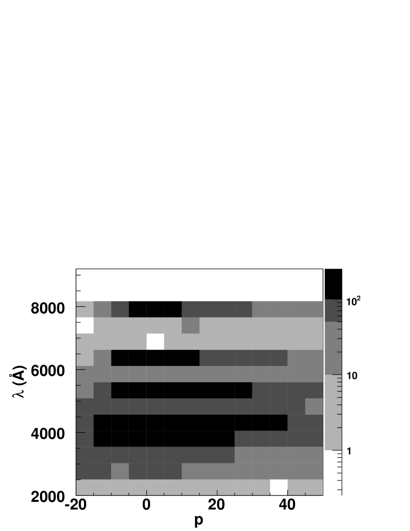
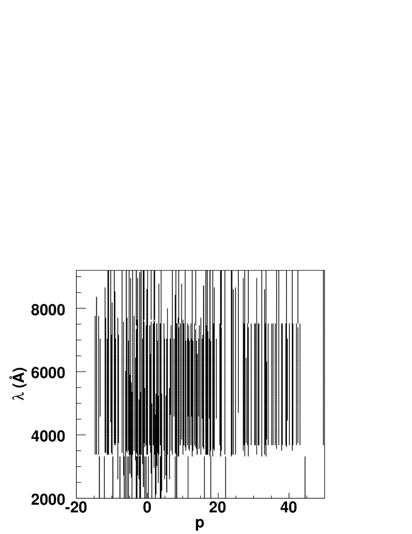
Figure 1: Phase-space mapping by photometric data (top) and spectra (bottom). For photometric observations, the rest-frame central wavelength of the filter is considered.

4 Training the model

4.1 The training procedure

The convergence process consists in minimizing a $\chi^{2}$ that permits the comparison of the full data set with the model of equation 1. For each SN, the parameters are the normalization and coordinates along the principal components $(x_{k})$, a color and re-calibration parameters for spectra if any. The actual components $(\mathbb{M}_{k})$ and the parameters of the color-law $CL(\lambda)$ also have to be estimated. This procedure requires a first guess for the model components $(\mathbb{M}_{k})$, for a first estimate of normalization, spectra re-calibration and color. We used the SALT model SED sequence for a SN with stretch $=1$ for $\mathbb{M}_{0}$ and the difference of SED sequence of a SN with stretch $=1.1$ and the previous one for $\mathbb{M}_{1}$ (i.e. a linearized version of SALT model). Additional components where initiated with the orthogonal part of the SALT model SED sequence with respect to all previous components.

We end up with more than 3000 parameters to fit, with obvious non-linearities, so that we used the Gauss-Newton procedure, which consists in:

1. Approximating locally the $\chi^{2}$ by a quadratic function of the parameters.

2. Solving a large linear system to get an increment of the parameters $(\delta P_{i})$.

3. Increment the parameters and iterate until the $\chi^{2}$ decrement with respect to the previous iteration becomes negligible.

First, the average model is estimated along with the color-law, calibration coefficients for spectra, and parameters of the SNe ( ($x_{i}$), $c$ ). When the system has converged, we add another component, and all the parameters are fitted again (components, color-law, SN parameters). The convergence algorithm is insensitive to the input set of components.

4.2 Regularization

There might be some degeneracy in part of the phase space for the given data set. For instance, if a phase$\times$wavelength region is only covered by photometry and not spectroscopy, we do not have enough data to constrain the combinations of parameters that model spectral features, whereas we can still model a photometric measurement, since the signal is integrated on a large spectral band. Adding a regularization term in the $\chi^{2}$ solves this issue. If its contribution is low enough, it will not alter significantly the determination of parameters that are addressed by the data, while putting some limitation on the parameters that are not. We have chosen to minimize second derivatives with respect to phase and wavelength (once again, effective only when there is not enough data). The regularization term is the following :

$$\chi^{2}_{REGUL}=n\times\sum{\mathbb{M}_{k}^{T}\mathbb{D}^{T}\mathbb{D}\mathbb{M}_{k}}$$

where $\mathbb{M}_{k}$ is the vector describing component $k$, $\mathbb{D}$ is the derivative matrix and $n$ a normalization that controls the weight of this regularization with respect to data. Since such a term introduces a bias in the estimator (departure from the maximum likelihood estimator), we have to quantify it in order to adjust the normalization $n$. For this purpose, we used a simulated dataset. This simulation helps us to define the resolution of the model. Each SN of the training sample was adjusted using the SALT model, then fake light-curves and spectra were computed by replacing each true measurement of the SN by the best fit value of the model. The training procedure applied to this data set gives a result that is slightly biased due to the regularization term in the $\chi^{2}$ in the UV wavelength region. The weight of the regularization term (normalization $n$) was chosen so that the bias in $K$-corrections is smaller than 0.005 mag for all wavelength, which is significantly less than the statistical uncertainties.

4.3 Model resolution

The choice of the model resolution is imposed by the data set we have. We used $10\times 120$ parameters for $\mathbb{M}_{0}$ (10 along the time axis and 120 for wavelength), in a phase range of $[-20,+50]$ days and a spectral range of $[2000,9200]\leavevmode\nobreak\ \AA$. This gives a spectral resolution of order of $60\leavevmode\nobreak\ \AA$ which is sufficient for the modeling of SNe with broad lines due to the velocity of the ejecta. For $\mathbb{M}_{1}$, we choose to use a lower resolution ( $10\times 60$ parameters). The time axis is remapped so that the time resolution at maximum and $+20$ days after maximum is a factor two better than at $-20$ and $+50$ days (approximately $4.5$ and $9$ days respectively). As in SALT, we used only two free coefficients to model the color law $CL(\lambda)$ (third order polynomial, with two coefficients fixed so that $CL(\lambda_{B})=0$ and $CL(\lambda_{V})=0.4\log(10)$, see Eq. 1). Using this number of parameters, when the model is trained with the simulated data set described above, we found that the limited resolution introduces a scatter in colors of only 0.01 mag standard deviation (it is a scatter rather than a systematic effect because of the varying epochs of photometric observations), which has a negligible on distances when compared to the intrinsic dispersion of SNe Ia luminosities.

5 Result of the training

We decided to consider only two components for the current analysis since additional components are poorly constrained in most of the phase space and marginally significant in the region of good data coverage. As the data sets improve so will the power to extract additional components. As a consequence, for each SN, we ended up with four parameters, a date of $B-$band maximum, a normalization, the parameter $x_{1}$ and a color. The average value of $x_{1}$ and its scale are arbitrary since we can modify the components in consequence. We adopted $<x_{1}>=0$ and $<x_{1}^{2}>=1$.

Figure 2 shows the variation of the UBVRI light-curves as a function of parameter $x_{1}$. We find that most of the variability can be described by a simple stretching of light-curves despite the fact that we did not force such behavior in the model. More quantitatively, the parameter $x_{1}$ can be converted into a stretch factor , whose actual value depends on the reference light-curve template used, here the one of SALT and of Goldhaber et al. (2001) ($B$-band light curve template “Parab -18”, G01); or into $\Delta m_{15}$ (Phillips, 1993) using the following transformations:

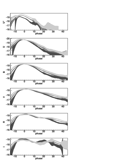
Figure 2: The $U^{*}UBVRI$ template light curves obtained after the training phase for values of $x_{1}$ of -2, 0, 2 (corresponding to stretches of 0.8, 1.0, and 1.2; dark to light curves) and null $B_{V}$ color excess. $U^{*}$ is a synthetic top hat filter in the range 2500–3500 $\AA$. The shaded areas correspond to the one standard deviation estimate as described in section 6.1.

$$s\;(SALT) =0.98+0.091x_{1}+0.003x_{1}^{2}-0.00075x_{1}^{3}$$

$$s\;(G01) =1.07+0.069x_{1}-0.015x_{1}^{2}+0.00067x_{1}^{3}$$

$$\Delta m_{15} =1.09-0.161x_{1}+0.013x_{1}^{2}-0.00130x_{1}^{3}$$

Since there is not a perfect match of the non-linear stretch and $\Delta m_{15}$ models with this one, those transformations (obtained with simulations) vary with the weight attributed to each phase (the scatter for stretch is about 0.02).

We also notice the $U-B$ color variation as a function of $B$-band light-curve broadening. The value of $U-B$ for phase=0 does not vary with $x_{1}$ (see Fig. 2), but when the flux is integrated in the phase range -10, +10 days, we find that $U-B\propto-0.2\times s(SALT)$. This is about half the value obtained with SALT. However, we find a color law very close to the one obtained with SALT (see Fig. 3), despite the fact that the supernova model is significantly different and the training set much larger.

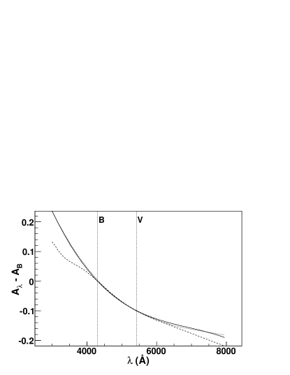
Figure 3: The color law $c\times CL(\lambda)$ as a function of wavelength for a value of $c$ of 0.1 (solid line). The dashed curve represents the extinction with respect to $B$ band, $(A_{\lambda}-A_{B})$, from Cardelli et al. (1989) with $R_{V}=3.1$ and $E(B-V)=0.1$, and the dotted line is the color law obtained with SALT (very close to the result obtained here).

These results confirm the main findings of SALT. More interesting is the variability of spectra with the first component as displayed in Figure 4 for three phases about maximum. It appears that the variability in U-band at maximum identified with light-curves can be attributed to a sharp variation of the spectrum for wavelengths lower than 3400 $\AA$. It is possible to identify such a feature thanks to the high redshift SNLS spectra. Indeed, the calibration of ground-based spectroscopic observations in the near ultraviolet may not be reliable, whereas UV spectra obtained by the International Ultraviolet Explorer have a very low signal to noise ratio for wavelengths larger than 3000 $\AA$. This feature can hardly be approximated by a broad-band color evolution. Hence we expect a net improvement of the accuracy of distance estimates in the UV range with respect to SALT or other equivalent methods which rely on a single spectral sequence. As an example of the modeling of the variability of spectral features, figure 5 presents the variation of the R(Si II), as defined in Nugent et al. (1995), as a function of $\Delta m_{15}$ retrieved from the model. It is compared to a compilation of observations by Benetti et al. (2004). There is a good match in the $\Delta m_{15}$ range of the training sample ($\Delta m_{15}<1.6$).

One must however evaluate carefully the statistical significance of the trends in the model. Statistical errors of this model rely on the weighting applied to spectra, and are sensitive to the errors assumed for photometric measurements which are not very secure for most nearby supernovae. Hence this accuracy of the modeling must be evaluated with distributions of residuals as described in the next paragraph.

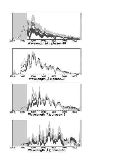
Figure 4: Spectra at -10, 0, +15 and +35 days about B-band maximum for values of $x_{1}$ of -2, 0, 2 (corresponding to stretches of 0.8, 1.0, 1.2; light gray, black curve, dark gray) and null $B_{V}$ color excess. The shaded areas correspond to the one standard deviation estimate as described in section 6.1. The dashed curves represents the spectra of N02 (version 1.2). All spectra are arbitrarily normalized.

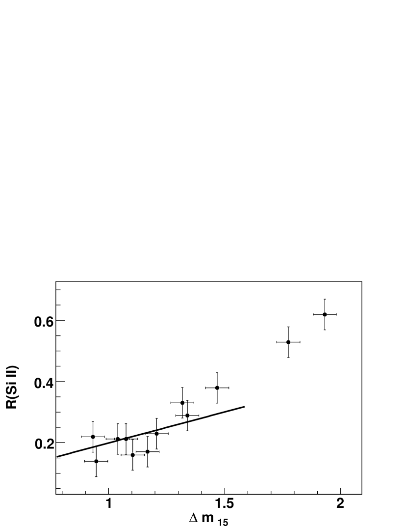
Figure 5: The solid curve presents the relation of R(Si II) (Nugent et al., 1995) as a function of $\Delta m_{15}$ along with measurements from Benetti et al. (2004).

6 The remaining variability

In order to assert the predictability of the model we need an independent data set that is not used in the training procedure. However, since we do not have a large number of measurements available, we resorted to a jackknife procedure: for each SN, we trained the model using all SNe from Table 2 but this one, and looked at residuals of the SN measurements to the retrieved model, fitting only the parameters concerning this particular SN, i.e. the date of maximum, ($x_{0,1}$), and color.

The residuals obtained by this method are a priori highly correlated, and this correlation is difficult to estimate from first principles. However we would like to use this information to extract some intrinsic variability of the SNe, beyond the principal components of the model, in order to weight data according to this variability in addition to measurement errors. We resorted to the following simplification, using two kinds of residuals (or model errors) : i) Diagonal errors of the model are estimated from fits of light-curves with an independent normalization for each of them. The residuals obtained are of course still correlated, but we allow ourselves to treat them as independent, assuming that the correlation length (along time axis) is smaller than the data sampling for most light-curves . ii) $K$-correction uncertainties, which can be estimated using the difference between the peak magnitude obtained from a single light-curve fit, and the one predicted by the model in the same filter, fitting all light-curves.

6.1 Diagonal uncertainties

We use the correlations between the estimates of the components given by the correlation matrix retrieved at the end of the training procedure. However, we allow ourself to scale these statistical uncertainties on the model in $p,\lambda$ bins to account for the remaining variability.

The model variance can then be defined as :

$$V_{MODEL}(x_{1},p,\lambda) = S(p,\lambda)\times V_{MEAN}(x_{1},p,\lambda)$$

$$V_{MEAN}(x_{1},p,\lambda) = \mathbb{H}_{0}^{T}\mathbb{V}_{0}\mathbb{H}_{0}+x_{1}^{2}\mathbb{H}_{1}^{T}\mathbb{V}_{1}\mathbb{H}_{1}+2x_{1}\mathbb{H}_{0}^{T}\mathbb{C}_{0,1}\mathbb{H}_{1}$$

where $\mathbb{H}_{0}(p,\lambda)$ and $\mathbb{H}_{1}(p,\lambda)$ are the vectors defined in Sec. 2.1 for components 0 and 1, $\mathbb{V}_{0}$, $\mathbb{V}_{1}$ and $\mathbb{C}_{0,1}$ are the full variance and covariance matrices of the components, and $S(p,\lambda)$ the scaling function.

In each $p,\lambda$ bin, $S(p,\lambda)$ is evaluated so that

$$\frac{1}{n}\sum\frac{\left[f_{i}-x_{0}\left(\mathbb{H}_{0,i}^{T}\mathbb{M}_{0}+x_{1}\mathbb{H}_{0,i}^{T}\mathbb{M}_{1}\right)\right]^{2}}{\sigma_{i}^{2}+x_{0}^{2}S(p,\lambda)V_{MEAN}(x_{1},p,\lambda)}=1$$

where $(f_{i})$ and $(\sigma_{i})$ are the measurements and their associated uncertainties. We evaluated separately these errors for light-curves and spectra, in order to take into account the correlated errors along the wavelength axis when dealing with photometric data.

Photometric residuals of the jackknife-like procedure are shown figure 6. The data set are split in four rest-frame wavelength ranges, $[3200,3900]$, $[3900,5000]$, $[5000,5700]$ and $[5700,7300]$ $\AA$, that roughly correspond to U, B, V, R and I bands respectively. The model uncertainties basically follow the statistical errors of data, with very good accuracy at peak brightness and a poor quality at early and late phases, especially in the $U-$band. In the rise time region, the large errors are partly due to the limiting resolution of the model. Those errors are also displayed in figure 2 for $|x_{1}|$=2.

When fitting spectra, we imposed the values of the date of maximum, $x_{1}$ and color obtained with the light-curves fit. The only remaining free parameters were those used to photometrically ”re-calibrate” spectra. We found that model accuracy is poor at early phases and in the UV region (Fig. 4).

These estimates of the model errors can be accounted for when fitting the light-curves or spectra. It gives more reliable statistical errors for parameters (peak brightness, color, $x_{1}$ and date of maximum) than when only statistical errors of measurements are considered.

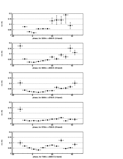
Figure 6: Estimated standard deviation of model photometric errors as a function of phase, for several rest-frame wavelength ranges roughly corresponding from top to bottom to $U$, $B$, $V$, $R$ and $I-$bands. Those model errors were evaluated from the scatter of residuals to the single light-curve fit.

6.2 $K$-correction uncertainties

A direct approach to access the quality of $K$-corrections is to compare the observed peak magnitude of a light-curve in a given filter with the one predicted by the model using a fit of the other light-curves. Figure 7 presents the differences between the observed and predicted magnitudes as a function of the effective rest-frame wavelength of the instrument response used.

A more elaborated approach consists in modeling $K$-correction errors with a parametric function of wavelength which value vanishes for wavelength corresponding to the rest-frame $B$ and $V-$bands (errors on $B$ and $V$ magnitudes at maximum enter in the normalization and color evaluation). For each SN with enough light-curves, those $K$-correction additional parameters can be estimated and their standard deviation used to derive a model of $K$-correction errors. Such a model is represented by the solid line figure 7 and is given by the following formula:

$$\sigma_{K}(\lambda)= 0.022\left(\frac{\lambda-\lambda_{B}}{\lambda_{U}-\lambda_{B}}\right)^{3} \mathrm{for}\,\lambda<\lambda_{B}$$

$$= 0.018\left(\frac{\lambda-\lambda_{V}}{\lambda_{R}-\lambda_{V}}\right)^{2} \mathrm{for}\,\lambda>\lambda_{V}$$

Since the estimate of $\sigma_{K}$ is based on the fit of the normalization of light-curves, it measures a dispersion of colors averaged over the phase range defined by the data set. Clearly, the $K$-correction errors are large in the UV range. Also, those errors must be added to the statistical errors on normalizations, but they do not account for the whole observed scatter. For instance, for $\lambda_{U}\simeq 3600\AA$, we find a dispersion of 0.04 magnitude (consistent with the one obtained in A06, Fig. 11.), but an uncertainty of only 0.022 magnitude has to be added to the statistical errors to match the observed dispersion. Diagonal uncertainties and $K$-correction uncertainties are taken into account in the fits performed in the following section.

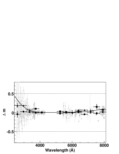
Figure 7: Difference between observed peak magnitude in each band of each SN from table 2 and the model prediction as a function of the rest-frame effective wavelength of the filter used (gray triangles : SNLS SNe, gray squares : nearby SNe). The large black symbols represent the estimated dispersion in each wavelength bin (triangles for SNLS, and squares for nearby SNe). The large circles show the average difference in each wavelength bin for all SNe and the solid curve is a polynomial fit to the dispersion used as an estimate of the $K$-correction scatter. Since uncertainties on $B$ and $V$ magnitudes at maximum enter in the normalization and color evaluation of the model, $K$-correction uncertainties are set to zero for $B$ and $V-$ band wavelengths.

7 Improving the distance estimates of distant SNe

Despite the fact that our modeling is less accurate in the UV range, it is still very useful for distance estimates of high-redshift SNe ($z>0.8$) for which, as in the case of SNLS, the rest-frame $B$ and $V$-band observations often have a very poor signal to noise ratio.

7.1 Light-curve fit of distant supernovae

Figure 8 shows the SN Ia SNLS-04D3gx at $z=0.91$ fitted by the model. All four light-curves (g,r,i,z) are well described by the best fit model for which only four parameters were adjusted (date of maximum, normalization, color and $x_{1}$). The $\chi^{2}$ per degree of freedom (d.o.f.) of the fit is 0.76 (for 50 d.o.f.) when diagonal and $K$-correction uncertainties of the model are considered. Table 1 illustrates the gain in the accuracy of the color estimate for SNLS-04D3gx.

bands	$\lambda_{\mathrm{min}}$	color
i,z	3980	$-0.220\pm 0.180\mathrm{(s)}\pm 0.033\mathrm{(d)}\pm 0.005\mathrm{(k)}$
r,i,z	3250	$-0.147\pm 0.051\mathrm{(s)}\pm 0.026\mathrm{(d)}\pm 0.049\mathrm{(k)}$
g,r,i,z	2520	$-0.172\pm 0.047\mathrm{(s)}\pm 0.023\mathrm{(d)}\pm 0.047\mathrm{(k)}$

Table 1: Error on the color estimate of SNLS-04D3gx as a function of the number of light-curves included in the fit. The contributions to the error are measurement statistical errors (s), diagonal model errors (d) and $K$-correction errors (k).

The total uncertainty on the color parameter is reduced by a factor 2.5 when g and r-band (rest-frame UV) light-curves are included in the fit. We see that the model uncertainties are large in this wavelength range and therefore must be propagated.

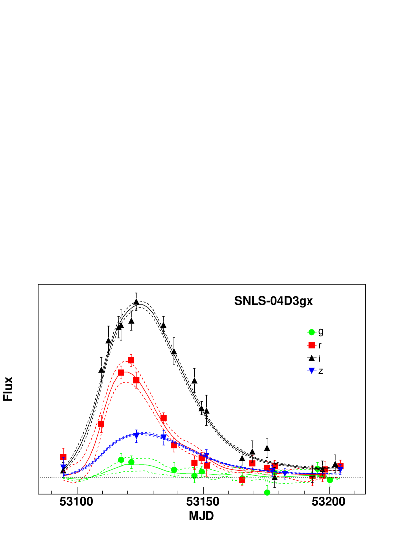
Figure 8: Observed light-curves points of the SN Ia SNLS-04D3gx at z=0.91 along with the light-curves derived from the model (solid line, trained without this SN). The dashed lines represent the 1 $\sigma$ uncertainties of the model (both uncorrelated and $K$-correction errors).

7.2 Improving cosmological results

The parameters retrieved from the light-curve fit can be used to estimate distances using the same procedure as described in A06. The distance estimator is a linear combination of $m^{*}_{B},x_{1}$ and $c$ :

$$\mu_{B}=m^{*}_{B}-M+\alpha_{x}\times x_{1}-\beta\times c$$

with $m^{*}_{B}$, $x_{1}$ and $c$ derived from the fit to the light curves, and $\alpha_{x}$ , $\beta$ and the absolute magnitude $M$ are parameters which are fitted by minimizing the residuals in the Hubble diagram. As in A06, we introduce an additional ”intrinsic” dispersion ($\sigma_{int}$) of SN absolute magnitudes to obtain a reduced $\chi^{2}$ of unity for the best fit set of parameters.

We minimize the following functional form, which gives negligible biases to the estimates of $\alpha_{x}$ and $\beta$:

$$\chi^{2}=\sum_{s}\frac{{\bf V}^{T}{\bf X}_{s}-M-5\log_{10}\left(d_{L}({\bf\theta},z)/10\,\mathrm{pc}\right)}{\bf{V}^{T}\;{\bf C}({\bf X}_{s})\;{\bf V}}$$

with

$${\bf X}_{s}=\begin{pmatrix}m^{*}_{B}\\ x_{1}\\ c\\ \end{pmatrix},\,\,{\bf V}=\begin{pmatrix}1\\ \alpha_{x}\\ -\beta\\ \end{pmatrix}$$

${\bf\theta}$ stands for the cosmological parameters that define the fitted model and $d_{L}$ is the luminosity distance. ${\bf C}({\bf X}_{s})$ is the covariance matrix of the parameters ${\bf X}_{s}$ for which we have included in the variance of $m^{*}_{B}$ the intrinsic dispersion and an error of the distance modulus due to peculiar velocities, which we take to be 300 km.s^-1.

To estimate the systematic effect due to modeling of the SN Ia SED sequence, we fit the data set of A06, which consists in 44 nearby SNe Ia and 71 SNLS SNe. Whereas we used improved photometry for the training of the model, we consider here exactly the same data set as in A06, in order to ease the comparison with the results obtained with SALT.

Thanks to the evaluation of the model errors, we can safely use all available light-curves in the fit. Especially the $r-$band data at redshifts greater than 0.8 (effective rest-frame wavelength lower than 3440 $\AA$) are very useful to constrain the color of the supernova. With this additional information, the uncertainty in distance moduli is significantly reduced at high redshift, yielding a better resolution on cosmological parameters. For flat $\Lambda$CDM cosmology, we obtain :

$$\Omega_{M} = 0.240\pm 0.033$$

$$\alpha_{x} = 0.13\pm 0.013$$

$$\beta = 1.77\pm 0.16$$

with $\sigma_{int}=0.12$ (which is smaller than the value of 0.13 in A06 because we have considered uncertainties in the model). The RMS of the residuals around the best fit Hubble relation is 0.161 mag (compared to 0.20 in A06, see Fig. 9).

The uncertainty on $\Omega_{M}$ is improved by 10% with respect to the A06 ($\Omega_{M}=0.263\pm 0.037$, table 3 of Astier et al. 2006) analysis. We find a difference of 0.023 on $\Omega_{M}$ which is consistent with the assumed systematic error due to modeling of 0.02 in that paper. However the supernova SNLS-03D1cm at a redshift of 0.87 now appears as a significant outlier as the distance modulus resolution improved . This object has a spectrum with low signal to noise ratio and was classified as probable Ia. Discarding this object from the analysis gives $\Omega_{M}=0.246\pm 0.032$ and a standard deviation of residuals of 0.154 magnitude.

Since the current model significantly improves distance estimates at high redshifts, we obtain a greater improvement on the estimation of the equation of state of dark energy. As an example, we may use the figure of merit proposed by the Dark Energy Task Force (Albrecht et al., 2006), which is inversely proportional to the area of the 95% confidence level contour in the plane $(w_{a},w_{p})$, where the following parametrization is considered for the equation of state of dark energy :

$$w=w_{p}+(a_{p}-a)w_{a}$$

$a$ being the scale factor, and $a_{p}$ a reference scale factor chosen so that the estimates of $w_{p}$ and $w_{a}$ are uncorrelated for a given experiment. Using the baryon acoustic oscillations constraints from Eisenstein et al. (2005) (Eq. 4), $a_{p}=0.851$, and we improve this figure of merit by 35% with respect to the analysis using SALT (for which $a_{p}$ is slightly different).

Light-curves can be fitted with all the models from the jackknife procedure, so that we can derive as many estimates of $\Omega_{M}$ as there are SNe in the training sample. We found that the RMS of this distribution is 0.003, so that we expect a deviation from a model trained with an infinite number of SNe of the order of 0.0015 on $\Omega_{M}$ (for a flat $\Lambda$CDM cosmology), a value that is negligible compared to the other sources of systematic errors in such an analysis.

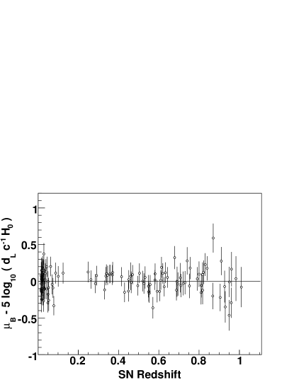
Figure 9: Residuals to the distance redshift relation for the best fit $\Lambda$CDM cosmology for SNLS and nearby SNe Ia.

8 Other applications

The proposed model provides a tool for spectroscopic and photometric identification, and photometric redshift determination. A detailed analysis of the purity and efficiency of a photometric identification tool with respect to SNe Ib, Ic and II is beyond the scope of this paper.

8.1 Spectroscopic identification

The model proposed allows simultaneous fits of light-curves and spectra (with additional galaxy templates to evaluate the host contamination as mentioned in Sec. 3.2). This can turn out to be very useful for identification of Type Ia supernovae. Indeed, some Type Ic SNe can present light-curves and spectra that look qualitatively like SNe Ia, and in the most extreme cases, photometric and spectroscopic identifications taken separately may fail to tag this object correctly. A detailed analysis is beyond the scope of this paper. We will show only two examples.

First, figure 10 shows the observed light-curves and spectrum of SNLS-03D4ag at a redshift of 0.285 along with the result of the simultaneous fit. Four “re-calibration” parameters for the spectrum were considered (since there are four light-curves). The $\chi^{2}$ per degree of freedom for the light-curves and the spectrum are respectively 0.53 (for 28 d.o.f.) and 0.63 (for 1770 d.o.f.), taking into account the model errors ), so that this SN can be safely considered as a typical normal SN Ia.

Figure 10: Top: Observed light-curves points of the SN Ia SNLS-03D4ag at z=0.285 along with the light-curves derived from the model (solid line). Bottom: Observed VLT spectrum at a phase of -8 days along with the model spectrum. The dashed curve is the expected model from the light-curve fit (up to a global normalization) and the solid curve the one including four re-calibration parameters.

Now if we consider an SN Ic, for instance SNLS-03D4aa at a redshift of 0.166, the model gives a very bad fit of the data (reduced $\chi^{2}$ of 4.6 (for 10 d.o.f.) and 1.6 (for 1807 d.o.f) for light-curves and spectra respectively), allowing for a clear rejection of this event.

8.2 Photometric redshifts

For photometric redshift determination, one can compare the redshift estimate based on a simultaneous fit of all light-curves of a given supernova and the much more precise spectroscopic redshift derived from the spectroscopic observation of the host of the object. Using all available light-curves (up to four for SNLS) allows us to relax assumptions on the light curve shape parameter ($x_{1}$) and the color, without any use of the absolute luminosity, so that we do not require any prior on the cosmological parameters.

We have applied this method to all SNe Ia from Table 2 with at least 3 light-curves, using for each SN the model obtained without this SN (always to avoid over-training). A Gaussian prior for $x_{1}$ was assumed based on the statistics from the training procedure, $x_{1}=0\pm 1$. No prior was applied to color.

The resulting photometric redshift is compared to the spectroscopic one on Figure 11. The RMS of the distribution of $\Delta z/(1+z)$ is 0.02 with no significant bias. A Gaussian fit of the distribution of $\Delta z/(1+z)$ gives $\sigma=0.01$. This is an accuracy of the same order of magnitude as the one that can be derived from a fit of the SN spectrum alone. The only low-redshift SN for which the photometric redshift is off by more than 0.1 is SN1999cl which is a highly extincted supernova.

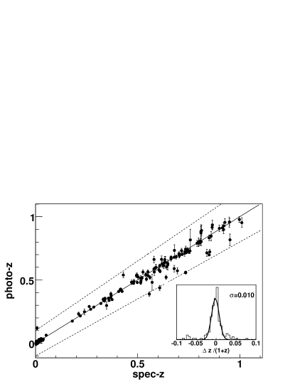
Figure 11: Photometric vs spectroscopic redshifts for the training sample of SNe. The dashed lines are $z\pm 0.1(1+z)$ functions.

9 Conclusion

We have proposed a new empirical model of Type Ia supernovae spectro-photometric evolution with time, based on observed nearby and distant supernovae light-curves and spectra. The method uses available spectra, regardless of their wavelength range or calibration accuracy, since they are re-calibrated using the photometric information in the training process. This model provides an average spectral sequence of Type Ia supernovae and their principal variability components .

Thanks to an evaluation of the modeling errors (for photometric points, spectra, and broad-band colors), on can safely use most of the information on a given supernova for comparison with the model. This is very helpful for distance estimates, but also photometric redshift evaluation and SN identification.

Applied to the supernovae sample of A06, we improved the distance estimates, especially at redshifts larger than 0.8, thanks to the modeling of the ultraviolet emission and the propagation of model errors. When a flat $\Lambda$CDM cosmology is fitted to the Hubble diagram, the gain in statistical resolution on $\Omega_{M}$ is of 10% compared to the previous analysis using SALT; it is 35% better on the two parameter constraint of the equation of state of dark energy.

The model accuracy is currently limited by the size and quality of the current data sample. A larger sample would be needed to look for another variability component.

This empirical modeling technique is well suited for the analysis of very large samples of supernovae photometric data such as the ones expected from future projects like DUNE (Réfrégier et al., 2006), JDEM (Aldering, 2004) or LSST . Indeed, with large statistics of high precision photometric data spread on a large redshift range, we may expect to deconvolve the SED sequence of the average supernova and its principal variations. Such an analysis would permit one to look for variability correlated with redshift, and hence provide a non-parametric approach to test for supernova evolution.

Table 2: The training sample of Type Ia supernovae light curves and spectra

Name	$z$	Bands	Number of spectra; phases
1981B	0.006	UBV (B83)	6 ;   $0\leq p\leq 35$ (Br83)
1986G	0.002	BV (P87)	6 ;   $-3\leq p\leq 18$ (AC)
1989B	0.002	UBVR (W94)	18 ;   $-6\leq p\leq 19$ (AC)
1990af	0.051	BV (H96)	0
1990N	0.003	UBVR (L91,L98)	15 ;   $-14\leq p\leq 38$ (AC,IUE,CFA)
1991T	0.006	UBVR (F92,L98,A04,K04b)	36 ;   $-13\leq p\leq 258$ (AC,CFA)
1992A	0.006	UBVR (S92,A04)	19 ;   $-5\leq p\leq 27$ (CFA,IUE)
1992al	0.015	BVR (H96)	0
1992bc	0.020	BVR (H96)	0
1992bo	0.019	BVR (H96)	0
1993O	0.052	BV (H96)	0
1994ae	0.004	BVR (R99,A04)	0
1994D	0.001	UBVR (R95,P96,M96,A04)	21 ;   $-11\leq p\leq 76$ (AC)
1994S	0.015	BVR (R99)	1 ;   $p=22$ (AC)
1995ac	0.050	BVR (R99)	0
1995al	0.005	BVR (R99)	0
1995bd	0.016	BVR (R99)	0
1995D	0.007	BVR (R99,A04)	0
1995E	0.012	BVR (R99)	0
1996bl	0.036	BVR (R99)	0
1996bo	0.017	UBVR (R99,A04)	0
1996X	0.007	BVR (R99)	12 ;   $-1\leq p\leq 57$ (AC)
1997bp	0.008	UBVR (J05)	0
1997bq	0.009	UBVR (J05)	0
1997do	0.010	UBVR (J05)	0
1997E	0.013	UBVR (J05)	0
1998ab	0.027	UBVR (J05)	0
1998aq	0.004	UBVR (R05)	26 ;   $-9\leq p\leq 90$ (CFA)
1998bu	0.003	UBVR (S99)	66 ;   $-3\leq p\leq 56$ (CFA)
1998dh	0.009	UBVR (J05)	0
1998ef	0.018	UBVR (J05)	0
1998es	0.011	UBVR (J05)	0
1999aa	0.014	UBVR (J05)	9 ;   $-11\leq p\leq 40$ (G04)
1999ac	0.009	UBVR (J05)	0
1999aw	0.038	BVR (St02)	0
1999cl	0.008	UBVR (J05,K00)	0
1999dk	0.015	UBVR (K01,A04)	0
1999dq	0.014	UBVR (J05)	0
1999ee	0.011	UBVR (S02)	11 ;   $0\leq p\leq 43$ (H02)
1999ek	0.018	UBVR (J05,K04b)	0
1999gp	0.027	UBVR (J05,K01)	0
2000E	0.005	UBVR (V03)	0
2000fa	0.021	UBVR (J05)	0
2001ba	0.029	BV (K04a)	0
2001bt	0.014	BVR (K04b)	0
2001cz	0.016	UBVR (K04b)	0
2001el	0.004	UBVR (K03)	2 ;   $p=24,33$ (W03)
2001V	0.015	BVR (Vi03)	0
2002bo	0.004	UBVR (Z03,B04,K04b)	12 ;   $-14\leq p\leq 38$ (B04)
2002er	0.009	UBVR (P04)	0
2003du	0.006	UBVR (A05)	4 ;   $-11\leq p\leq 37$ (A05)
2004fu	0.009	UBVR (T06)	0
SNLS-03D1au	0.504	griz	0
SNLS-03D1aw	0.582	griz	0
SNLS-03D1ax	0.496	griz	1 ;   $p=-3$
SNLS-03D1bk	0.865	griz	1 ;   $p=-6$
SNLS-03D1co	0.679	griz	1 ;   $p=-4$
SNLS-03D1ew	0.868	griz	1 ;   $p=1$
SNLS-03D1fc	0.331	griz	1 ;   $p=-3$
SNLS-03D1fl	0.688	griz	1 ;   $p=1$
SNLS-03D1fq	0.800	griz	0
SNLS-03D4ag	0.285	griz	1 ;   $p=-8$
SNLS-03D4at	0.633	griz	1 ;   $p=6$
SNLS-03D4cj	0.270	griz	1 ;   $p=-9$
SNLS-03D4cx	0.949	griz	0
SNLS-03D4cy	0.927	griz	0
SNLS-03D4cz	0.695	griz	0
SNLS-03D4dh	0.627	griz	0
SNLS-03D4dy	0.604	griz	1 ;   $p=4$
SNLS-03D4fd	0.791	griz	1 ;   $p=-1$
SNLS-03D4gl	0.571	griz	0
SNLS-04D1ag	0.557	griz	1 ;   $p=4$
SNLS-04D1dc	0.211	griz	1 ;   $p=-1$
SNLS-04D1ff	0.860	griz	1 ;   $p=4$
SNLS-04D1hd	0.369	griz	1 ;   $p=0$
SNLS-04D1hx	0.560	griz	1 ;   $p=5$
SNLS-04D1hy	0.850	griz	1 ;   $p=-2$
SNLS-04D1iv	0.998	griz	1 ;   $p=2$
SNLS-04D1kj	0.584	griz	1 ;   $p=-4$
SNLS-04D1ks	0.798	griz	1 ;   $p=-1$
SNLS-04D1oh	0.590	griz	0
SNLS-04D1ow	0.915	griz	1 ;   $p=5$
SNLS-04D1pc	0.758	griz	0
SNLS-04D1pd	0.952	griz	0
SNLS-04D1pg	0.515	griz	1 ;   $p=-1$
SNLS-04D1pp	0.735	griz	0
SNLS-04D1sa	0.589	griz	1 ;   $p=-2$
SNLS-04D1si	0.704	griz	0
SNLS-04D1sk	0.663	griz	0
SNLS-04D2ac	0.348	griz	0
SNLS-04D2cf	0.369	griz	1 ;   $p=8$
SNLS-04D2fp	0.415	griz	1 ;   $p=1$
SNLS-04D2fs	0.357	griz	1 ;   $p=1$
SNLS-04D2gb	0.430	griz	0
SNLS-04D2gc	0.521	griz	1 ;   $p=-4$
SNLS-04D2gp	0.707	griz	1 ;   $p=2$
SNLS-04D2kr	0.744	griz	0
SNLS-04D3co	0.620	griz	0
SNLS-04D3dd	1.010	griz	1 ;   $p=2$
SNLS-04D3df	0.470	griz	0
SNLS-04D3do	0.610	griz	0
SNLS-04D3ez	0.263	griz	0
SNLS-04D3fk	0.358	griz	0
SNLS-04D3fq	0.730	griz	1 ;   $p=1$
SNLS-04D3hn	0.552	griz	0
SNLS-04D3kr	0.337	griz	1 ;   $p=4$
SNLS-04D3mk	0.813	griz	0
SNLS-04D3ml	0.950	griz	0
SNLS-04D3nh	0.340	griz	1 ;   $p=3$
SNLS-04D3ny	0.810	griz	1 ;   $p=1$
SNLS-04D3oe	0.756	griz	0
SNLS-04D4an	0.613	griz	0
SNLS-04D4bq	0.550	griz	2 ;   $p=2,4$
SNLS-04D4dm	0.811	griz	0
SNLS-04D4fx	0.629	griz	1 ;   $p=-8$
SNLS-04D4gg	0.424	griz	0
SNLS-04D4hu	0.703	griz	0
SNLS-04D4ic	0.680	griz	1 ;   $p=2$
SNLS-04D4ii	0.866	griz	0
SNLS-04D4im	0.751	griz	0
SNLS-04D4in	0.516	griz	0
SNLS-04D4jr	0.482	griz	1 ;   $p=-6$
SNLS-05D1ck	0.617	griz	0
SNLS-05D2ab	0.320	griz	0
SNLS-05D2ac	0.494	griz	0
SNLS-05D2ah	0.180	griz	0
SNLS-05D2ay	0.921	griz	0
SNLS-05D2bt	0.679	griz	0
SNLS-05D2bv	0.474	griz	0
SNLS-05D2bw	0.921	griz	0
SNLS-05D2ci	0.631	griz	0
SNLS-05D2cl	0.839	griz	0
SNLS-05D2ct	0.734	griz	0
SNLS-05D2dw	0.417	griz	0
SNLS-05D2dy	0.498	griz	0
SNLS-05D2eb	0.639	griz	0
SNLS-05D2ec	0.526	griz	0
SNLS-05D2fq	0.735	griz	0
SNLS-05D2hc	0.360	griz	0
SNLS-05D2he	0.608	griz	0
SNLS-05D3ax	0.643	griz	0
SNLS-05D3cf	0.419	griz	0
SNLS-05D3ci	0.515	griz	0
SNLS-05D3cx	0.805	griz	0
SNLS-05D3dd	0.480	griz	0
SNLS-05D3gp	0.580	griz	0
SNLS-05D3gv	0.715	griz	0
SNLS-05D3ha	0.808	griz	0
SNLS-05D3hq	0.338	griz	0
SNLS-05D3hs	0.664	griz	0
SNLS-05D3ht	0.900	griz	0
SNLS-05D3jb	0.740	griz	0
SNLS-05D3jh	0.718	griz	0
SNLS-05D3jk	0.736	griz	0
SNLS-05D3jq	0.579	griz	0
SNLS-05D3jr	0.370	griz	0
SNLS-05D3kp	0.850	griz	0
SNLS-05D3kt	0.648	griz	0
SNLS-05D3kx	0.219	griz	0
SNLS-05D3lb	0.647	griz	1 ;   $p=-1$
SNLS-05D3mq	0.240	griz	0
SNLS-05D4af	0.502	griz	0
SNLS-05D4ag	0.636	griz	0
SNLS-05D4av	0.543	griz	0
SNLS-05D4be	0.540	griz	0
SNLS-05D4bj	0.704	griz	0
SNLS-05D4ca	0.608	griz	0
SNLS-05D4cq	0.783	griz	0
SNLS-05D4cs	0.735	griz	0
SNLS-05D4cw	0.375	griz	0
SNLS-05D4dt	0.407	griz	0
SNLS-05D4dw	0.853	griz	0
SNLS-05D4dy	0.810	griz	0