Kinematics and Chemistry of the Hot Molecular Core in G34.26+0.15 at High Resolution

Abstract

We present high angular resolution ($\sim 1$″) multi-tracer spectral line observations toward the hot core associated with G34.26+0.15 between 87–109 GHz. We have mapped emission from (i) complex nitrogen- and oxygen-rich molecules like CH₃OH, HC₃N, CH₃CH₂CN, NH₂CHO, CH₃OCH₃, HCOOCH₃; (ii) sulfur-bearing molecules like OCS, SO and SO₂; and (iii) the recombination line H53$\beta$.

The high angular resolution enables us to directly probe the hot molecular core associated with G34.26+0.15 at spatial scales of 0.018 pc. At this resolution we find no evidence for the hot core being internally heated. The continuum peak detected at $\lambda=2.8$ mm is consistent with the free-free emission from component C of the ultracompact H ii region. Velocity structure and morphology outlined by the different tracers suggest that the hot core is primarily energized by component C. Emission from the N- and O-bearing molecules peak at different positions within the innermost regions of the core; none are coincident with the continuum peak. Lack of high resolution complementary datasets makes it difficult to understand whether the different peaks correspond to separate hot cores, which are not resolved by the present data, or manifestations of the temperature and density structure within a single core.

Based on the brightness temperatures of optically thick lines in our sample, we estimate the kinetic temperature of the inner regions of the HMC to be $160\pm 30$ K. Comparison of the observed abundances of the different species in G34.26+0.15 with existing models does not produce a consistent picture. There are uncertainties due to: (i) the unavailability of temperature and density distribution of the mapped region within the hot core, (ii) typical assumption of centrally peaked temperature distribution for a hot core with an accreting protostar at the center, by the chemical models, an aspect not applicable to externally heated hot cores like G34.26+0.15 and (iii) inadequate knowledge about the formation mechanism of many of the complex molecules.

1 Introduction

Hot cores are compact (0.1 pc), warm ($\sim$ 100–300 K), dense (10⁷ H nuclei cm^-3) clouds of gas and dust near or around sites of recent star formation (see e.g. Kurtz et al., 2000; Cesaroni, 2005; van der Tak, 2005). The hot-core phase is thought to last about 10⁵ yr (van Dishoeck & Blake, 1998) to 10⁶ yr (Garrod & Herbst, 2006) and represents the most chemically rich phase of the interstellar medium, characterized by complex molecules like CH₃OH, CH₃CN, HCOOCH₃, CH₃OCH₃ and CH₃CH₂CN. The complex chemical and physical processes occurring in the hot-cores are not fully understood. Until recently hot cores were thought to be associated with high-mass protostars (M$\geq$ 8 $\mathrm{M}_{\odot}$) only and to represent an important phase in their evolution toward ultracompact and compact H ii regions. The central energizing source for a number of hot cores have been identified using high angular resolution mid-infrared (MIR) and millimeter continuum observations (e.g. De Buizer et al., 2003; Beltrán et al., 2004). These detections strengthen the idea of hot molecular cores (HMCs) as representing a stage in the evolutionary sequence of massive protostars. However, there are non-negligible examples of hot cores that are in the vicinities of UC H ii regions and appear to be only externally heated. For these sources it may well be argued that the hot cores can also arise as chemical manifestations of the effect of the UC H ii regions on their environments, rather than being only the precursors of UC H ii regions.

The chemical models are still far from providing a unique interpretation of the hot core chemistry, and would benefit from high angular resolution continuum and spectroscopic observations suitable to understand the temperature and density distributions of the cores. In particular, the strong sensitivity of surface and gas-phase chemistry to dust temperature and gas density highlights the importance of the study of the abundances of complex molecules in different regions with varied physical characteristics. Furthermore, all the existing chemical models assume the hot cores to be internally heated and have radially varying density and temperature profiles (Millar et al., 1997; Nomura & Millar, 2004; Garrod & Herbst, 2006; Doty et al., 2006); the models do not yet provide a consistent treatment of the externally heated hot cores.

We present high angular resolution (1″) interferometric observations with the Berkeley-Illinois-Maryland Association (BIMA) array of the well-studied hot core associated with the UC H ii region G34.26+0.15 located at a distance of 3.7 kpc (Kuchar & Bania, 1994). The H ii region is a prototypical example of cometary morphology, which may be due to the bow-shock interaction between an ambient molecular cloud and the wind from an energetic young star moving supersonically through the cloud (Wood & Churchwell, 1989; van Buren et al., 1990). NH₃ observations with the VLA (Heaton et al., 1989) show that the highly compact molecular cloud appears to be wrapped around the head of the cometary H ii structure, with the ionization front advancing into the cloud.

G34.26+0.15 has been extensively studied in radio continuum (Turner et al., 1974; Reid & Ho, 1985; Wood & Churchwell, 1989) and radio recombination lines (Garay et al., 1985, 1986; Gaume et al., 1994; Sewilo et al., 2004). At radio continuum frequencies, it exhibits several components: two UC H ii regions called A & B, a more evolved H ii region with a cometary shape named component C, and an extended ring-like H ii region with a diameter of 1′ called component D (Reid & Ho, 1985). Molecular gas has been mapped in NH₃, HCO⁺, SO, CH₃CN and CO (Henkel et al., 1987; Heaton et al., 1989; Carral & Welch, 1992; Heaton et al., 1993; Akeson & Carlstrom, 1996; Watt & Mundy, 1999).

The hot core associated with G34.26+0.16 has been the target of chemical surveys using single-dish telescopes (MacDonald et al., 1996; Hatchell et al., 1998) in which complex molecules characteristic of hot cores were detected. Molecular line observations suggest that the hot core does not coincide with the H ii region component C; it is offset to the east by at least 2″ and shows no sign of being internally heated (Heaton et al., 1989; MacDonald et al., 1995; Watt & Mundy, 1999). Based on narrow-band mid-infrared imaging of the complex, Campbell et al. (2000) concluded that the same star is responsible for the ionization of the H ii component C and heating the dust but is not interacting with the hot core seen in molecular emission. At a resolution of 12″, Hunter et al. (1998) also found the peak of the 350 µm emission to be coincident with the component C of the UC H ii region.

In this paper we use the BIMA observations to study the energetics, chemistry and kinematics of the molecular gas contributing to the hot core emission associated with G34.26+0.15.

2 Observations

Observations of the source G34.26+0.15 were acquired with the ten-element BIMA interferometer between 1999 December and March 2000 at three frequency bands centered approximately at 87, 107 and 109 GHz using the A & B configurations of the array. Due to technical difficulties only nine antennas could be used for the observations at 87 GHz. Table 1 presents a log of the observations, including the typical system temperatures in the different configurations presented here. The primary FWHM of the array is between 132″ and 106″ at frequencies between 87 and 109 GHz. The correlator was configured to split each frequency into four windows per sideband, two of which had bandwidths of 100 MHz and 64 channels each and the remaining two had bandwidths of 50 MHz and 128 channels each.

The sources Uranus, 1830+063 and 1771+096 were observed as the primary flux calibrator, the phase calibrator and the secondary calibrator, respectively. However owing to the consistently poor quality of 1830+063 observations and the sparsity of Uranus observations, we have used 1771+096 as both the phase and primary flux calibrator. The flux of 1771+096 was determined from each of the six datasets, using the MIRIAD task bootflux with Uranus as the primary calibrator. The average final flux for 1771+096 is 2.3 Jy; we estimate the absolute flux calibration error to be 10%. The pointing and phase center used for mapping the region around G34.26+0.15 is $\alpha_{2000}$ = 18^h53^m18$\fs$55 $\delta_{2000}$ = 1°14′58$\farcs$2 and the $V_{\rm lsr}$ = 58 km s^-1.

The data were reduced using the MIRIAD (Sault et al., 1995) software package. Continuum maps were constructed by averaging over spectral windows that did not contain line emission. In order to achieve better phases the continuum maps were iteratively self calibrated. The spectral line maps within a particular spectral window were made by first fitting a low-order polynomial to the visibilities in the channels not contaminated by any line emission and then subtracting the fit to the continuum from the individual channels.

3 Results

3.1 Spectral Lines

The observed spectral lines were identified using the spectral line catalog by Lovas et al. (1979). We have detected multiple transitions of methanol (CH₃OH), two transitions of ethyl cyanide (CH₃CH₂CN) and single transitions of methyl formate (HCOOCH₃), dimethyl ether (CH₃OCH₃), formamide (NH₂CHO), HC₃N, OCS (and its ³⁴S, ¹³C isotopomers), SO, SO₂ and the hydrogen recombination line H53$\beta$. Table 2 presents spectroscopic details of the molecular lines that were detected in the present data set.

Table 3 summarizes the basic results of the BIMA observations: synthesized beam sizes, the peak intensity, the peak brightness temperature, the central velocity ($v_{\rm cen}$), the velocity width ($v_{\rm fwhm}$) and the achieved rms per channel of the interferometric maps, for each of the observed spectral lines. The $v_{\rm cen}$ and $v_{\rm fwhm}$ were determined from Gaussian fits to the line profiles. In addition to the 10% error in absolute calibration we estimate the statistical errors in intensities to be $\sim 10$%.

3.2 Continuum at $\lambda=2.8$ mm

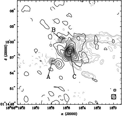
Figure 1: Overlay of the contours (black) of the 2.8 mm continuum emission detected with BIMA with the contours (grey) of the 2 cm free-free continuum emission observed by Sewilo et al. (2004). For the $\lambda=2.8$ mm continuum image the contour levels are -3, 3, 10, 20, 30, 40, 50, 70, 90, 100, 120, 140 of the noise level of 20 mJy beam^-1. For the $\lambda=2$ cm continuum image the contour levels are at -3, 3, 5, 10, 20, 30, 40, 80, 120, 180, 250, 350, 450, 600, 800, 850 times the noise level of 0.3 mJy beam^-1. The synthesized beams are shown on the right-hand corner of the plot. The synthesized beam at $\lambda=2.8$ mm is 1$\farcs$00$\times$0$\farcs$85 with P.A. = 35° and the beam at $\lambda=2$ cm is 0$\farcs$48$\times$0$\farcs$41 with P.A.=21°.

Figure 1 shows an overlay of the $\lambda=$2.8 mm continuum image with the $\lambda=$2 cm continuum emission observed by Sewilo et al. (2004). The 2.8 mm continuum is peaked at the nominal map center ($\alpha_{2000}$ = 18^h53^m18$\fs$55, $\delta_{2000}$ = 1°14′58$\farcs$2) and coincides with the cometary component C of the G34.26+0.15 UC H ii region complex (Heaton et al., 1989; Gaume et al., 1994; Sewilo et al., 2004). As will be discussed in Sec. 3.3 the continuum peak detected at 2.8 mm does not coincide with the emission peaks of the lines originating in the hot molecular gas. Although continuum at 2.8 mm shows a single peak, most of the radio continuum maps at cm wavelengths show the component C to consist of two emission peaks C1 and C2, separated by $\sim 1\farcs 4$. However Sewilo et al. (2004) suggest that C1 and C2 are not two separate continuum components, but they correspond to two regions of maximum emission in the nebula. Recently Avalos et al. (2006) mapped the G34.26+0.15 region at 43 GHz using VLA and they find a single peak similar to the millimeter maps.

Based on the radio continuum spectrum the flux density due to the free-free emission from the components A & B is expected to be $\sim 100$ mJy at 100 GHz (Avalos et al., 2006). This is consistent with our observations where we do detect some emission from the UC components A and B, though these components are not resolved in our maps. At 107 GHz ($\lambda=2.8$ mm) we measure a peak flux density of 2.9 Jy/beam and an integrated intensity of 6.7$\pm 0.4$ Jy estimated by fitting a Gaussian of 1$\farcs$6$\times$1$\farcs$4 to the central source. In addition to the given statistical error for the continuum flux density, there is a 0.7 Jy error corresponding to the uncertainty in the absolute flux calibration. The 2.8 mm continuum flux density measured here is consistent with previous observations at similar resolutions (Akeson & Carlstrom, 1996). Heaton et al. (1989) measured an integrated radio continuum flux of 5 Jy at 1.3 cm (24 GHz) for the component C, which, when combined with the 2.8 mm flux indicates a spectral index of 0.2. This spectral index is significantly flatter than the index of 0.45 derived by Watt & Mundy (1999) for the combined emission of all 3 components of the UC H ii region. At a resolution of 1″, the 2.8 mm emission is clearly dominated by the free-free emission from component C of the UC H ii region and does not arise from an embedded source that could be energizing the HMC internally. Dust emission may be responsible for the eastern extension of the emission at a 10% level.

3.3 Integrated Intensity Maps

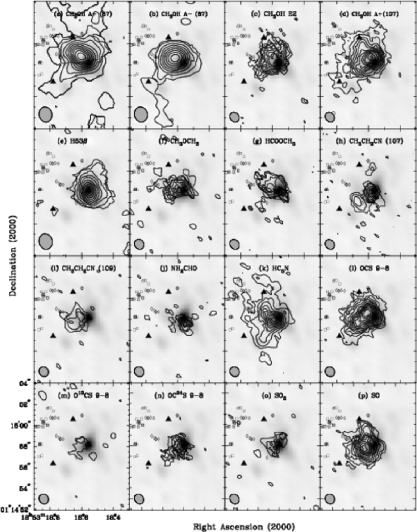
Figure 2: Integrated intensity maps of the spectral lines detected in G34.26+0.15. The species are marked within individual panel. In case of multiple transitions of the same species, the nominal frequency band is also noted. Details of the lines are presented in Table 2. The noise levels (in Jy beam^-1 km s^-1) are : (a) 0.58, (b) 0.40, (c) 0.26, (d) 0.45, (e) 0.61, (f) 0.58, (g) 0.30, (h) 0.48, (i) 30, (j) 0.24, (k) 0.50, (l) 0.35, (m) 0.58, (n) 0.22, (o) 0.46 and (p) 0.32. The contour levels in panels (a), (f), (g), (h), (i), (j), (m), (n) and (o) are in steps of the noise level, starting from twice the noise level. The contour levels in the remaining panels are in steps of twice the noise level, starting from twice the noise level. The negative contours are not shown to simplify the image. The synthesized beams are shown on the left hand corner of each panel. The filled $\Delta$ mark the positions the components A, B, and C (Heaton et al., 1989) of the UC H ii region G34.3+0.2. The squares and diamonds signify positions of H₂O and OH masers respectively (Forster & Caswell, 1989).

Figure 2 shows the integrated intensity maps of the different spectral line emission detected in the region around G34.26+0.15 overlaid with the continuum emission at $\lambda=2.8$ mm and the positions of the H₂O and OH masers detected in the region (Forster & Caswell, 1989). The emission from none of the molecular species coincides with the positions of the H₂O and OH masers.

At a resolution of 1″ the integrated intensity distribution for the different chemical species primarily show three kinds of morphological structures: single-peaked, double-peaked and irregular. Figure 3 shows the positions of the absolute maxima of the integrated intensities for the different species overlaid with the $\lambda=2.8$ mm continuum map of G34.26+0.15. The absolute positional accuracy is estimated to be 0$\farcs$1. We note that it is possible to identify primarily two regions where the maxima due to the transitions of the different species are localized: the first lying slightly to the south-east of the continuum peak and the second lies to the north-east of the 2.8 mm continuum peak.

(a) Single-Peaked : The spectral lines of CH₃OH (with the exception of the $15_{-2}$–15₁ E2 transition), HC₃N, NH₂CHO, SO and OCS, as well as the H53$\beta$ recombination line show well-defined single peaked structures. HCOOCH₃ also shows a single-peaked structure though it is somewhat poorly defined as compared to the rest. Of these spectral lines only the peaks of the H53$\beta$ and the HCOOCH₃ emission coincide with the peak of the continuum at $\lambda=2.8$ mm, while the peaks due to CH₃OH and OCS occur to the north-east of the continuum peak. The peak due to SO lies 1″ to the south-east of the 2.8 mm continuum peak. The peaks of HC₃N and NH₂CHO lie close enough ($\sim$ 0$\farcs$4 south-east) to but not exactly at the position of the 2.8 mm continuum peak. At a first glance, it appears that the more abundant species with higher optical depths tend to show a single-peaked structure. We revisit the question of optical thickness of the lines in Sec. 6.

(b) Double-Peaked : The spectral lines of CH₃CH₂CN and CH₃OCH₃ show rather well-defined double-peaked structure. Figure 3 suggests that the peaks corresponding to the two transitions of CH₃CH₂CN occur at rather different positions. In fact, they correspond to the two peaks that appear in both transitions, with essentially reversed ratios of relative intensities. The double-peaks of CH₃OCH₃ are also not aligned with those of CH₃CH₂CN, as CH₃OCH₃ emission as a whole is somewhat shifted to the north of the continuum peak and extends more along the east-west direction in contrast to the CH₃CH₂CN emission.

(c) Irregular Shaped: The integrated intensity distribution of O¹³CS, OC³⁴S and SO₂ appear to be irregularly shaped and do not have enough signal-to-noise in order to show well-defined peaks. The positions shown in Figure 3 correspond to the absolute maxima within the emitting region and represent the approximate location of the enhancement in emission. These should not be taken too literally as peaks having significance comparable to the peaks for the single-peaked species.

Figure 3 shows that almost all peak positions to the north-east of the continuum peak correspond to single-peaked emission structure. Among the tracers peaking to the south-east, only HC₃N  and SO are single-peaked and CH₃CH₂CN is double-peaked. The remaining tracers have irregular intensity distribution with absolute maxima at the indicated positions.

These two primary locations of the peaks of the spectral lines, (Fig. 3) may either correspond to different emitting clumps or they could be manifestation of the differences in the temperature and density that leads to the variation of the chemical abundances within the same clump. We revisit both these concepts in Sec. 9. In Sec. 7 we derive the chemical abundances of the different chemical species at the two nominal peak positions identified by the CH₃OH $7_{2}$–$6_{3}$A⁺ peak to the north-east and the HC₃N 12–11 peak to the south-east of the continuum peak.

3.4 Velocity Gradients

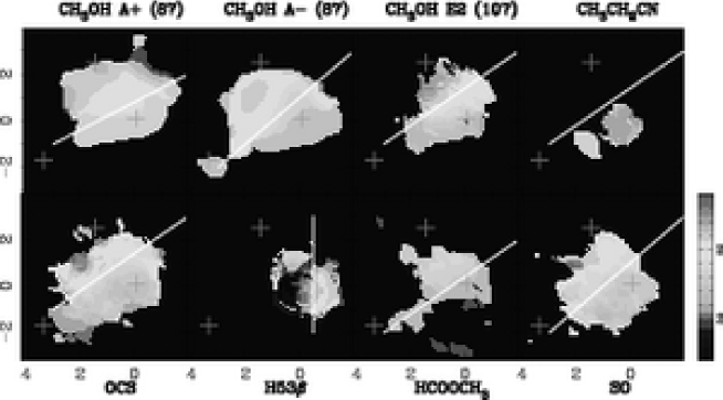
Figure 4: Centroid velocity maps of selected species observed in G34.26+0.15. The colorscale extending between 52 and 64 km s^-1 is shown to the right of the figure. The drawn straight lines show the direction perpendicular to the velocity gradients approximately. The ‘+’ mark the positions the components A, B, and C (Heaton et al., 1989) of the UC H ii region G34.3+0.2.

Figure 4 shows the centroid velocity distribution of some of the selected species for which the signal to noise was sufficient over large areas to generate the maps. With the exception of the hydrogen recombination line and the limited sensitivity CH₃CH₂CN line , the center velocity of all molecular lines changes from 56 km s^-1 in the south-west to 62 km s^-1 in the north-east over a spatial scale of 0.08 pc in a direction approximately with a position angle of 40$\pm 10$°. The direction and magnitude of the velocity gradient match well with other measurements of molecular gas velocity gradients towards G34.26+0.15. Using observations at angular resolutions similar to the present dataset Heaton et al. (1989) derived a velocity gradient of $\geq 50$ km s^-1 pc^-1, while Carral & Welch (1992) and Heaton et al. (1993) observed a velocity gradient of 6$\pm 1$ km s^-1 on 0.3 to 0.75 pc scales. Akeson & Carlstrom (1996) derived a velocity gradient of 15$\pm 5$ km s^-1 on 0.2 to 0.3 pc scales. Watt & Mundy (1999) observed similar velocity gradients as we find, using only CH₃CN. SiO emission primarily tracing outflow activity was not detected at the position of the hot core, it rather appears to surround the hot core (Hatchell et al., 2001). This implies that shocks do not play an important role in regulating the hot core chemistry in G34.26+0.15.

The ionized and molecular gas in G34.26+0.15 show rather different velocity gradients, both in direction and magnitude. The hot molecular gas consistently shows this SW-NE velocity gradient, while the ionized gas has a total gradient of $\approx 35$ km s^-1 in a direction perpendicular to the symmetry axis of the cometary UC H ii region (Gaume et al., 1994). A smaller velocity gradient is detected in the ionized gas parallel to the symmetry axis, i.e. along the east-west direction. In addition, the ionized gas shows typical velocity widths of $\sim 50$ km s^-1 (Garay et al., 1986; Gaume et al., 1994; Sewilo et al., 2004). The hydrogen recombination line, H53$\beta$ shows an emission peak exactly coincident with the continuum peak at $\lambda=2.8$ mm and a velocity gradient similar to the minor component of the velocity gradient as identified in the ionized gas. Similar to all the other recombination lines detected in the region, the H53$\beta$ line has a linewidth much larger than all the other molecular species. These large widths of the recombination lines show conclusively that the ionized gas is driven primarily by the H ii region dynamics.

Comparison of Figs. 2 and 4 show that the observed velocity gradient in the hot molecular gas is along the minor axis of the source emission for all species. This is also consistent with the results of Watt & Mundy (1999). For a core with significant rotation, the velocity gradient is expected to be along the major axis of the source. This argues strongly against the velocity gradients arising due to the gravitationally bound rotation of a circumstellar slab or disk as was proposed by Garay et al. (1986). Several authors have interpreted the observed velocity distribution of the UC H ii region G34.26+0.2C in terms of mainly two models: the moving star bow shock model and the champagne outflow model. However, Gaume et al. (1994) point out that none of these models satisfactorily explain the observed velocities in the region. These authors proposed a model in which the velocities in the region are governed by the stellar winds from the components A and B. Further, the ionized gas which is photoevaporated directly from the hot, dense UC molecular core by the exciting star of the cometary H ii region G34.26+0.2C, flows from the molecular core toward a region of lower density to the west. In this model, it is further proposed that the molecular core and the components A and B are at a slightly larger distance from the Earth than G34.3+0.2C. The velocity pattern derived from the various species observed here is consistent with the “wind and photoevaporation” model proposed by Gaume et al. (1994), and this further strengthens the conclusions of Watt & Mundy (1999), which were derived based only on the velocity patterns of CH₃CN.

4 Energetics of the hot core in G34.26+0.15

Hot cores are typically proposed to be precursors of high mass stars (e.g. Cesaroni, 2005). The center of the hot core is identified with a collapsing, and rapidly accreting high mass protostar. High angular resolution mid-infrared (MIR) observations have successfully detected the energizing sources for several hot cores like G11.94-0.62, G45.07+0.13, G29.96-0.2 etc. (De Buizer et al., 2002, 2003). Using sub-arcsecond resolution centimeter and millimetre molecular line and continuum observations the existence of multiple deeply embedded UC and hypercompact H ii regions contributing to the formation of the HMCs G10.47+0.03 and G31.41+0.31 have been substantiated (Beltrán et al., 2004, 2005). Most of the HMCs thus represent a stage in the evolutionary sequence of massive protostars.

However, in the case of the hot molecular gas in G34.26+0.15 the existing continuum observations in mid-infrared, far-infrared, sub-millimeter and millimeter have consistently shown the peak of the dust emission to be coincident with the UC H ii region component C and not at the position of the hot core (Hunter et al., 1998; Campbell et al., 2000, 2004). In particular, using MIR observations with 1–2″ resolution (De Buizer et al., 2003) have reported non-detection of any MIR source associated with the HMC in G34.26+0.15. Thus G34.26+0.15 similar to the Orion Compact Ridge and W3(OH) (Wyrowski et al., 1999) represents the alternative scenario for hot cores, which are externally heated and viewed upon as manifestation of gas shocked and heated by the expanding ionization front and the stellar winds arising from the H ii regions. Medium angular resolution MIR and FIR observations further suggest that the HMC is isolated from the component C of the H ii region and is heated by stellar photons from A and B components and not shocks (Campbell et al., 2000, 2004). Watt & Mundy (1999) compared the CH₃CN  and C¹⁸O peaks with the NH₃ peaks seen in arcsecond resolution observations by Heaton et al. (1989) and found that none of the peaks coincide with either component C of the H ii region or with each other. These suggest that the hot molecular gas detected in G34.26+0.15 traces a layer of a core that is being externally heated by shocks and stellar photons. However, non detection of SiO emission from the position of the hot core rules out any significant role played by shocks in determining the hot core chemistry (Hatchell et al., 2001).

The arcsecond resolution continuum and molecular line observations presented in this paper provide further evidence to this proposed model of the hot core in G34.26+0.15 being externally heated. The continuum map at 2.8 mm shows a single peak coincident with the radio continuum peak, and it is offset from the peaks of all molecular lines. The molecular line maps extending over a region of 9″$\times$12″ ($\alpha\times\delta$) show that (i) the emission from different species are not centrally peaked, (ii) the molecular peaks are not co-spatial, (iii) none of the molecular line emission peaks at the continuum peak and (iv) none of the molecular line peaks coincide with the H₂O and OH masers, tracing locations of shocks due to the propagation of the ionization front from the UC H ii regions, detected in the region (Forster & Caswell, 1989).

The relative offsets between the peaks in the different molecular line emission further brings out the possibility of there being multiple HMCs within the beam. We note that the NE and the SE peaks detected in the G34.26+0.15 region are separated along the north-south direction by 0$\farcs$8, which at a distance of 3.7 kpc translates to 0.014 pc. For comparison, the Hot Core and the Compact Ridge regions in the Orion-KL cloud at a distance of 450 pc are separated by 0.018 pc. We consider the angular resolution of the present observations to be insufficient to either clearly resolve or rule out the possibility of the two peaks being two different cores. These results differ substantially from the single-dish observations which have so far suggested that the emission from the different molecular species originate from within a single bound core.

The observations of G34.26+0.15 presented here, with the highest angular resolution to date, suggest multiple externally heated HMCs, a hypothesis which is a matter of further study. In the absence of observations of multiple transitions of molecular species at 1″ resolution, it is not possible to derive the density and temperature distributions appropriate to decipher factors contributing to the relative offsets of the different emission peaks. Availability of such temperature and density profiles is also crucial for deriving accurate estimates for the abundance profiles for the detected complex molecular species.

5 Available chemical models for hot cores and G34.26+0.15

Existing and recent high angular resolution observations of the HMC associated with G34.26+0.15 strongly favour that the source is externally heated. However there are no observations available that constrain (i) the geometry of the hot core material with respect to the external heating source; (ii) the density structure of the core material, e.g. whether it shows a simple gradient in a particular direction or it is clumpy or it is a uniform density swept up region; or (iii) the geometry and multiplicity of the core along the line of sight. We propose the present dataset as a building block for future observations which would help clarify some of the outstanding issues.

The rather “unconventional” and complicated geometry of the HMC associated with G34.26+0.15 poses further challenge to deriving a consistent chemical model for the source. All existing chemical models for HMCs, including those constructed specifically for G34.26+0.15 (e.g. Millar et al., 1997; Nomura & Millar, 2004) explicitly consider a centrally energized spherical cloud forming a massive protostar in two stages involving collapse to high densities ($\sim 10^{7}$ cm^-3) followed by a warm-up phase resulting in the rich chemistry of the hot cores. The models for the HMC in G34.26+0.15 are primarily based on single dish observations and assume that the source consists of a hot ultracompact core (UCC) with a radius less than 0.025 pc and $n(H_{2})=2\times 10^{7}$ cm^-3, a compact core (CC) with a radius of about 0.1 pc and a density of 10⁶ cm^-3, surrounded by a massive halo extending out to 3.5 pc with a H₂ density that falls off as r^-2 (e.g. Millar et al., 1997, and the references therein). The latest chemical model for G34.26+0.15 by Nomura & Millar (2004) is more sophisticated in terms of using the density and temperature profiles derived from the dust continuum observations. These density and temperature profiles are subsequently used as inputs for the chemical model. However, the density and temperature distributions are primarily constrained by single-dish continuum observations and the model considers a centrally peaked spherically symmetric structure that is isothermal up to a radius of 0.05 pc ($\sim 3$″). Further it assumes the core of the region to be collapsing to form a massive protostar. Most of these assumptions do not conform to the results of high angular resolution molecular line observations presented in this paper and also by Watt & Mundy (1999) and Heaton et al. (1989). Similar arguments may be invoked to show the inappropriateness of the radiative transfer models developed by Hatchell & van der Tak (2003) for the HMC in G34.26+0.15.

6 Estimate of Kinetic Temperature

In the absence of high resolution multi-line spectroscopic observations suitable to derive the temperature and density distributions, we have adopted a simplistic approach to derive an estimate of the kinetic temperature from the observed brightness temperatures.

Using the brightness temperatures of OC³⁴S 9–8 (50 K) and OCS 9–8 (96 K) at the position of the intensity peak of OC³⁴CS (Table 3), and the relative abundance of the isotopomers ${}^{32}S$/${}^{34}S$ $\sim 22$ (Wilson & Rood, 1994) we derive $\tau_{34}=0.7$ and $\tau_{32}=15.4$. Hence OCS 9–8 is optically thick and its peak brightness temperature (167 K) is a reasonably good estimate of the gas kinetic temperature. We further note that the peak brightness temperature of CH₃OH 3₁–4₀ A⁺, the brightest and the most optically thick of the methanol lines observed here is 187 K: the peak brightness temperatures of SO and HC₃N are 147 K and 143 K, respectively. Thus beyond the calculated high opacity values of OCS 9–8, the rather high peak brightness temperatures of CH₃OH 3₁–4₀ A⁺, SO and HC₃N suggest that all these lines are optically thick and their peak brightness temperatures provide a firm lower limit to the true kinetic temperature of the UCC of G34.26+0.15. Based on these, we estimate the kinetic temperature to be 160$\pm 30$ K and use 160 K for the subsequent analysis.

Most of the available estimates of kinetic temperature of the hot core region G34.26+0.15 are rotation temperatures derived using a variety of molecules. Based on an LVG analysis of CH₃CN (Watt & Mundy, 1999) derived a gas temperature between 80–175 K, while using the K-ladder of the same molecule Akeson & Carlstrom (1996) estimated a kinetic temperature of $250\pm 100$ K. Millar et al. (1995) derived a rotation temperature of 125 K from C₂H₅OH observations, while Henkel et al. (1987) derived a rotation temperature of $225\pm 75$ K from ammonia observations.

The errorbars in the kinetic temperatures available from literature are rather large and they are all consistent with our derived value of 160$\pm 30$ K. The higher angular resolution of our observations better probe the small clumps in contrast to the other observations. We note that the molecules of which rotational transitions were used to derive the kinetic temperatures have similar dipole moments. However, comparison with temperatures derived from single dish observations with the present results is uncertain due to multiple issues: beam dilution, contamination from large scale emission, etc.

7 Column Densities of different species

We have derived the column densities of the different observed species assuming Local Thermal Equilibrium (LTE), the kinetic temperature to be 160 K, and the observed transitions (with the exception of OCS 9–8) to be optically thin. The assumption of a single temperature instead of a temperature profile leads to inaccuracies in our estimates of abundances. However, given the non-centrally peaked geometry of the hot molecular gas as detected in our observations and the lack of dust continuum data, as well as observations of multiple spectral lines constraining the density and temperature profiles, resolving these uncertainties is beyond the scope of this paper. We propose the use of these abundances in combination with upcoming high angular resolution complementary observations in order to provide constraints for future chemical models.

Based on the peak brightness temperatures presented in Table 3 we conclude that in all likelihood HC₃N, SO, and CH₃OH A⁺ $3_{1}$–$4_{0}$ transitions are also optically thick. In the absence of observations of rarer species, we use the estimated column densities as lower limits and/or guidelines. For both CH₃OH and CH₃CH₂CN we adopt the largest among the column densities derived from the different observed transitions. The CH₃OH $7_{2}$–$6_{3}$ A^- transition gives the highest column density and it has a peak brightness temperature of 82 K, which suggests that it is still optically thin. The column density of OCS 9–8 is derived by using the OC³⁴S column densities and assuming the relative Galactic abundance of ${}^{32}S$/${}^{34}S$ $\sim 22$. Table 4 presents the observed column densities and abundances of the different species at the positions of the north-eastern (NE) and south-eastern (SE) peaks, abundances of NH₃ (Heaton et al., 1989), CH₃CN (Watt & Mundy, 1999), along with abundances of different species in other “prototypical” hot cores.

The present dataset does not provide an independent estimate of the total molecular hydrogen column density, $N_{\rm H_{2}}$, in the ultracompact core (UCC; Heaton et al., 1993) of G34.26+0.15. Estimates of $N_{\rm H_{2}}$ in the core, mostly based on a number of single-dish and interferometric observations of different chemical species, vary by almost an order of magnitude. Using the peak NH₃ abundance of 2$\times$10^-5 (Millar et al., 1997) and the observed NH₃ column density of 7$\times$10¹⁸ cm^-2 (Heaton et al., 1989), Watt & Mundy (1999) estimated $N_{\rm H_{2}}$ to be 4$\times 10^{23}$ cm^-2. In contrast based on NH₃ (Heaton et al., 1989) and CH₃CN (Akeson & Carlstrom, 1996) observations, the $N_{\rm H_{2}}$ is estimated to be 3–$7\times 10^{24}$ cm^-2. The lower H₂ column densities deduced by Watt & Mundy (1999) are however consistent with the non-detection of C¹⁸O at the center of the core. Following Watt & Mundy (1999) here we adopt the $N_{\rm H_{2}}$ of the UCC within G34.26+0.15 to be 4$\times$10²³ cm^-2 in order to calculate the observed abundances of the observed chemical species relative to molecular hydrogen (Table 4). The CH₃CN and NH₃ observations that have angular resolution comparable to our observations justify the adopted value of $N_{\rm H_{2}}$.

The derived column densities of the complex molecules like CH₃OH, HCOOCH₃, CH₃CH₂CN and CH₃OCH₃ agree reasonably well with the previous observations (at 13″$\times$8″ resolution) by Mehringer & Snyder (1996). Following Table 4 we find that at the two rather clearly segregated peak positions within the inner regions of the HMC in G34.26+0.15, the abundances of CH₃OCH₃, CH₃CH₂CN, HC₃N, NH₂CHO, and SO₂ differ by factors $<3$.

8 Hot core chemistry in G34.26+0.15

We have detected several of the N-, O- and S-bearing parent and daughter molecules in the G34.26+0.15 hot core region. Here we discuss the relative abundances of the different species in the light of the abundances observed in a few well-known hot core regions (Table 4). We also compare the abundances relative to a few well-known chemical models for hot cores, these include: chemical models for G34.26+0.15 by Millar et al. (1997) and Nomura & Millar (2004), both at $t_{\rm core}$ = 10⁴ yr after the grain mantle evaporation; and the model for the Orion compact ridge at $t_{\rm core}$ = 3.3$\times 10^{4}$ yr by Caselli et al. (1993). The model by Caselli et al. (1993) though not fine-tuned for G34.26+0.15, is relevant because previous chemical study by Mehringer & Snyder (1996) suggested that the observed abundances can be explained reasonably well by this model at $t_{\rm core}=10^{4}$ yr.

The chemical model for G34.26+0.15 presented by Nomura & Millar (2004) is essentially an improvement of the model by Millar et al. (1997) in terms of using latest collision rates and chemistry. However for the model by Nomura & Millar (2004) column densities are available only for the entire source, rather than explicitly for the UCC or the inner regions of the HMC in G34.26+0.15. Since, the enhanced angular resolutions of the present BIMA observations enables us to probe the inner regions of the HMC directly, the column density calculations for the UCC by Millar et al. (1997) are still relevant for our work. Further we note the column densities of the entire source (core+halo) as estimated by these two models agree reasonably well.

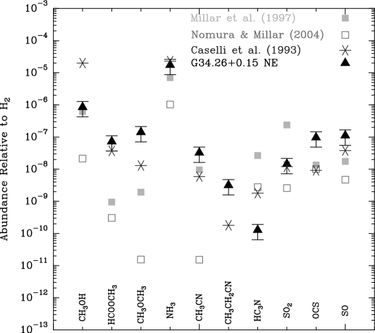
Figure 5: Comparison of column densities observed at the north-eastern (NE) peak of G34.26+0.15 with different chemical models. The observed relative abundances are derived by assuming $N_{\rm H_{2}}$ = 4$\times 10^{23}$ cm^-2. The errorbars correspond to 50% errors in abundance estimates. Caselli et al. (1993) corresponds to the chemical model for the Orion Compact Ridge at $t_{\rm core}=3.3\times 10^{4}$ yr. Millar et al. (1997) corresponds to the chemical model for the ultracompact core, for which $N_{\rm H_{2}}$ = 2.7$\times 10^{23}$ cm^-2 at $t_{\rm core}=10^{4}$ yr. Nomura & Millar (2004) corresponds to a chemical model for the entire source G34.26+0.15, for a line of sight through the center of the core at $t_{\rm core}=10^{4}$ yr, with $N_{\rm H_{2}}$ = 3.6 10²⁴.

Figure 5 compares the abundances of the different species relative to the molecular hydrogen abundance as observed at the NE peak of G34.26+0.15 with abundances predicted by the different chemical models. In the following sections we discuss the abundances of the O-, N- and S-bearing molecular species separately and compare them with abundances seen in other hot cores.

8.1 Oxygenated species

We have detected CH₃OH, CH₃OCH₃ and HCOOCH₃. Figure 5 shows that there is a huge discrepancy between the abundances of CH₃OH as predicted by Caselli et al. (1993) and Millar et al. (1997), with the latter model reproducing the observed abundances in G34.26+0.15 exactly. All the chemical models predict the relative abundance HCOOCH₃/CH₃OH to be between 10^-3 and 10^-2 and do not reproduce the high abundance ratio of 0.1 as observed in most hot cores (Table 4). On the other hand a relative abundance of CH₃OCH₃/CH₃OH $\sim 10^{-3}$ is predicted by all the models, which is more or less consistent with the observed range of values in the other hot cores. Most of the chemical models for hot cores, including those considered in this paper rely solely on gas-phase chemistry to account for the formation of the large O-bearing complex molecules. However, Horn et al. (2004) have shown that the gas-phase processes are highly inefficient in producing HCOOCH₃ and can never reproduce the observed abundances. Recently Garrod & Herbst (2006) has proposed a slower warm-up phase of the hot core and a combination of grain-surface and gas-phase chemistry in the hot cores, which better reproduce the observed abundances of HCOOCH₃.

8.2 Nitrogenated Species

Table 4 suggests that the abundances of the N-bearing species, NH₃, CH₃CN, CH₃CH₂CN, HC₃N, and NH₂CHO in G34.26+0.15 lie within the range of values seen in other hot cores.

Discovery of NH₃ ice has lead to the conclusion that NH₃ is indeed a parent species evaporated from the grain mantle. Presence or absence of NH₃ in the grain mantle plays an important role in determining the abundances of the different daughter species (Rodgers & Charnley, 2001). Figure 5 suggests that while Caselli et al. (1993) reproduces the NH₃ abundance seen in G34.26+0.15; both Millar et al. (1997) and Nomura & Millar (2004) fall short by a factor of $\sim 10$ or more, with the latter model being much worse.

CH₃CN, a symmetric top molecule, is likely to form via radiative association of CH${}_{3}^{+}$ with HCN or CN with CH₃ (Charnley et al., 1992; Millar et al., 1997). The chemical models for the UCC of G34.26+0.15 (Millar et al., 1997) and the Orion Compact Ridge (Caselli et al., 1993) predict CH₃CN abundances 30–50 times lower than the observed value in G34.26, while the core+halo model of Nomura & Millar (2004) predicts an even lower CH₃CN abundance (Fig. 5).

The high abundances of nitrile molecules like CH₃CH₂CN as found in many hot cores cannot be reproduced by gas phase reactions alone. Hydrogenation of accreted HC₃N and CH₃CN to produce CH₃CH₂CN that when evaporates, is proposed to be a more viable path for CH₃CH₂CN formation in hot cores (Charnley et al., 1992; Caselli et al., 1993). The chemical model for Orion Compact Ridge by Caselli et al. (1993) predicts an abundance that is 10 times lower than observed in G34.26. No predictions for the abundance of CH₃CH₂CN are available from the other two chemical models in consideration here.

HC₃N is thought of as a cold-cloud tracer but should also be formed efficiently in the hot gas if C₂H₂ is evaporated from grain mantles (Millar et al., 1997). Figure 5 shows that all the chemical models predict an HC₃N abundance larger by more than a factor of 100 than the value observed in G34.26. This is consistent with our estimate that HC₃N is optically thick (Sec. 6) in G34.26+0.15.

NH₂CHO is most likely formed by atom addition to HCO on grain mantles and then evaporate (Tielens & Charnley, 1997). Bernstein et al. (1995) found NH₂CHO to be formed upon UV photolysis and warm-up of H₂O:CH₃OH:CO:NH₃= 100:50:10:110 mixture. However, most of the chemical models so far do not consider either CH₃CH₂CN or NH₂CHO as parent species and there are no predictions of abundances available so far.

8.3 Sulphuretted species

Based on single-dish observations of G34.26+0.15 and subsequent chemical modeling, Hatchell et al. (1998) inferred that the OCS emission, which requires rather high excitation energy, can not be produced in the extended halo; the rotation temperature derived from SO₂ warrants a core origin; and the SO lines are more likely to arise from the halo. We estimate both OCS and SO to be optically thick and to have peak brightness temperatures characteristic of the inner regions. Table 4 shows that abundance of OCS as observed in G34.26+0.15 is larger than those observed in many hot cores. The abundance of SO in G34.26+0.15 is similar to that in Orion, while Sgr B2(N) and G327.6–0.3 show much lower abundances. Note that the SO abundance derived here is likely a lower limit due to the optically thick SO line. The SO₂ abundance in G34.26+0.15, is similar to the abundance seen in Sgr B2(N) and both are lower by a factor of 10 than the values seen in Orion and G327.3–0.6. It was initially pointed out by Charnley (1997) and Hatchell et al. (1998) that the relative abundance ratios of SO, SO₂ and H₂S could be used to estimate the age of the hot cores of the massive protostars. However, Wakelam et al. (2004) has re-considered this issue and conclude that none of these ratios can be used by itself to estimate the age, since the ratios depend at least as strongly on the physical conditions and on the adopted grain mantle composition as on time.

Figure 5 shows that all the chemical models under consideration here predict very similar OCS abundances, although somewhat less than that observed in G34.26+0.15. The model by Caselli et al. (1993) reproduces the observed SO abundance in G34.26+0.15 reasonably well, while the other two models predict abundances lower by factors of 5–10. Since we estimate SO in G34.26+0.15 to be optically thick, it is hard to reconcile to the higher abundance derived observationally. The model by Caselli et al. (1993) reproduces the observed abundances of SO₂ for G34.26+0.15, while the models by Millar et al. (1997) and Nomura & Millar (2004) respectively overestimates and underestimates the observed values.

8.4 Summary of comparison with chemical models

None of the chemical models considered here reproduce the abundances of all the observed species satisfactorily. These models like all the other chemical and radiative transfer models for HMCs assume the energizing source to be at the center, with centrally peaked temperature and density profiles. In addition, there are reasonable arguments in favor, as well as, against the complex molecule formation mechanisms (grain-mantle evaporation, grain-surface chemistry, gas-phase chemistry). Thus, from the physical point of view all these models are not directly applicable to G34.26+0.15, which as our observations show is externally heated and additionally might be harboring multiple unresolved HMCs.

There are two main uncertainties in our estimates of the column densities of the different species: (i) we have assumed a single kinetic temperature, rather than a temperature profile, the value of which may also be off by 50 K for some of the species and (ii) the $N_{\rm H_{2}}$ estimate is also not accurate. Both of these uncertainties can only be addressed with complementary observations at comparable angular resolutions. The errorbars drawn at the 50% level in Fig. 5 attempt to quantify these uncertainties in addition to the statistical errors and the errors in absolute calibration. Since the difference in abundances between the NE and SE peaks of G34.26+0.15 never exceeds a factor of 3 and the discrepancy between the observed and predicted abundances are of the order of factors of 10 or more, our conclusions would not have been significantly different had we compared the observed abundances at the SE peak with the model predictions. Further, we have shown that the abundances observed in G34.26+0.15 are not atypical compared to other Galactic hot cores. Thus, discrepancies by factors of 10 to 100 between the abundances observed in G34.26+0.15 and the predictions of the chemical models can not be explained by the estimated errors in abundance calculations. Given the inappropriateness of the existing chemical models and uncertainties in the derived relative abundances we consider any age/timescale related discussion for the HMC in G34.26+0.15 beyond the scope of this paper.

9 Discussion

Despite the present consensus on the contemporaneous existence of NH₃ and CH₃OH bearing grain mantles, chemical differentiation in hot core regions is also well-established from observations. Such chemical differentiation was prominently noticed in the two clumps in the Orion-KL cloud core, very close to the luminous and massive young stellar object, IRc2: the Hot core and the Compact Ridge. While the warmer and denser Hot Core shows unusually high abundances of H-rich complex N-bearing molecules like CH₂CHCN and CH₃CH₂CN, the Compact Ridge is characterized by high abundances of large oxygen-bearing molecules like CH₃OH, HCOOCH₃ and CH₃OCH₃. However, later observations of the Orion-KL hot cores by Sutton et al. (1995) suggest that the chemical differentiation is probably not as drastic as it was first thought to be. Similar chemical differentiation is observed between the two hot cores W3(H₂O) and W3(OH) in the W3 region (Wyrowski et al., 1997, 1999). These sources are spatially offset by about 0.06 pc and yet they exhibit clear signs of N/O differentiation. Both sources show emission from CH₃OH, H₂CO, CH₃OCH₃, and HCOOCH₃, but only the maser source shows significant emission from CH₃CH₂CN, HC₃N, and SO2 (Wyrowski et al., 1997, 1999), as well as from HCN (Turner & Welch, 1984) and CH₃CN (Wilson et al., 1993).

Several chemical models have partially explained the chemistry of both the Hot Core & the Compact Ridge (Caselli et al., 1993; Charnley et al., 1992) in Orion. Rodgers & Charnley (2001) have shown that the evaporation of NH₃ rich grain mantles inhibit high abundances of O-bearing large molecules, though the already injected alcohols remain abundant for much longer. This leads to the formation of N-rich hot cores. Rodgers & Charnley (2003) further showed that in collapsing cores both N-rich and O-rich species tend to co-exist. However, it might be possible to derive the age of the cores based on the relative abundance of the two types of species because CH₃OCH₃ is found to be more abundant at earlier times whereas HCN and CH₃CN form later on (Rodgers & Charnley, 2003). Observational detection of large number of daughter species in hot cores suggest that the chemical timescale needs to be shorter than the dynamical timescale, i.e., the cores need to be gravitationally supported up to 10⁴ yrs (Rodgers & Charnley, 2003).

Within the inner regions of G34.26+0.15 we find that the N-bearing species tend to peak to the south-east, while the peaks of the O-bearing species are concentrated to the north-east of the continuum peak. The NE and the SE peaks are primarily separated along the north-south direction by 0$\farcs$8, which at a distance of 3.7 kpc translates to 0.014 pc. For comparison, the Hot Core and the Compact Ridge regions in the Orion-KL cloud at a distance of 450 pc are separated by 0.018 pc. Thus, given the larger distance to the source and the angular resolution of the present observations, the possibility of the two emission peaks actually belonging to two different cores, one being N-rich and the other being O-rich, can not be ruled out. Although the two peak positions in G34.26 do not show large difference in CH₃OH abundances, differences in the abundances of CH₃OCH₃, CH₃CH₂CN, HC₃N and NH₂CHO show contrasts quite similar to what is seen in Orion-KL (Sutton et al., 1995). Additional high angular resolution observations of molecular lines are required to derive a better estimate of the temperature distribution, in order to improve the derived abundances at the two peak positions seen within the inner regions of the HMC in G34.26+0.15.

10 Summary

We have presented high angular resolution mapping observations of the HMC in G34.26+0.15 tracing different chemical species characteristic of hot cores. The higher angular resolution enables us to probe the inner regions of the hot molecular gas. The observations presented here is only a first step and needs to be augmented by observations of standard temperature and density sensitive molecular transitions to constrain the physical attributes of the region which can then be used as constraints for future chemical models.

We do not detect any evidence for an energizing source at the center of the hot core, the continuum peak at 2.8 mm is consistent with the free-free radio continuum emission from component C of the UC H ii region. The intensity distribution of the various molecular tracers do not peak at the same position, the peaks of none of the distributions is located either at the position of the continuum peak or the positions of the H₂O and OH masers. The temperature and density distributions of the inner regions of the hot cores can not be determined from the present observations. Based on intensity and velocity distribution, only component C, the most evolved of the H ii regions associated with G34.26+0.15 appears to influence the energetics of the hot molecular gas. The kinematics of the hot core as derived from the velocity distribution of the molecular tracers is not strongly influenced by the H ii region dynamics.

Within the inner regions of the hot core in G34.26+0.15 we find that the nitrogen and oxygen-bearing species tend to show a dichotomy and peak at different positions, separated by 0$\farcs$8, the spatial separation being similar to the two hot/warm cores identified in the Orion. We propose that as in Orion and in W3(OH), (i) these peak positions may indeed be separate regions of chemical enrichment, resolution of which would require even higher angular resolution observation and (ii) may arise due to the external influence of the neighboring H ii regions. We have estimated the abundances of the observed molecular species at the two peak positions assuming a single kinetic temperature of 160 K under conditions of LTE.

The high angular resolution observations presented here, provides overwhelming evidence in favour of the hot molecular gas at spatial scales of 0.018 pc being externally heated. This together with the clumpiness of the region and possible existence of multiple HMCs in the region, implies geometries more complicated than those considered by the state-of-art chemical models. For the sake of completeness, we follow Wyrowski et al. (1999) to derive a crude upper limit for the luminosity of the internal energizing source if any, using the kinetic temperature derived in this paper and Stefan-Boltzmann law. The luminosity of the hypothetical and so far undetected internal source is estimated to be 8.9$\times$10⁴ $\mathrm{L}_{\odot}$ and this corresponds to a O7.5 ZAMS star (Panagia, 1973).

Comparison of the abundances observed in G34.26+0.15 with currently available somewhat inappropriate chemical models for hot cores by Caselli et al. (1993), Millar et al. (1997), and Nomura & Millar (2004) suggest that the nitrogen richness of the region can only be explained by the evaporation of ammonia-rich ice-mantles. However, this implies that the abundances of the oxygenated daughter species be suppressed in the presence of ammonia, which is not the case in G34.26+0.15. This can mean any of the following (i) the oxygenated species in question are also formed on grain mantles, (ii) the two regions are actually separate from each other or (iii) there may be additional gas-phase processes which can progress efficiently even in the presence of ammonia to create high abundances of oxygenated daughter species, which the chemical models do not yet consider. Comparison of abundances observed in a few hot cores (in addition to G34.26+0.15) and the chemical models show that the chemical models do not yet consistently explain the abundances of all species in any of the hot cores. The complicated geometry of G34.26+0.15 makes direct comparison of the observed abundances with the chemical models even more difficult.

One of the major caveats of the estimates of the abundances presented here in the hot molecular gas is the assumption of a single kinetic temperature characterizing the emission of the different species. This is a consequence of the lack of complementary observations of molecular species at high angular resolutions to study the temperature and physical structure of the hot molecular gas. In order to understand the true nature of the different peak positions in G34.26+0.15 as identified in the BIMA data and to provide proper physical constraints for the chemical models for the region, sub-arcsecond resolution observations are necessary.

Table 1: Details of BIMA observations of G34.26+0.15

Frequency	Configuration	Date	Tsys
GHz			K
87	A	23 Dec 1999	180
	B	26 Feb 2000	450
107	A	29 Jan 2000	200
	B	10 Mar 2000	350
109	A	6 Feb 2000	250
	B	13 Mar 2000	300

Table 2: Spectroscopic parameters of molecular transitions detected by 1″ resolution BIMA observations of G34.26+0.15

Species	Transition	Frequency	E${}_{u}/k$T	$S_{ij}$
		GHz	K
$\rm CH_{3}OH$	$7_{2}$–$6_{3}$ A-	86.6155080	102.7	0.644
	$7_{2}$–$6_{3}$ A+	86.9030180	102.7	0.644
	$3_{1}$–$4_{0}$ A+	107.0138500	28.36	1.43
	$15_{-2}$–$15_{1}$ E2	107.15992	305	1.24
$\rm HCOOCH_{3}$	$8_{2,6}$–$7_{2,5}$ E	103.46659	24.66	19.992
$\rm CH_{3}OCH_{3}$	$13_{1,12}$–$13_{0,13}$  EA+AE	105.7683438	86.02	5.405
$\rm NH_{2}CHO$	$5_{2,4}$–$4_{2,3}$	105.972601	27.2	4.2
$\rm OC^{34}S$	9–8	106.7873889	25.7	9.0
$\rm O^{13}CS$	9-8	109.1108477	26.2	9.0
OCS	9–8	109.4630630	26.28	9.0
$\rm CH_{3}CH_{2}CN$	$12_{2,11}$–$11_{2,10}$	107.0435270	37.91	11.662
	$12_{1,11}$–$11_{1,10}$	109.6502630	35.42	11.906
$\rm SO_{2}$	$27_{3,25}$–$26_{4,22}$	107.0602085	369.5	3.102
$\rm HC_{3}N$	12–11	109.1736340	34.07	12.0
SO	$3_{2}$–$2_{1}$	109.2522200	21.05	1.510

Table 3: Basic observational results of the chemical survey towards G34.26+0.15. Synthesized beam sizes at 87 GHz, 107 GHz and 109 GHz are 1$\farcs$48$\times$1$\farcs$25, 1$\farcs$02$\times$0$\farcs$85 and 0$\farcs$99$\times$0$\farcs$89 respectively.

Line	Beam	$F_{\rm peak}$	$T_{\rm B,peak}$	$v_{\rm cen}$	$v_{\rm fwhm}$	RMS
	(arcsec)	(Jy beam-1)	(K)	(km s-1)	(km s-1)	(mJy beam-1)
H53$\beta$	1$\farcs$48$\times$1$\farcs$25	0.454	42	$56.0\pm 1.8$	$45.2\pm 4.7$	66.3
$\rm CH_{3}OH$ $7_{2}$–$6_{3}$ A-	1$\farcs$48$\times$1$\farcs$25	0.934	82	$59.1\pm 0.3$	$6.2\pm 1.0$	69.1
$\rm CH_{3}OH$ $7_{2}$–$6_{3}$ A+	1$\farcs$48$\times$1$\farcs$25	0.952	83	$59.3\pm 0.3$	$7.0\pm 0.5$	69.6
$\rm HCOOCH_{3}$ $8_{2,6}$–$7_{2,5}$ E	1$\farcs$02$\times$0$\farcs$85	0.240	31	$56.3\pm 2.0$	$4.7\pm 1.0$	35.6
$\rm CH_{3}OCH_{3}$ $13_{1,12}$–$13_{0,13}$	1$\farcs$02$\times$0$\farcs$85	0.218	26	49.3	…	55.1
$\rm NH_{2}CHO$ $5_{2,4}$–$4_{2,3}$	1$\farcs$02$\times$0$\farcs$85	0.383	46	$55.9\pm 0.3$	$7.3\pm 07$	106.
$\rm OC^{34}S$ 9–8	1$\farcs$02$\times$0$\farcs$85	0.394	50	$56.0\pm 0.3$	$4.0\pm 0.7$	86.1
$\rm CH_{3}OH$ $3_{1}$–$4_{0}$ A+	1$\farcs$02$\times$0$\farcs$85	1.48	187	$58.4\pm 0.2$	$6.0\pm 0.3$	44.9
$\rm CH_{3}CH_{2}CN$ $12_{2,11}$–$11_{2,10}$	1$\farcs$02$\times$0$\farcs$85	0.365	46	$55.9\pm 0.1$	$4.4\pm 0.5$	45.3
$\rm SO_{2}$ $27_{3,25}$–$26_{4,22}$	1$\farcs$02$\times$0$\farcs$85	0.198	25	$56.6\pm 1.0$	$6.3\pm 1.5$	45.3
$\rm CH_{3}OH$ $15_{-2}$–$15_{1}$ E2	1$\farcs$02$\times$0$\farcs$85	0.643	81	$60.0\pm 0.1$	$6.3\pm 0.3$	94.9
$\rm O^{13}CS$ 9-8	0$\farcs$99$\times$0$\farcs$89	0.165	20	55.6	…	67.5
$\rm HC_{3}N$ 12–11	0$\farcs$99$\times$0$\farcs$89	1.23	143	$56.5\pm 0.1$	$6.4\pm 0.1$	64.3
SO $3_{2}$–$2_{1}$	0$\farcs$99$\times$0$\farcs$89	1.27	147	$58.0\pm 0.1$	$4.6\pm 0.3$	123.1
OCS 9–8	0$\farcs$99$\times$0$\farcs$89	1.44	167	$58.4\pm 0.2$	$5.2\pm 0.4$	127.0
$\rm CH_{3}CH_{2}CN$ $12_{1,11}$–$11_{1,10}$	0$\farcs$99$\times$0$\farcs$89	0.360	42	$58.5\pm 0.6$	$5.0\pm 1.3$	65.2

Table 4: Chemical abundances of the species observed towards G34.26+0.15. Assumed $T_{\rm kin}$ = 160 K. $N$ and $X$ refer to column densities and abundances relative to molecular hydrogen respectively. NE and SE refer to the north-eastern and south-eastern peaks respectively. Column densities of optically thick lines of OCS 9–8 has been derived from OC³⁴S assuming ³²S/³⁴S = 22. The relative abundances for the compact core have been calculated using $N_{\rm H_{2}}$= 4$\times 10^{23}$ cm^-2 (Watt & Mundy, 1999). $a(b)$ refers to $a\times 10^{b}$. Considering the errors in absolute calibration, statistical errors, errors due to the assumption of a single $T_{\rm kin}$, and the error in $N_{\rm H_{2}}$ we conservatively estimate an error of 50% in the calculated abundances.

Species	$N_{\rm NE}$	$X_{\rm NE}$	$N_{\rm SE}$	$X_{\rm SE}$	OMC	OMC	SgrB2 (N)	G327.3–0.6
	cm-2		cm-2		Hot Core	Compact Ridge
CH3OH	3.4(17)	8.5(0-7)	2.6(17)	6.4(0-7)	1.4(0-7)	4.0(0-7)	2.0(0-7)	2.0(0-5)
HCOOCH3	2.9(16)	7.3(0-8)	2.7(16)	6.8(0-8)	1.4(0-8)	3.0(0-8)	1.0(0-9)	2.0(0-6)
CH3OCH3	5.7(16)	1.4(0-7)	3.4(16)	8.5(0-8)	8.0(0-9)	1.9(0-8)	3.0(0-9)	3.4(0-7)
NH3	7.0(18)	1.8(-5)	…	…	6.7(0-8)	5.7(0-7)	…	…
CH3CN	1.3(16)	3.3(0-8)	…	…	4.0(0-9)	5.0(0-9)	3.0(0-8)	7.0(0-7)
CH3CH2CN	1.3(15)	3.2(0-9)	2.7(15)	6.8(0-9)	3.0(0-9)	5.0(0-9)	6.0(-10)	4.0(0-7)
HC3N	5.1(13)	1.3(-10)	1.3(14)	3.3(-10)	1.8(0-9)	6.0(0-9)	5.0(0-9)	3.0(-11)
NH2CHO	…	…	2.5(15)	6.2(0-9)	1.4(-10)	3.0(-10)	2.0(-10)	2.0(0-8)
SO2	5.8(15)	1.4(0-8)	1.5(16)	3.7(0-8)	1.2(0-7)	1.6(0-7)	3.0(0-8)	2.0(0-7)
OC34S	1.8(15)	4.4(0-9)	2.2(15)	5.6(0-9)	…	…	3.0(-10)	1.0(0-9)
O13CS	2.0(15)	5.1(0-9)	1.4(15)	3.5(0-9)	…	…	7.0(-10)	7.0(-10)
OCS	3.9(16)	9.7(0-8)	4.9(16)	1.2(0-7)	1.1(0-8)	3.0(0-8)	$>$2.0(0-9)	$>$2(0-9)
SO	4.4(16)	1.1(0-7)	5.3(16)	1.3(0-7)	1.9(0-7)	3.0(0-7)	2.0(0-8)	$>$3(0-9)

Note. — The frequency and energy of $\rm CH_{3}OH$ $15_{-2}$–$15_{1}$ E2 taken from Sutton et al. (2004). All other data frequencies and energies were taken from the JPL Molecular Spectroscopy Catalog (http://spec.jpl.nasa.gov/). The $\rm CH_{3}OCH_{3}$ line is assumed to be in the AE state.

Figure 3: Peak positions for the different spectral lines detected in G34.26+0.15 overlaid with the $\lambda=2.8$ mm. The symbols with additional circles around them denote that these correspond to single-peaked intensity distributions. The errorbars on the left hand bottom corner show the positional uncertainty.

References

- Akeson & Carlstrom (1996) Akeson, R. L., & Carlstrom, J. E. 1996, ApJ, 470, 528
- Avalos et al. (2006) Avalos, M., Lizano, S., Rodríguez, L. F., Franco-Hernández, R., & Moran, J. M. 2006, ApJ, 641, 406
- Beltrán et al. (2005) Beltrán, M. T., Cesaroni, R., Neri, R., Codella, C., Furuya, R. S., Testi, L., & Olmi, L. 2005, A&A, 435, 901
- Beltrán et al. (2004) Beltrán, M. T., Cesaroni, R., Neri, R., Codella, C., Furuya, R. S., Testi, L., & Olmi, L. 2004, ApJ, 601, L187
- Bernstein et al. (1995) Bernstein, M. P., Sandford, S. A., Allamandola, L. J., Chang, S., & Scharberg, M. A. 1995, ApJ, 454, 327
- Campbell et al. (2000) Campbell, M. F., Garland, C. A., Deutsch, L. K., Hora, J. L., Fazio, G. G., Dayal, A., & Hoffmann, W. F. 2000, ApJ, 536, 816
- Campbell et al. (2004) Campbell, M. F., Harvey, P. M., Lester, D. F., & Clark, D. M. 2004, ApJ, 600, 254
- Carral & Welch (1992) Carral, P., & Welch, W. J. 1992, ApJ, 385, 244
- Caselli et al. (1993) Caselli, P., Hasegawa, T. I., & Herbst, E. 1993, ApJ, 408, 548
- Cesaroni et al. (1998) Cesaroni, R., Hofner, P., Walmsley, C. M., & Churchwell, E. 1998, A&A, 331, 709
- Cesaroni (2005) Cesaroni, R. 2005, IAU Symposium, 227, 59
- Charnley et al. (1992) Charnley, S. B., Tielens, A. G. G. M., & Millar, T. J. 1992, ApJ, 399, L71
- Charnley (1997) Charnley, S. B. 1997, ApJ, 481, 396
- Forster & Caswell (1989) Forster, J. R., & Caswell, J. L. 1989, A&A, 213, 339
- De Buizer et al. (2002) De Buizer, J. M., Watson, A. M., Radomski, J. T., Piña, R. K., & Telesco, C. M. 2002, ApJ, 564, L101
- De Buizer et al. (2003) De Buizer, J. M., Radomski, J. T., Telesco, C. M., & Piña, R. K. 2003, ApJ, 598, 1127
- Doty et al. (2006) Doty, S. D., van Dishoeck, E. F., & Tan, J. C. 2006, A&A, 454, L5
- Garay et al. (1985) Garay, G., Reid, M. J., & Moran, J. M. 1985, ApJ, 289, 681
- Garay et al. (1986) Garay, G., Rodriguez, L. F., & van Gorkom, J. H. 1986, ApJ, 309, 553
- Garrod & Herbst (2006) Garrod, R. T., & Herbst, E. 2006, A&A, 457, 927
- Gaume et al. (1994) Gaume, R. A., Fey, A. L., & Claussen, M. J. 1994, ApJ, 432, 648
- Gibb et al. (2000) Gibb, E., Nummelin, A., Irvine, W. M., Whittet, D. C. B., & Bergman, P. 2000, ApJ, 545, 309
- Hatchell et al. (1998) Hatchell, J., Thompson, M. A., Millar, T. J., & MacDonald, G. H. 1998, A&A, 338, 713
- Hatchell et al. (2001) Hatchell, J., Fuller, G. A., & Millar, T. J. 2001, A&A, 372, 281
- Hatchell & van der Tak (2003) Hatchell, J., & van der Tak, F. F. S. 2003, A&A, 409, 589
- Heaton et al. (1989) Heaton, B. D., Little, L. T., & Bishop, I. S. 1989, A&A, 213, 148
- Heaton et al. (1993) Heaton, B. D., Little, L. T., Yamashita, T., Davies, S. R., Cunningham, C. T., & Monteiro, T. S. 1993, A&A, 278, 238
- Henkel et al. (1987) Henkel, C., Wilson, T. L., & Mauersberger, R. 1987, A&A, 182, 137
- Horn et al. (2004) Horn, A., Møllendal, H., Sekiguchi, O., Uggerud, E., Roberts, H., Herbst, E., Viggiano, A. A., & Fridgen, T. D. 2004, ApJ, 611, 605
- Hunter et al. (1998) Hunter, T. R., Neugebauer, G., Benford, D. J., Matthews, K., Lis, D. C., Serabyn, E., & Phillips, T. G. 1998, ApJ, 493, L97
- Kim et al. (2000) Kim, H.-D., Cho, S.-H., Chung, H.-S., et al., 2000, ApJS, 131, 483
- Kuchar & Bania (1994) Kuchar, T. A., & Bania, T. M. 1994, ApJ, 436, 117
- Kurtz et al. (2000) Kurtz, S., Cesaroni, R., Churchwell, E., Hofner, P., & Walmsley, C. M. 2000, Protostars and Planets IV, 299
- Liu & Snyder (1999) Liu, S.-Y., & Snyder, L. E. 1999, ApJ, 523, 683
- Lovas et al. (1979) Lovas, F. J., Johnson, D. R., & Snyder, L. E. 1979, ApJS, 41, 451
- MacDonald et al. (1995) MacDonald, G. H., Habing, R. J., & Millar, T. J. 1995, Ap&SS, 224, 177
- MacDonald et al. (1996) MacDonald, G. H., Gibb, A. G., Habing, R. J., & Millar, T. J. 1996, A&AS, 119, 333
- Mehringer & Snyder (1996) Mehringer, D. M., & Snyder, L. E. 1996, ApJ, 471, 897
- Millar (1993) Millar, T. J. 1993, Dust and Chemistry in Astronomy, 249
- Millar et al. (1995) Millar, T. J., MacDonald, G. H., & Habing, R. J. 1995, MNRAS, 273, 25
- Millar et al. (1997) Millar, T. J., MacDonald, G. H., & Gibb, A. G. 1997, A&A, 325, 1163
- Nomura & Millar (2004) Nomura, H., & Millar, T. J. 2004, A&A, 414, 409
- Nummelin et al. (2000) Nummelin, A., Bergman, P., Hjalmarson, Å., Friberg, P., Irvine, W. M., Millar, T. J., Ohishi, M., & Saito, S. 2000, ApJS, 128, 213
- Panagia (1973) Panagia, N. 1973, AJ, 78, 929
- Reid & Ho (1985) Reid, M. J., & Ho, P. T. P. 1985, ApJ, 288, L17
- Rodgers & Charnley (2001) Rodgers, S. D., & Charnley, S. B. 2001, ApJ, 546, 324
- Rodgers & Charnley (2003) Rodgers, S. D., & Charnley, S. B. 2003, ApJ, 585, 355
- Sault et al. (1995) Sault, R. J., Teuben, P. J., & Wright, M. C. H. 1995, ASP Conf. Ser. 77: Astronomical Data Analysis Software and Systems IV, 77, 433
- Sewilo et al. (2004) Sewilo, M., Churchwell, E., Kurtz, S., Goss, W. M., & Hofner, P. 2004, ApJ, 605, 285
- Sutton et al. (1995) Sutton, E. C., Peng, R., Danchi, W. C., Jaminet, P. A., Sandell, G., & Russell, A. P. G. 1995, ApJS, 97, 455
- Tielens & Charnley (1997) Tielens, A. G. G. M., & Charnley, S. B. 1997, Origins of Life and Evolution of the Biosphere, 27, 23
- Turner et al. (1974) Turner, B. E., Balick, B., Cudaback, D. D., Heiles, C., & Boyle, R. J. 1974, ApJ, 194, 279
- Turner & Welch (1984) Turner, J. L., & Welch, W. J. 1984, ApJ, 287, L81
- van Buren et al. (1990) van Buren, D., Mac Low, M.-M., Wood, D. O. S., & Churchwell, E. 1990, ApJ, 353, 570
- van der Tak (2005) van der Tak, F. F. S. 2005. The chemistry of high-mass star formation. IAU Symposium 227, 70-79.
- van Dishoeck & Blake (1998) van Dishoeck, E. F., & Blake, G. A. 1998, ARA&A, 36, 317
- Wakelam et al. (2004) Wakelam, V., Caselli, P., Ceccarelli, C., Herbst, E., & Castets, A. 2004, A&A, 422, 159
- Watt & Mundy (1999) Watt, S., & Mundy, L. G. 1999, ApJS, 125, 143
- Wilson et al. (1993) Wilson, T. L., Gaume, R. A., & Johnston, K. J. 1993, ApJ, 402, 230
- Wilson & Rood (1994) Wilson, T. L., & Rood, R. 1994, ARA&A, 32, 191
- Wood & Churchwell (1989) Wood, D. O. S., & Churchwell, E. 1989, ApJS, 69, 831
- Wyrowski et al. (1999) Wyrowski, F., Schilke, P., Walmsley, C. M., & Menten, K. M. 1999, ApJ, 514, L43
- Wyrowski et al. (1997) Wyrowski, F., Hofner, P., Schilke, P., Walmsley, C. M., Wilner, D. J., & Wink, J. E. 1997, A&A, 320, L17