Eclipsed X-ray flares in binary stars: geometrical constraints on the flare’s location and size

Abstract

Aims. The observation of eclipses during X-rays flares taking place in active cool stars binaries allows us to calculate the position and size of the flares. This information cannot be derived by analyzing the decay of the flares, a frequently used approach in the literature that requires the assumption of a physical model. We make use of the eclipsing light curve to constrain the set of possible solutions, from the geometrical point of view, in two flares of Algol, and one flare in VW Cep.

Methods. We make use of a technique developed with the system SV Cam ($i\sim 90\degr$) and generalize it to binary systems with arbitrary inclination. The method simulates all possible geometrical situations that can produce the times of the four contacts of the eclipse. As an approximation we assume that the emitting region has a spherical shape that remains unchanged during the eclipse. We however show that this is a good approximation for the problem.

Results. The solutions observed indicate that in two of the three cases the flare cannot be polar ($|\theta|<55\degr$) and in a third one the flare can be placed either near the pole or at other latitudes. The emitting regions must have a small size ($0.002-0.5R_{*}$), but if interpreted as the apex of coronal loops, their length could actually be up to 3.1 $R_{*}$ for one of the Algol flares. These measurements imply a lower limit to the electron density in the emitting region between $\log n_{e}$ (cm^-3) 10.4 and 14.0, and a magnetic field between 70 and 3500 G. Similar results are found if the emitting region is assumed to be loop-shaped.

1 Introduction

The determination of the dimension of the X-ray emitting region in stellar flares has in most cases been based on assumptions on the physics of the flaring emission, in particular the rise and decay times. Although it is not possible to directly observe spatially resolved flares in stars (except for the Sun), it is possible to constrain their geometry if the flare is eclipsed by one of the stars in the system.

There are four eclipsed X-ray flares reported in the literature: one in VW Cep (Choi & Dotani 1998), two in Algol (Schmitt & Favata 1999; Schmitt et al. 2003) and very recently one in SV Cam (Sanz-Forcada et al. 2006, hereafter Paper I). In Paper I we calculated all the possible solutions for the eclipse of SV Cam, a system with $i\sim 90\degr$, which makes the geometrical problem simpler. We extend in this work the methodology applied in Paper I to the other three eclipsed flares, which implies the use of the equations for the general case $i\neq 90\degr$.

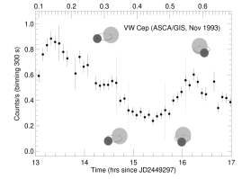
The first case reported in the literature of an eclipse of a flare in X-rays was an event in VW Cep (G5V/K0V), a binary system of the W UMa-type. These are eclipsing binaries that consist in F-K main sequence stars with short orbital periods. They are, in general, strong X-ray sources. The observed X-ray emission is attributed to magnetic activity caused by a dynamo. VW Cep is an unusual system, since the primary star (the deepest eclipse, at orbital phase $\phi$=0, occurs when this star is occulted, with $i=65\leavevmode\nobreak\ \degr$) is the hotter (G5V) but the less massive star ($M=0.25\,M_{\odot}$, $R=0.50\,R_{\odot}$), while the secondary (K0V, $M=0.90\,M_{\odot}$, $R=0.93\,R_{\odot}$) is more massive (see Hill 1989; Choi & Dotani 1998, and references therein). Choi & Dotani (1998) analyzed the ASCA light curve of VW Cep proposing that the observed dip during the decay of a flare, at $\phi\sim 0.42$ (Fig. 1), was produced by the eclipse of this flare. From investigation of the light curve they also conclude that the flare took place in the polar region of the most massive star (the K0V).

Figure 1: VW Cep X-ray light curve (ASCA/SIS and ASCA/GIS) in Feb. 2002. The solid lines mark the times of the optical eclipses. An eclipse in the flare, around $\phi\sim 0.45$, is displayed in the lower panel, where dotted lines indicate the phases of the four contacts used in the analysis, with a representation of the relative postions of the stars next to them.

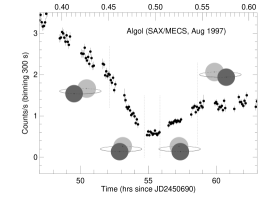
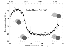
Algol (B8V/K2III) is an interesting target to search for eclipses ($i=82.5\leavevmode\nobreak\ \degr$) in X-rays, since the hot component of the system can be safely assumed to be dark in X-rays as compared to the K2III secondary, which is expected to host coronal features. Two eclipsed flares have been reported in Algol. Schmitt & Favata (1999) observed, in 1997, an eclipse with Beppo-SAX during the decay of a large flare. They estimated that the flare reached a maximum of 0.6 $R_{*}$ above the stellar surface, in a polar region in order to produce the observed eclipse centered around $\phi\simeq 0.50$, and a density of at least $\sim 10^{11}$ cm^-3 was necessary. Schmitt et al. (2003) reported another eclipse during a flare in Algol, observed with XMM-Newton in 2001, and they used a reconstruction method to conclude that the flare had a height of $\sim 0.1R_{*}$ (0.3 $R_{\odot}$) over the surface ($R_{1,2}=3.09/3.29R_{\odot}$), placed near the limb, with a density above $\sim 10^{11}$ cm^-3.

Figure 2: Algol light curve (BeppoSAX/MECS) in Aug 1997. An eclipse in the flare, around $\phi\sim 0.5$, is enlarged in the lower panel.

In this work we apply the same technique already used with SV Cam (Paper I) to the three cases mentioned above. In the case of VW Cep and the XMM observation of Algol we reanalyzed the data to calculate the phases of the four contacts. The paper is structured as follows: in Sect. 2 we describe the technical details of the observations; Sect. 3 develops the geometrical formulae used in this technique and the results found for each case. The results and their implications in the coronal context are discussed in Sect. 4, and the conclusions are given in Sect. 5.

2 Observations

VW Cep (HD 197433) was observed with ASCA on 5 Nov. 1993 23:37 UT (Choi & Dotani 1998). The ASCA satellite has four telescopes equipped with two Solid-State Imaging Spectrometers (SIS0, SIS1, range 0.4–10 keV), and two Gas Imaging Spectrometers (GIS2, GIS3, range 0.8–10 keV). We have reanalyzed the light curves by selecting a circular region around VW Cep, and subtracting the background level. The light curve displayed in Fig. 1 has been obtained by correcting for small time shifts between the two GIS datasets and then summing the signal. Times corresponding to the four contacts were determined in the GIS summed light curve.

Figure 3: Algol light curve (EPIC/PN) in Feb 2002. The optical eclipse takes place between $\phi\sim 0.43$ and $\phi\sim 0.57$. The eclipse in the flare, around $\phi\sim 0.54$, is displayed in the lower panel.

Two observations of Algol ($\beta$ Per, HD 19356, HR 936) are analyzed in this work. Algol was observed on 30 Aug. 1997 3:04 UT with BeppoSAX (Schmitt & Favata 1999). We use in this case the phases of the four contacts as provided by the authors. The corresponding light curve (Fig. 2), was constructed summing the data from all the three Medium Energy Concentrator Spectrometer (MECS) detectors (range 0.1-10 keV).

XMM-Newton observed Algol on 12 Feb. 2002 4:42 UT (Schmitt et al. 2003). The light curve used for the analysis is based on EPIC-PN (range 0.15-15 keV) data that we reanalyzed using the standard SAS (Science Analysis Software) version 6.1. We determined the four contacts of the eclipse as displayed in Fig. 3.

3 Results

In Paper I we made an analysis of an eclipse of a flare in SV Cam. In that case the high inclination ($i\sim 90\degr$) of the system simplifies the equations. Here we calculate new equations for the general case $i\neq 90\degr$. We assume that the emitting region has a spherical shape, and is defined by the following quantities: latitude ($\theta$), longitude ($\lambda$, with origin 0 the meridian of each star that is in front of the observer at $\phi$=0), height over the center of the star ($h$) and the radius of the spherical emitting region ($R_{3}$). We have made a grid of values for the 4 variables, and we then calculated the times when the four contacts of the eclipse take place for each set of values. We considered as valid results those that agree within 1 time bin (300 s for VW Cep and the Algol XMM observation, 600 s for Algol with BeppoSAX) with the measured times. We describe here the equations corresponding to a system with a primary star that hosts a flare which is eclipsed by the secondary. For the simple case (system with $i=90\degr$):

$$x^{\prime}_{1} = -a\sin(\phi),\quad y^{\prime}_{1}=0,\quad z^{\prime}_{1}=-a\cos{\phi}$$

$$x^{\prime}_{2} = -x^{\prime}_{1},\quad y^{\prime}_{2}=0,\quad z^{\prime}_{2}=-z^{\prime}_{1}$$

$$x^{\prime}_{3} = x^{\prime}_{1}+h\cos(\theta)\sin(\phi+\lambda),\quad y^{\prime}_{3}=y^{\prime}_{1}+h\sin(\theta),\quad$$

$$z^{\prime}_{3} = z^{\prime}_{1}+h\cos(\theta)\cos(\phi+\lambda)$$

where $x^{\prime}$, $y^{\prime}$ correspond to the coordinates in the plane in front of the observer (Fig. 4), $z^{\prime}$ is the coordinate of the axis perpendicular to this plane (positive towards the observer), and $a$ is the value of the semi-axis of the orbit. $x^{\prime}_{3}$, $y^{\prime}_{3}$, $z^{\prime}_{3}$ correspond to the position of the emitting region of the flare, and the subindices 1 and 2 correspond to the positions of the centers of the primary and secondary stars respectively.

Figure 4: Schematic view of the geometry of the stars and the flaring region (dashed) at phase $\phi\sim 0.15$.

Now, for the general case in which $i\neq 90\degr$ we need to apply a rotation. In the new coordinates system, $x,y,z$ can be calculated from the former coordinates:

$$x=x^{\prime},\quad y=\sin i\,y^{\prime}-\cos i\,z^{\prime},\quad z=\cos i\,y^{\prime}+\sin i\,z^{\prime}$$

and therefore,

$$x_{1} = -a\sin\phi,\quad y_{1}=a\cos\phi\cos i,\quad z_{1}=-a\cos{\phi}\sin i$$

$$x_{2} = a\sin\phi,\quad y_{2}=-a\cos\phi\cos i,\quad z_{2}=a\cos{\phi}\sin i$$

$$x_{3} = x_{1}+h\cos\theta\sin(\phi+\lambda),\quad$$

$$y_{3} = y_{1}+h[\sin\theta\sin i-\cos\theta\cos(\phi+\lambda)\cos i]$$

$$z_{3} = z_{1}+h[\sin\theta\cos i+\cos\theta\cos(\phi+\lambda)\sin i]$$

Table 1: VW Cep (G5V/K0V, $R_{1,2}$=0.50/0.93 R_⊙) range of possible solutions of the eclipse of a flare in 1993.

Flaring star	Ecl. star	$\theta$($\degr$)	$\lambda$($\degr$)	$h$ (R⊙)	$h-R_{*}$ (R∗)	$R_{3}$ (R⊙)	$\log n_{\rm e}$ (cm-3)	$B$ (G)
Sec	Pri	$+12.5-+14.3$	173.3–176.2	1.53–1.66	0.65–0.78	0.002–0.012	12.8–14.0	800–3300
Sec	Sec	$-17.5-+49.0$	20.8–25.2	0.95–1.87	0.02–1.01	0.010–0.273	10.7–12.9	76–910
“	“	$-49.9--39.1$	20.8–25.2	1.63–1.87	0.75–1.01	0.084–0.223	10.9–11.5	88–180
Sec	S+P	$-52.7--42.9$	20.8–25.2	1.62–1.87	0.74–1.01	0.084–0.197	11.0–11.5	98–180
Pri	Pri	$+37.5-+55.0$	20.7–25.2	0.50–0.54	0.00–0.08	0.002–0.014	12.7–14.0	710–3000
All results		$-53-+55$	20.7–25.2 or 175	0.50–1.87	0.00–1.01	0.002–0.273	10.7–14.0	76–3300

Figure 5: Relative positions of the VW Cep stars (dashed lines) during first contact ($\phi$=0.337), as seen from the front (left panel) and top (right panel). All the possible results are represented with black points indicating the center of the emitting region. A dotted line marks the equator (left panel) and the meridian origin of longitude (both panels). Longitude goes positive counter-clockwise.

At the first and fourth contacts the distance between the center of the flare and the center of secondary star must be:

$$\Delta_{1}=\sqrt{(R_{2}+R_{3})^{2}-(y_{3}-y_{2})^{2}}$$

and similarly, at the second and third contact:

$$\Delta_{2}=\sqrt{(R_{2}-R_{3})^{2}-(y_{3}-y_{2})^{2}}$$

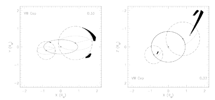
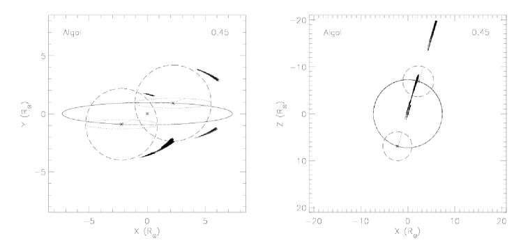
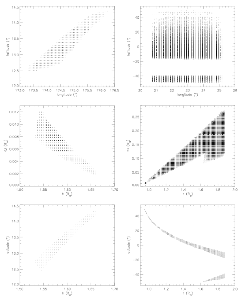
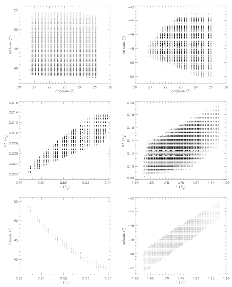
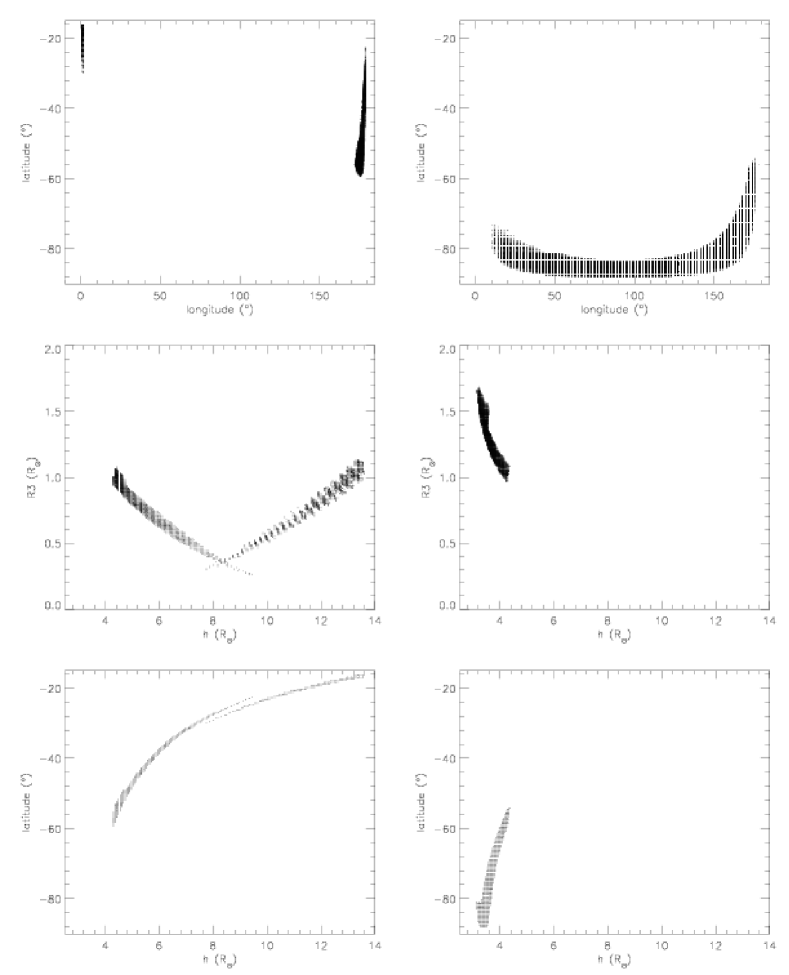
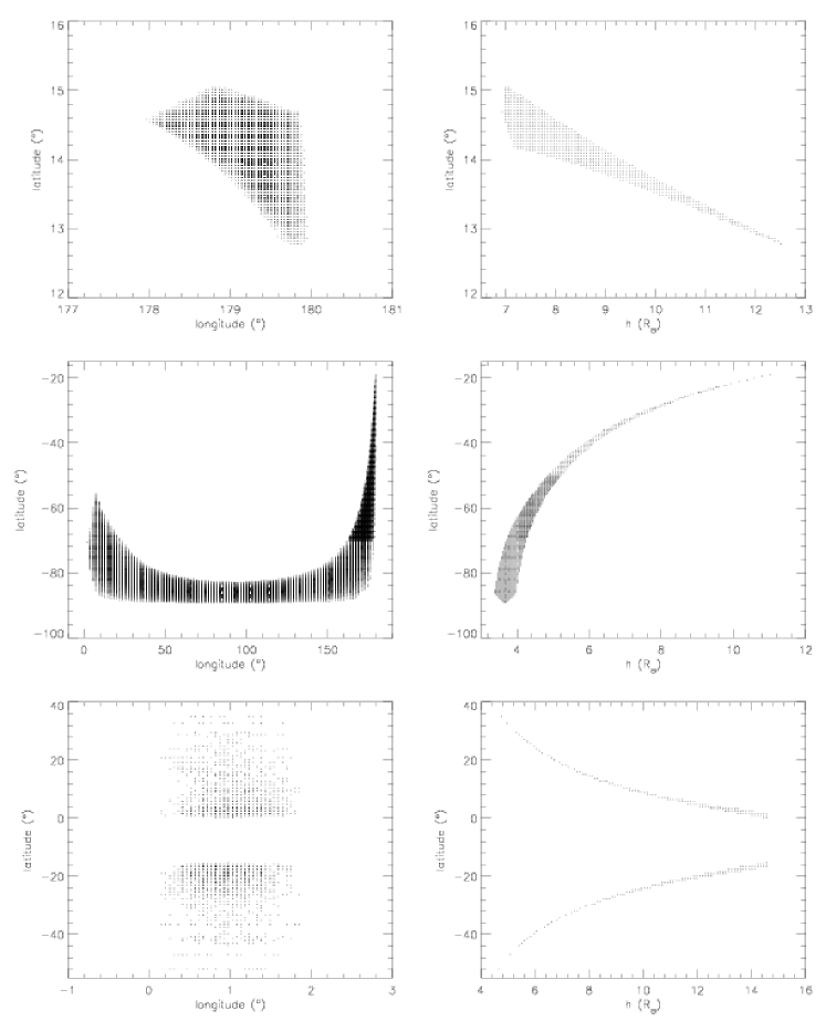
Thus, we will have four equations: $x_{3}=x_{2}+\Delta_{1},\quad x_{3}=x_{2}+\Delta_{2},\quad x_{3}=x_{2}-\Delta_{2},\quad x_{3}=x_{2}-\Delta_{1}$ that we can use to calculate numerically the times of the four contacts for each point of the grid. Similar equations can be easily derived for the other configurations of the flare. Some geometrical constraints can be added to ensure the totality of the eclipse ($y_{3}+R_{3}\leq y_{2}+R_{2}$) and a valid position in $z$ ($z_{3}+\Delta_{1}<z_{2}$). In cases with large values of $h$ we have imposed another constraint: the centrifugal force must be lower than the resulting gravitational forces of the two stars. In this way, $h+R_{3}$ must be lower than a certain value that is very close to $a$. Further restrictions can be imposed regarding the light curve observed during the phases in which no eclipses where observed: $(x_{3}-x_{2})^{2}+(y_{3}-y_{2})^{2}>R_{2}+R_{3}$ (substitute the subindex $2$ with $1$ to avoid eclipses by the primary). The results found are shown in Tables 1, 2 and in Figs. 5–7. More detailed results are found in Figs. 8-11, and Fig. 12 show several animations of valid solutions in the three flares.

The physical interpretation of an emitting region shaped as a sphere detached from the surface could be the apex of the loops involved in the flare, with the emitting region being the place of magnetic reconnection. Although the real shape is unlikely to be a sphere, such a form is the simplest approximation and would be the smallest sphere that contains the real emitting region. We have also conducted a test using the shape of a loop (see Sect. 3.4 and Sect. 4), and another test considering only the central points of the eclipse (See Sect. 4), yielding similar results. We therefore conclude that the use of a sphere gives valid results.

An additional result can be obtained from the temperature ($T$) and emission measure (EM) of the flare. We can calculate the electron density ($n_{\rm e}$) of the emitting region by calculating the EM during the flare. In this case we use the values of the $T$ and EM determined in the original papers when available. Since EM$\sim 0.8\,n_{\rm e}^{2}\,V$, it is possible to get the density $n_{\rm e}$ from the net flare EM, using $V=4/3\pi R_{3}^{3}$. If we consider that the magnetic pressure, $B^{2}/(8\pi)$, should be at least as large as the electron pressure ($2n_{e}kT$), we can get the minimum magnetic field needed to have a stable structure in the flare. In the cases in which the whole sphere of the flaring region is not observable, we have corrected the volume $V$ by a factor accounting for the visible fraction. The results of the $n_{\rm e}$ and $B$ are listed in Tables 1–2. Next we describe the particular details of each of the three eclipses.

Table 2: Algol (B8V/K2III, $R_{1,2}$=3.09/3.29 R_⊙) range of possible solutions of the eclipses of the flares in 1997 and 2002.

Observation	$\theta$($\degr$)	$\lambda$($\degr$)	$h$ (R⊙)	$h-R_{2}$ (R∗)	$R_{3}$ (R⊙)	$\log n_{\rm e}$ (cm-3)	$B$ (G)
BeppoSAX	$+12.7-+13.9$	178.6–179.8	7.81–12.5	1.37–2.80	0.033–0.33	11.8–13.3	630–3500
“	$-87.98--22.5$	10.10–179.2	3.14–9.45	$-0.05$ – +1.87	0.26–1.69	10.8–11.9	220–750
BeppoSAX (self-eclipsed)	$+1.0-+15.6$	0.4–1.6	7.50–13.60	1.28–3.13	0.29–1.19	10.9–11.8	240–690
“	$-30.0--16.4$	0.4–1.6	7.75–13.60	1.36–3.13	0.30–1.13	11.0–11.80	250–670
XMM-Newton	$+6.9-+16.0$	197–272	3.75–7.31	0.14–1.22	0.078–0.31	11.0–11.9	150–420
“	$-50.5--24.8$	198–323	5.82–10.7	0.77–2.25	0.093–0.76	10.4–11.8	76–370

Figure 6: Relative positions of the Algol stars (dashed lines) during first contact ($\phi$=0.451) in the Beppo/SAX observations, as seen from the front (left panel) and top (right panel). All the possible results are represented with black points indicating the center of the emitting region.

3.1 VW Cep

The eclipse detected in VW Cep with ASCA was analyzed by Choi & Dotani (1998). They concluded that the dip observed in the light curve (see Fig. 1) corresponds to an eclipse of the flaring region. Since the decay of the flare lasts almost one orbital period, they assume that the flare must occur in a polar region because otherwise it would be occulted by one of the stars out of the eclipse. Therefore Choi & Dotani (1998) conclude that the flare occur in a polar region of the primary. They calculate also the size scale of the flare from the ingress and egress times yielding a size of $\sim 5.5\times 10^{10}$ cm ($\sim 0.8R_{\odot}$), ignoring the rotational velocity of the secondary star because the flare is assumed to be polar. Rotational modulation will however be produced only if the emitting region of the flare is close enough to the stellar photosphere to be occulted.

We have reanalyzed the data, and determined that the phases of the four contacts are $\phi$=0.337, 0.374, 0.486 and 0.548 respectively, using the elements provided by Aluigi et al. (1994), where $P_{\rm orb}$=0.2783076 and $T_{0}$=2,448,862.5220 (at $\phi$=0 the G5V star is behind the K0V star), and the stellar data given by Hill (1989). If we assume that the dip observed corresponds to an eclipse (rather than the decay of a flare followed by a second flare), then this eclipse partially overlaps with the secondary optical eclipse, and therefore it is likely that a flare in the secondary is eclipsed by the primary. We have considered also the cases in which the flare is self-eclipsed by the host star. If the emitting region is a flare in the primary separated from the stellar surface, it is not possible to distinguish it from a flare in the secondary occulted by the primary. The results of the analysis (displayed in Fig. 5 and Table 1) indicate that no flare in polar regions ($|\theta|>55\degr$) can produce the observed light curve, and that the flare could be either associated with the primary or the secondary. Besides, the size of the emitting region is always $R_{3}<0.3$ R_⊙, well below the calculations of Choi & Dotani (1998).

We have calculated the electron density based on the EM during the flare. We have used the same values calculated by Choi & Dotani (1998): $\log T_{1,2}=6.87,7.35$ (K) and $\log EM_{1,2}=52.56,52.58$ (cm^-3). Results are displayed in Table 1.

Although the SIS and GIS light curves are suggestive of an eclipse of a flare, we cannot reject the possibility that there are actually two flares. However we believe that the slight increase in the slope at the “first contact” might be an indication of an eclipse rather than a fast decay of a first flare (the SIS light curve seemed to indicate more clearly the eclipse interpretation, see Choi & Dotani 1998).

3.2 Algol with BeppoSAX

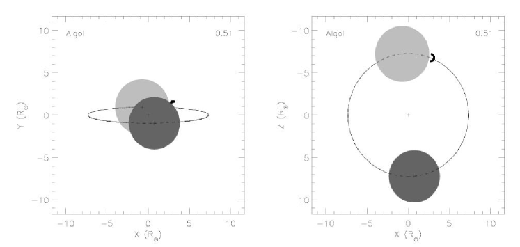
BeppoSaX detected a very remarkable flare in Algol in 1997, with an increase in X-ray flux by 2 orders of magnitude. Besides, the flare was eclipsed during the decay in a rather clean light curve. Schmitt & Favata (1999) analyzed these data, and they concluded that the flaring region was placed near the southern pole. If we apply our method to the same data (using the same phases calculated by Schmitt & Favata 1999), we have a set of results in a wide range of latitudes, and even some at $\theta\sim 15.6\degr$ in the northern hemisphere. Among the results found, those in the northern hemisphere with the flare eclipsed by the primary imply a relatively large distance from the secondary star ($h$), and such positions are likely hampered by gravitational forces of the secondary star and/or some mass transfer given the low latitude and short distance of these solutions to the center of mass of the system. However we did not compute the effects of gravity in order to reject these solutions. Another set of results in the southern hemisphere indicates that the flaring region could still be present at latitudes between $-22$ and $-59\degr$, in this case at lower heights over the secondary, and likely less affected by mass transfer processes. Finally, those results related to a self-eclipse by the secondary star imply large values of $h$ and low latitudes, but no mass transfer can be involved in this case (see Table 2).

Figure 7: Relative positions of the Algol stars (dashed lines) during first contact ($\phi$=0.516) in the XMM observations, as seen from the front (left panel) and top (right panel). All the possible results are represented with black points indicating the center of the emitting region.

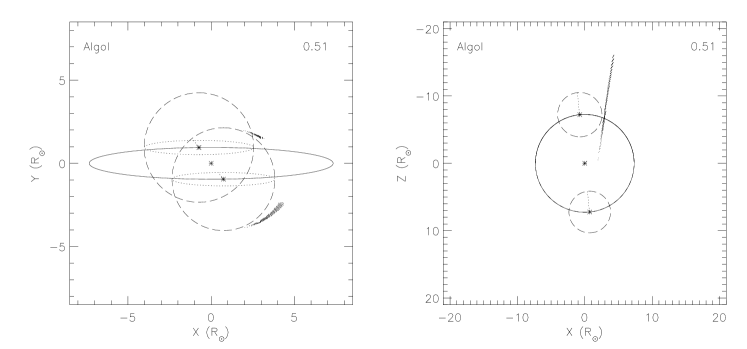
The phases of the eclipse (0.451, 0.488, 0.505, 0.545) make this analysis more complicated than the others. While in the other cases the range of solutions does not depend on the approximation of a spheric shape for the emitting region, in this particular case (totality happens while there is a stellar conjunction) it is possible to find other solutions consisting in an eclipse of a flare that is very close to the surface. In order to model this case we assumed that a sphere partially below the photosphere of the star might produce the same light curve, and therefore we have relaxed the conditions to allow this geometry to happen. This workaround allows us the use of spheric caps in the analysis as well. This situation is not considered for the other two eclipses (VW Cep and Algol with XMM-Newton) because the geometry of the eclipses is not compatible with this configuration: the Algol case is explained below, and the second contact of the coronal eclipse of VW Cep occurs when the photospheric eclipse starts (see Fig. 2), and therefore only a region detached from the surface can be totally eclipsed at that time. The electron density under this configuration has been calculated using the volume of the emitting region that is visible (note that in some cases the emitting region is partially occulted below the secondary star during the whole flare). The solutions found under this configuration show that the flare could be present at almost any longitude near the south pole of the star, producing the same kind of light curve eclipse as the other results mentioned in former paragraph.

3.3 Algol with XMM-Newton

XMM-Newton detected a flare in Algol in 2002 that was analyzed by Schmitt et al. (2003), who concluded that an eclipse of the flare was taking place, indicating that the flare should have occurred near the limb in the northern hemisphere since the first contact takes place at $\phi>$0.5. In this case Schmitt et al. (2003) used a reconstruction of the flaring plasma region using the whole light curve, concluding that the flare takes place at a height of $\sim 0.1R_{*}$ ($R_{2}=3.29R_{\odot}$) and $\theta<69\degr$.

We have determined the phases of the four contacts at 0.516, 0.527, 0.554, 0.565 using the ephemeris of Al-Naimiy et al. (1985), where $P_{\rm orb}$=2.8673285 d and $T_{0}$=2,445,739.003. These values are in agreement with those proposed by Schmitt et al. (2003), although they only expressed the first three contacts and assumed that the fourth contact takes place at the end of the observation. We do not expect this to affect the range of solutions. However there is an alternative interpretation of the light curve: the eclipse could actually be starting at phase 0.506 (the apparent peak of the flare), while the change in slope at $\phi\sim 0.516$ could actually correspond to the flare maximum emission. The determination of the fourth contact has also some uncertainty. The analysis of the light curves of different energy bands (Schmitt et al. 2003) seems to suggest that the eclipse following a flare maximum is the best option, so we will refer to this situation from now on.

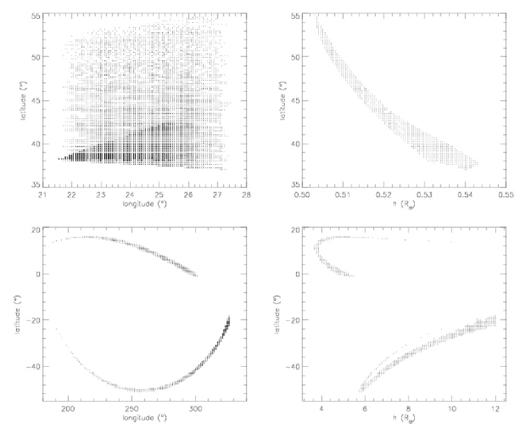
Given the phases involved in the eclipse (see Fig. 3) it is easier to analyze this flare than the BeppoSAX flare, since a configuration of an emitting region overlapping with the star is not possible: the eclipse starts after $\phi\sim 0.5$, invalidating the solutions in the southern hemisphere, and those in the northern hemisphere were rejected in the analysis. We only found valid solutions for the configuration in which the flare (hosted by the secondary) is eclipsed by the primary star. Solutions, including the result reported by Schmitt et al. (2003), are possible both in the northern ($7\degr\la\theta\la 16\degr$) and southern hemisphere ($-50\degr\la\theta\la-25\degr$), and given the position of the flare (Figs. 7, 11) in most cases it is unlikely that the flaring region is affected by the mass transfer between the two stars.

Since Schmitt et al. (2003) do not report the value of the EM, we made a spectral fit to the spectrum in the quiescent emission (log EM [cm^-3]=53.64) and in the flaring non-eclipsed emission (log EM [cm^-3]=53.89), resulting in a net value for the flare of log EM [cm^-3]=53.53 at log $T$ [K]$=7.50$. The range of possible values of the electron density (Table 2) are consistent with those reported by Schmitt et al. (2003), but unlike Schmitt et al. (2003) we also found solutions in the southern hemisphere, and a wider range of solutions in the northern hemisphere.

8

Figure 8: Results of the flare in VW Cep, flare in the secondary. Left: eclipsed by primary. Right: self-eclipsed by secondary.

9

Figure 9: Results of the flare in VW Cep. Left: flare in primary, self-eclipsed by primary. Right: flare in secondary, the eclipse starts behind secondary and ends behind the primary.

10

Figure 10: Results of the flare in Algol observed with BeppoSAX, solutions in the southern hemisphere. Left: The emitting region is detached from the surface of the star (the results around $\lambda\sim 1\degr$ correspond to self-eclipse by the secondary). Right: The emitting region can overlap with the star (therefore it can be a spheric cap).

11

Figure 11: Results of the flare in Algol. Left: Observed with BeppoSAX, solutions in the northern hemisphere (the results around $\lambda\sim 1\degr$ correspond to self-eclipse by the secondary). Right: Observed with XMM-Newton.

12

Figure 12: Several examples of animations of valid results with different configurations. A white circle (or loop) indicates the emitting region of the flare being eclipsed. The latitude and longitude used in the simulations are shown in the upper panel, while the light curve is displayed in the lower panel.

Figure 13: Schematic view of the coronal loop. The loop lies around the XZ plane. The Z axis points opposite from the center of the host star and Y axis is paralel to the closest meridian.

3.4 Eclipses of coronal loops

The shape chosen for the analysis has been the simplest possible, a sphere. The use of a different geometry will further restrict the number of solutions. Since there is an infinite range of shapes possible, we have chosen only one particular case to show the deviation from the solutions found with the sphere. We chose a shape similar to what is observed in solar coronal loops. Following the notation used in the paper we have defined a torus contained in a sphere of radius $R_{3}$ (the external radius of the torus), a cross-section radius fixed to $R_{4}=0.2\,R_{3}$, and a circular curvature. The arc is placed perpendicular to the stellar surface (see Fig. 13), with a local reference frame with the Z axis pointing opposite from the center of the star and the Y axis parallel to the tangent of the nearest meridian. In this local reference frame we can define each of the points ($x_{\rm i},y_{\rm i},z_{\rm i}$) of the loop using two angles ($\beta$, $\delta$) and a radial variable ($r$, the radius of the cross-section) as follows:

$$x_{\rm i} = (R_{3}-R_{4}+r\cos\,\delta)\cos\,\beta,\quad y_{\rm i}=r\sin\,\delta,$$

$$z_{\rm i} = (R_{3}-R_{4}+r\cos\,\delta)\sin\,\beta$$

where r varies from 0 to $R_{4}$, $\beta$ from 0$\degr$ to 180$\degr$ and $\delta$ from 0$\degr$ to 360$\degr$. In order to account for the eclipses coverage we need to transform the local coordinates ($x_{\rm i},y_{\rm i},z_{\rm i}$) into the coordinates of the rest reference frame used for the stellar system (Fig. 4). We need to apply 3 rotations, in latitude ($\theta$), in longitude ($\lambda+\phi$), and in inclination ($i$):

a rotation in latitude (around X),

$$x^{\prime}=x,\quad y^{\prime}=(\cos\,\theta)\,y+(\sin\,\theta)\,z,\quad z^{\prime}=(-\sin\,\theta)\,y+(\cos\,\theta)\,z,$$

a rotation in longitude (around Y),

$$x^{\prime\prime} = \cos(\phi+\lambda)\,x^{\prime}+\sin(\phi+\lambda)\,z^{\prime},\quad y^{\prime\prime}=\,y^{\prime},$$

$$z^{\prime\prime} = -\sin(\phi+\lambda)\,x^{\prime}+\cos(\phi+\lambda)\,z^{\prime},$$

and a rotation due to inclination (around X),

$$x^{\prime\prime\prime} = x^{\prime\prime},\quad y^{\prime\prime\prime}=(\sin\,i)\,y^{\prime\prime}-(\cos\,i)\,z^{\prime\prime},$$

$$z^{\prime\prime\prime} = (\cos\,i)\,y^{\prime\prime}+(\sin\,i)\,z^{\prime\prime},$$

Therefore, the position of a point of the loop in the same reference frame used in the problem will be:

$$x^{\prime\prime\prime}_{\rm i} = x_{3}+\cos(\phi+\lambda)\,x_{\rm i}+\sin(\phi+\lambda)\,(-\sin\,\theta\,y_{\rm i}+\cos\,\theta\,z_{\rm i}),$$

$$y^{\prime\prime\prime}_{\rm i} = y_{3}+\sin\,i\,(\cos\,\theta\,y_{\rm i}+\sin\,\theta\,z_{\rm i})-\cos\,i\,(-\sin(\phi+\lambda)\,x_{\rm i}+$$

$$\cos(\phi+\lambda)\,(-\sin\,\theta\,y_{\rm i}+\cos\,\theta\,z_{\rm i}),$$

$$z^{\prime\prime\prime}_{\rm i} = z_{3}+\cos\,i\,(\cos\,\theta\,y_{\rm i}+\sin\,\theta\,z_{\rm i})+\sin\,i\,(-\sin(\phi+\lambda)\,x_{\rm i}+$$

$$\cos(\phi+\lambda)\,(-\sin\,\theta\,y_{\rm i}+\cos\,\theta\,z_{\rm i}),$$

We have applied this method to search for the results in the case of the flare observed with XMM-Newton in Algol. In Fig. 14 we display a valid solution near the equator, with a simulation included in Fig. 12. The possible solutions (Fig. 15) are very similar to those found for a spheric shape (the $h$ and $R_{3}$ are slightly different since $R_{3}$ has a different definition). The density derived from this geometry would also be higher than that derived from the spheric case.

Figure 14: An example of a valid solution using a coronal loop placed at $\theta=10.1\degr$, $\lambda=258.2\degr$, $R_{3}=0.53\,{\rm R}_{\odot}$ and $h=3.52\,{\rm R}_{\odot}$. Views from the front (left panel) and the top (right panel) during first contact.

15

Figure 15: Range of valid solutions for the case of a coronal loop in the XMM-Newton flare with the proposed orentation. Flare happens in secondary, and it is eclipsed by primary.

4 Discussion

The approach presented here constrains the geometry (location and size) of the flaring region for eclipsed flares. A simple calculation also yields a lower limit of the electron density (the plasma does not need to be homogeneously distributed in a sphere). The results are consistent with the range of values derived from density-sensitive line ratios in active stars. The method assumes that the emission measure remains constant during the eclipse (this is important only for the calculation of electron density and magnetic field), and that the spherical shape of the emitting region remains unchanged during the eclipse. This shape has been chosen as the simplest possible approximating a compact region. Spheres with a filling factor lower than 1 would imply higher values of the electron density, and we do not expect that other shapes vary substantially the results of latitude, longitude and height, except in cases like the BeppoSAX Algol flare, where the flaring region can be actually attached to the surface and have a significant surface filling factor. The solutions where the emitting region is detached from the surface could correspond to the apex of the loops involved in the flare, although magnetic reconnection in the solar flares does not happen necessarily at the apex, and the site of reconnection does not need to be the site of maximum X-ray emissivity. Although it is unlikely that the emitting region is a sphere, we consider this a good approximation in order to search for the location. We have conducted two tests to quantify the relevance of the shape chosen with respect to the real solutions. A first test was conducted using a coronal loop instead of a sphere (see Sect. 3.4), and considering the four contacts of the eclipse. The orientation of the loop (with the shape of a torus) was fixed, as well as the cross-section radius (0.2  $R_{3}$). The set of results is similar to that of spherical shape, but the range of solutions is smaller. In the second test, we have considered the simpler case in which only two contacts are used in the model. These contacts would correspond to the ingress (midpoint between $\phi_{1}$ and $\phi_{2}$) and egress (midpoint between $\phi_{3}$ and $\phi_{4}$) of the center of the emitting region, and therefore independent of its shape. The test conducted has shown that the range of solutions is similar to those obtained for the restrictions imposed by the use of four contacts and a spherical shape. The results are displayed in Figs. 16–18. These two tests confirms that the approximation of a sphere can be valid also as an approximation for more complicated shapes.

16

Figure 16: Results obtained for the flare observed in Algol with BeppoSAX for the simpler case of two contacts only (ingress and egress of the center of the emitting region). From top to bottom: solutions in the northern hemisphere (flare in the secondary eclipsed by the primary), solutions in the southern hemisphere, and solutions for the case of eclipse of the flare by the secondary star itself.

17

Figure 17: Results for the case of two contacts only in VW Cep. From top to bottom: flare in secondary eclipsed by primary, self-eclipsed by secondary only, and eclipse starting behind secondary and ending behind primary.

18

Figure 18: Results for the case of two contacts only. Upper panels: VW Cep, self-eclipsed by primary. Lower panels: eclipse in Algol observed by XMM (flare in secondary, eclipsed by primary).

While the original analyses of these events pointed towards polar flares, (Choi & Dotani 1998; Schmitt & Favata 1999), this work has shown that other configurations are possible from the geometric point of view. A polar location is only possible for the Algol flare observed with BeppoSAX. In this work we do not privilege any solution among the possible results, and consider all configurations as equally possible as long as they do not violate any physical law. Gravity forces or mass transfer between close binaries should be considered in order to constrain the number of solutions.

The analysis poses a clear lower limit in electron density of $\log n_{e}$ (cm^-3)=10.4, well in agreement with the minimum values determined from line ratios analysis in active stars. The largest values compatible with the geometrical configurations, specially those with $\log n_{e}$ (cm^-3) $\ga 13$, are larger than those commonly observed in the X-ray line ratios of most stars (e.g. Sanz-Forcada et al. 2003; Testa et al. 2004; Ness et al. 2004). The measurements of the size of the emitting region shows that although the emitting regions are small compared to the stellar size, we cannot reject large loop lengths (measured through the variable $h$) by applying only geometrical constrains based on the eclipse contacts.

5 Conclusions

We have systematically searched the solution space to calculate the geometrical characteristics of the emitting region of four flares in active stars. The method uses the times of the four contacts of the eclipse and simulates all possible geometrical situations assuming that the emitting region has a spherical shape and no substantial geometrical changes during the eclipse. Two tests (including the use of a loop) were conducted to prove that the approximation of a spherical shape is appropriate, even if the real shape is not a sphere. The solutions found in the three flares analyzed in this work and that of Paper I show that polar flares are not possible in three of the four flares, and electron densities must be larger than $\log n_{e}$ (cm^-3)=10.4, consistent with measurements from line ratios of density sensitive lines in active stars. The magnetic fields needed to confine these loops range in both systems between 75 G and 3300 G. The emitting regions have sizes that range from 0.002 to 0.5 $R_{*}$, and they can be at a distance (interpreted as loop length) of up to 3.1 $R_{*}$ from the star’s surface. Further refinement based on other physical limitations, such as gravity or mass transfer could further constrain the set of solutions.