Magnetic Coupling of a Rotating Black Hole with Advection-Dominated Accretion Flows

Abstract

A model of magnetic coupling (MC) of a rotating black hole (BH) with advection-dominated accretion flow (MCADAF) is proposed. It turns out that MCADAF providers a natural explanation for the transition radius between ADAF and SSD, and could be used to interpret the highest luminosity of GX 339-4 in hard-state. A very steep emissivity index can be produced in the innermost part of the MCADAF, which is consistent with the recent XMM-Newton observations of the nearby bright Seyfert 1 galaxy MCG-6-30-15 and with two X-ray binaries (XRBs): XTE J1655-500 and GX 339-4. In addition, we estimate the BH spins in Seyfert 1 galaxy MCG-6-30-15 and in the two XRBs based on this model.

and

1 INTRODUCTION

More than three decades ago, the standard thin disk was proposed by Shakura & Sunyayev (1973, hereafter SSD), which is regarded as the milestone of black hole (BH) accretion theory. However, the effective radiation temperature is very low in SSD, being obviously not consistent with the observations of the hard X-ray and gamma-ray radiation in X-ray binaries (XRBs). In order to overcome this shortcoming, some authors proposed the cooling-dominated hot disk (Shapiro, Lightman & Eardley 1976, hereafter SLE). A vital disadvantage with SLE lies in thermal instability. Not long ago, advection-dominated accretion flow (hereafter ADAF) was suggested by some authors (Narayan & Yi 1994, hereafter NY94; 1995a; 1995b; Abramowicz 1995; Esin 1997; Manmoto 1997; Gammie and Popham 1998; Popham and Gammie 1998; Yuan 1999). The ADAF model succeeds in explaining the observed spectra of some sources, such as Sgr A* (Narayan 1995c), NGC4258 (Lasota 1996) and GRO J1655-40 (Lasota 1998). Recently, Yuan (2001 hereafter Y01; 2003) extended the ADAF model and put forward a new two-temperature hot branch of equilibrium solutions, i.e., the luminous hot accretion flow (hereafter LHAF). It is argued in Y01 that LHAF is much more luminous than ADAF as the entropy of the accreting mater supply the radiation as well as the viscous dissipation.

Yuan (2006, hereafter Y06) pointed out that the hard states at their highest luminosities of some XRBs could not be explained by ADAF, while LHAF can produce the highest luminosity in the hard state of XTE J1550-564. However, as argued in Y06 that neither ADAF nor LHAF could be used to explain the highest luminosity of GX 339-4 (Done & Gierlinski 2003; Zdziarski et al. 2004), which is a great challenge to LHAF. Probably, an efficient way of increasing the luminosity in hard-state is the magnetic coupling (MC) process, which is an important mechanism for extracting energy from a rotating BH (Blandford 1999; Li & Paczynski 2000; Li 2002a, hereafter L02; Wang et al. 2002, 2003, hereafter W02, W03, respectively). However, the MC has been formulated in the context of a relativistic thin disk (henceforth MCTHIN, Page & Thorne 1974; L02; W03), in which both the gravitational energy of the accreting matter and the rotational energy transferred into the disk are assumed to be radiated away in black-body spectrum. Thus MCTHIN is obviously not consistent with observed hard power-law X-ray spectra.

To solve the above puzzle in LHAF we intend to incorporate the MC with ADAF (henceforth MCADAF). It turns out that the steep emissivity index in Seyfert 1 galaxy MCG-6-30-15 and the two XRBs: XTE J1655-500 and GX 339-4 could be interpreted based on MCADAF, and our fittings are consistent with the low BH spins in these sources, and that the observation of the highest hard-state luminosity of GX 339-4 could be explained. Furthermore, a transition radius between ADAF and SSD could be given naturally in MCADAF with the hard X-rays spectra produced in the MC region.

This paper is organized as follows. In $\S$ 2 MCADAF is outlined, and the expressions of the MC power and torque in MCADAF are derived. In $\S$ 3, the MC effects on disk radiation and the emissivity index are discussed. It is found that the emissivity index is consistent with the recent XMM-Newton observations of the nearby bright Seyfert 1 galaxy MCG-6-30-15 and the two XRBs: XTE J1655-500 and GX 339-4 for the low BH spin. Finally, in $\S$ 4, we summarize our main results. Throughout this paper the geometric units $G=c=1$ are used.

2 DESCRIPTION OF MCADAF

In the previous MC model the disk is regarded as a thin disk, in which the rotational energy transferred from the BH to the inner disk is assumed to radiate away as the black body spectrum. In MCADAF, however, this assumption is changed to overcome the shortcomings of MCTHIN. It is assumed that only a fraction of energy transferred in the inner disk is radiated, and the rest energy deposited in the accreting matter as entropy is delivered to the BH as ADAF. Thus we have the magnetic field configuration of MCADAF as shown in Figure 1, in which ADAF is located in the MC region with closed field lines penetrating the accretion flow, and SSD is located outside the MC region. This configuration is significantly different from that given in W02 for MCTHIN, and a transition radius between ADAF and SSD is given naturally in MCADAF.

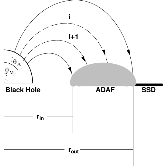
Figure 1: The poloidal magnetic field for MCADAF, in which ADAF and SSD are located inside and outside of $r_{out}$, respectively.

In order to facilitate the discussion on MCADAF in an analytic way, we make the following assumptions.

(i) ADAF is both stable and perfectly conducting, and the closed magnetic field lines are frozen in the accretion flow.

(ii) The magnetic field is assumed to be weak, and the instabilities of the magnetic field are ignored. The magnetosphere is stationary, axisymmetric and force-free outside the BH and ADAF.

Following Armitage & Natarajan (1999), the total pressure $P$ in the inner part of MCADAF is given by

$$P=\frac{\sqrt{2}\dot{M}}{12\pi\alpha_{{}_{S}}}(5+2{\varepsilon}^{\prime})^{1/2}(M/r^{5})^{1/2},$$ (1)

where the magnetic pressure $P_{mag}$ is related to the total pressure $P$ by

$$P_{mag}=B_{D}^{2}/8\pi=(1-\beta_{S})P.$$ (2)

In equations (1) and (2) $\alpha_{{}_{S}}$ is the viscosity parameter, $\beta_{S}$ is the ratio of gas pressure to total pressure, and ${\varepsilon}^{\prime}$ is defined as ${\varepsilon}^{\prime}=\varepsilon/f=\frac{5/3-\gamma}{f(\gamma-1)}$ (NY94). The parameter $f$ measures the degree to which the flow is advection-dominated, and $\gamma=\frac{8-3\beta_{S}}{6-3\beta_{S}}$ is the ratio of specific heats (Esin 1997). Thus we have

$${\varepsilon}^{\prime}=\frac{1-\beta_{S}}{f}.$$ (3)

Combining equations (1) and (2), we have the expression for the magnetic field in the inner part of the MCADAF as follows,

$$B_{D}=\sqrt{(2\sqrt{2}/3)(5+2{\varepsilon}^{\prime})^{1/2}\alpha_{{}_{S}}^{-1}(1-\beta_{S})M^{1/2}\dot{M}r^{-5/2}}.$$ (4)

Narayan et al. (1998) pointed out that the inner edge radius of an ADAF is located between $r_{mb}$ and $r_{ms}$, i.e.,

$$r_{mb}\leq r_{in}\leq r_{ms}.$$ (5)

where $r_{mb}$ and $r_{ms}$ are the radii of the innermost bound circular orbit and the last stable circular orbit, respectively. The radius $r_{in}$ can be expressed by

$$\left\{{\begin{array}[]{l}r_{in}\equiv M\chi_{in}^{2},\\ \chi_{in}=\chi_{mb}+\lambda(\chi_{ms}-\chi_{mb}),\end{array}}\right.$$ (6)

where $\chi_{mb}\equiv\sqrt{{r_{mb}}\mathord{\left/{\vphantom{{r_{mb}}M}}\right.\kern-1.2pt}M}$ and $\chi_{ms}\equiv\sqrt{{r_{ms}}\mathord{\left/{\vphantom{{r_{ms}}M}}\right.\kern-1.2pt}M}$. The parameter $\lambda$ is used to adjust the position of the inner edge of the ADAF, and $\lambda=0.5$ is adopted in calculations. Thus equation (4) can be expressed by

$$B_{D}\approx B_{0}C\xi^{-5/4},$$ (7)

$$B_{0}=M^{-1}\dot{M}^{1/2}=1.38\times 10^{9}m_{{}_{BH}}^{-1/2}\dot{m}^{1/2}Gauss,$$ (8)

$$C=(2\sqrt{2}/3)^{1/2}(5+2{\varepsilon}^{\prime})^{1/4}\alpha_{{}_{S}}^{-1/2}(1-\beta_{S})^{1/2}\chi_{in}^{-5/2},$$ (9)

   (a)

   (b)

Figure 2: The curves of $\lg[B_{D}(Gauss)]$ in MCADAF versus $\xi$ with $m_{{}_{BH}}=10$ for (a) $f$=0.5 and $a_{\ast}$= 0.3, 0.5 and 0.7 in solid, dotted and dashed lines, respectively, and for (b) $a_{\ast}$=0.5 and $f$= 0.3, 0.5 and 0.7 in solid, dotted and dashed lines, respectively.

where $\xi\equiv r\mathord{\left/{\vphantom{r{r_{in}}}}\right.\kern-1.2pt}{r_{in}}$ is a dimensionless radial parameter, $m_{{}_{BH}}$ is the BH mass in the units of one solar mass, and $\dot{m}\equiv\dot{M}\mathord{\left/{\vphantom{\dot{M}{\left({{L_{E}}\mathord{\left/{\vphantom{{L_{E}}{c^{2}}}}\right.\kern-1.2pt}{c^{2}}}\right)}}}\right.\kern-1.2pt}{\left({{L_{E}}\mathord{\left/{\vphantom{{L_{E}}{c^{2}}}}\right.\kern-1.2pt}{c^{2}}}\right)}$ is the accretion rate in terms of the Eddington luminosity.

Incorporating equations (3)—(9), we can calculate the magnetic field $B_{D}$ in MCADAF versus $\xi$ with the given $a_{\ast}$ and $f$ as shown in Figure 2. In the following calculations, $\dot{m}=0.01$, $\alpha_{{}_{S}}=0.3$, $\beta_{S}=0.5$ are adopted as given by Narayan et al. (1998).

The magnetic field in MCTHIN varying with the radial parameter $\xi$ is given in W03 as follows,

$$B_{D}^{p}=B_{H}^{p}\left[{{r_{{}_{H}}}\mathord{\left/{\vphantom{{r_{{}_{H}}}{\varpi_{{}_{D}}\left({r_{ms}}\right)}}}\right.\kern-1.2pt}{\varpi_{{}_{D}}\left({r_{ms}}\right)}}\right]\xi^{-n}.$$ (10)

Incorporating equation (10) with some relations given in W03, we have the curves of the magnetic field $B_{D}^{p}$ versus $\xi$ with given $a_{\ast}$ and $n$ in MCTHIN as shown in Figure 3.

Figure 3: The curves of magnetic field $\lg[B_{D}(Gauss)]$ in MCTHIN versus $\xi$ with $n=5/4$ and $a_{\ast}$= 0.3, 0.5 and 0.7 in solid, dotted and dashed lines, respectively.

Inspecting Figures 2 and 3, we find that the magnetic field in MCADAF is weaker than that in MCTHIN.

The mapping relation between the angular coordinate on the horizon and the radial coordinate in MCADAF can be derived based on the conservation of magnetic flux in an analogous way given in W03, and we have

$$\sin\theta d\theta=-\mbox{R}\left({a_{*},\xi}\right)d\xi,$$ (11)

where

$$\mbox{R}\left({a_{*},\xi}\right)=\frac{\xi^{-1/4}\chi_{in}^{2}\sqrt{1+a_{*}^{2}\chi_{in}^{-4}\xi^{-2}+2a_{*}^{2}\chi_{in}^{-6}\xi^{-3}}}{2\sqrt{1+\chi_{in}^{-4}a_{*}^{2}+2\chi_{in}^{-6}a_{*}^{2}}\sqrt{1-2\chi_{in}^{-2}\xi^{-1}+a_{*}^{2}\chi_{in}^{-4}\xi^{-2}}}.$$ (12)

Integrating equation (11) and setting $\xi=\xi_{in}=1$ at $\theta_{L}=0.45\pi$, we have

$$\cos\theta_{M}-\cos\theta_{L}=\int_{1}^{\xi_{out}}{\mbox{R}\left({a_{*},\xi}\right)}d\xi.$$ (13)

The parameter $\xi_{out}\equiv{r_{out}}\mathord{\left/{\vphantom{{r_{out}}{r_{in}}}}\right.\kern-1.2pt}{r_{in}}$ in equation (13) represents the outer radius of the MC region, and we have the curves of $\xi_{out}$ versus $a_{*}$ with different values of $\theta_{M}$ as shown in Figure 4.

Figure 4: The outer radius of the MC region, $\xi_{out}$, versus $a_{\ast}$ with $\theta_{M}$= 0, $0.05\pi$ and $0.1\pi$ in solid, dotted and dashed lines respectively.

From Figure 4 we find that the variation of $\xi_{out}$ is insensitive to the value of $\theta_{M}$, and the MC region in MCADAF is restricted to a very small range, $1\leq\xi\leq(\xi_{out})_{\max}=\mbox{1.595}$. This result implies that the transition radius in MCADAF is very small.

Also analogous to W02 we can derive the expression for the MC power and torque in MCADAF by using an equivalent circuit in BH magnetosphere (Macdonald & Thorne 1982), and the torque and power exerted on the MCADAF between two adjacent magnetic surfaces are given by

$$\Delta T_{MC}=\varpi B_{H}I\Delta l=\left({{\Delta\Psi}\mathord{\left/{\vphantom{{\Delta\Psi}{2\pi}}}\right.\kern-1.2pt}{2\pi}}\right)^{2}{\left({\Omega_{H}-\Omega_{D}}\right)}\mathord{\left/{\vphantom{{\left({\Omega_{H}-\Omega_{D}}\right)}{\Delta Z_{H}}}}\right.\kern-1.2pt}{\Delta Z_{H}},$$ (14)

$$\Delta P_{MC}=\Omega_{F}\Delta T=\left({{\Delta\Psi}\mathord{\left/{\vphantom{{\Delta\Psi}{2\pi}}}\right.\kern-1.2pt}{2\pi}}\right)^{2}{\Omega_{F}\left({\Omega_{H}-\Omega_{D}}\right)}\mathord{\left/{\vphantom{{\Omega_{F}\left({\Omega_{H}-\Omega_{D}}\right)}{\Delta Z_{H}}}}\right.\kern-1.2pt}{\Delta Z_{H}},$$ (15)

where

$$\Delta Z_{H}=R_{H}{\Delta l}\mathord{\left/{\vphantom{{\Delta l}{\left({2\pi\varpi}\right)}}}\right.\kern-1.2pt}{\left({2\pi\varpi}\right)}={2\rho\Delta\theta}\mathord{\left/{\vphantom{{2\rho\Delta\theta}\varpi}}\right.\kern-1.2pt}\varpi.$$ (16)

Incorporating the expression for angular velocity given in NY94, we express the angular velocity $\Omega_{D}$ in MCADAF as follows,

$$\Omega_{D}\approx\left[{{2{\varepsilon}^{\prime}}\mathord{\left/{\vphantom{{2{\varepsilon}^{\prime}}{\left({5+2{\varepsilon}^{\prime}}\right)}}}\right.\kern-1.2pt}{\left({5+2{\varepsilon}^{\prime}}\right)}}\right]^{1/2}\Omega_{K},\quad\Omega_{K}=\frac{1}{M\left({a_{\ast}+\xi^{3\mathord{\left/{\vphantom{32}}\right.\kern-1.2pt}2}\chi_{in}^{3}}\right)}.$$ (17)

Integrating equations (14) and (15) over the angular coordinate from $\theta_{M}$ to $\theta_{L}=0.45\pi$, we obtain the total MC power and torque as follows.

$${T_{MC}}\mathord{\left/{\vphantom{{T_{MC}}{T_{0}}}}\right.\kern-1.2pt}{T_{0}}=\frac{4a_{*}C^{2}\chi_{in}^{4}(1+\chi_{in}^{-4}a_{*}^{2}+2\chi_{in}^{-6}a_{*}^{2})}{1+q}\int_{\theta_{M}}^{\theta_{L}}{\frac{\left({1-\beta}\right)\sin^{3}\theta d\theta}{2-\left({1-q}\right)\sin^{2}\theta}},$$ (18)

$${P_{MC}}\mathord{\left/{\vphantom{{P_{MC}}{P_{0}}}}\right.\kern-1.2pt}{P_{0}}=\frac{2a_{*}^{2}C^{2}\chi_{in}^{4}(1+\chi_{in}^{-4}a_{*}^{2}+2\chi_{in}^{-6}a_{*}^{2})}{(1+q)^{2}}\int_{\theta_{M}}^{\theta_{L}}{\frac{\beta\left({1-\beta}\right)\sin^{3}\theta d\theta}{2-\left({1-q}\right)\sin^{2}\theta}},$$ (19)

where

$$\beta\equiv{\Omega_{D}}\mathord{\left/{\vphantom{{\Omega_{D}}{\Omega_{H}}}}\right.\kern-1.2pt}{\Omega_{H}}=\frac{2(1+q)\left[{{2{\varepsilon}^{\prime}}\mathord{\left/{\vphantom{{2{\varepsilon}^{\prime}}{\left({5+2{\varepsilon}^{\prime}}\right)}}}\right.\kern-1.2pt}{\left({5+2{\varepsilon}^{\prime}}\right)}}\right]^{1/2}}{a_{\ast}(a_{\ast}+\xi^{3\mathord{\left/{\vphantom{32}}\right.\kern-1.2pt}2}\chi_{in}^{3})},$$ (20)

$$\left.{\begin{array}[]{l}P_{0}=\left\langle{B_{0}^{2}}\right\rangle M^{2}\approx m_{{}_{BH}}\dot{m}\times 1.25\times 10^{36}erg\cdot s^{-1}\\ T_{0}=\left\langle{B_{0}^{2}}\right\rangle M^{3}\approx m_{{BH}}^{2}\dot{m}\times 5.52\times 10^{29}g\cdot cm^{2}\cdot s^{-2}\\ \end{array}}\right\}.$$ (21)

The co-rotation radius $r_{c}$ can be determined from the equation (20) by setting $\beta=1$, which indicates the place at ADAF with $\Omega_{D}=\Omega_{H}$. Incorporating equations (12), (13) and (20), we have the curves of dimensionless co-rotation radius $\xi_{c}\equiv{r_{c}}\mathord{\left/{\vphantom{{r_{c}}{r_{in}}}}\right.\kern-1.2pt}{r_{in}}$ and $\xi_{out}$ versus $a_{*}$ for the different values of $f$ with $\theta_{M}=0$ as shown in Figure 5.

Figure 5: The curves of $\xi_{out}$ (solid line) and $\xi_{c}$ versus $a_{*}$ with $f$=0.3, 0.5, 0.7 in dashed, dotted and dot-dashed lines, respectively.

Inspecting Figure 5, we find that each curve of $\xi_{c}$ decreases monotonically with $a_{*}$, and it intersects with the curves of $\xi_{out}$ and $\xi_{in}=1$, respectively. These intersections imply that the co-rotation radius $r_{c}$ is located at the outer and inner boundary of the MC region for the BH spin equal to $a_{*}^{out}$ and $a_{*}^{in}$, respectively.

The MC region is divided into two parts by $\xi_{c}$, i.e., the inner MC region for $1<\xi<\xi_{c}$ and the outer MC region for $\xi_{c}<\xi<\xi_{out}$ with $a_{\ast}^{out}<a_{\ast}<a_{\ast}^{in}$. Thus the energy and angular momentum are transferred by the MC from the BH into the outer MC region with $\Omega_{D}<\Omega_{H}$, while the transfer direction reverses for the inner MC region with $\Omega_{D}>\Omega_{H}$. The correlation of the BH spin with the transfer direction is given as shown in Table 1.

Table 1: The correlation of the BH spin with the transfer direction of energy and angular momentum

Parameters			Transfer direction of energy and angular momentum
$f$	$a_{\ast}^{in}$	$a_{\ast}^{out}$	$a_{\ast}^{out}<a_{\ast}<a_{\ast}^{in}$		$a_{\ast}^{in}<a_{\ast}<0.998$
			$1<\xi<\xi_{c}$	$\xi_{c}<\xi<\xi_{out}$	$\xi_{c}$ does not exist
0.3	0.279	0.175	from disk to BH	from BH to disk	from BH to disk
0.5	0.228	0.146
0.7	0.196	0.127

By using equations (11)—(21), we have the curves of the MC power and torque versus $a_{*}$ for different values of $f$ as shown in Figure 6. It is found that the MC power increases monotonically with the increasing BH spin, while the MC torque increases generally with the BH spin, except the spin approaching unity. It is noted that both the MC power and torque are insensitive to the values of the parameter $f$.

   (a)

   (b)

Figure 6: The curves of $P_{MC}/P_{0}$ (upper panel) and $T_{MC}/T_{0}$ (lower panel) versus $a_{*}$ with $f$=0.3, 0.5, 0.7 in solid, dotted, dashed lines, respectively.

3 STEEP EMISSIVITY INDEX PRODUCED IN MCADAF

Based on the MC effects on radiation flux we can calculate the emissivity index in MCADAF. The energy conservation equation given in NY94 is

$$Q^{+}-Q^{-}=\frac{2\alpha_{{}_{S}}\rho c_{s}^{2}r^{2}H}{\Omega_{K}}(\frac{d\Omega}{dr})^{2}-Q^{-}=f\frac{2\alpha_{{}_{S}}\rho c_{s}^{2}r^{2}H}{\Omega_{K}}(\frac{d\Omega}{dr})^{2},$$ (22)

where $Q^{+}$ is the energy input per unit area due to viscous dissipation, and $Q^{-}$ is the energy loss due to radiative cooling. Considering the electromagnetic flux of energy transferred by the MC process, we modify equation (22) as follows,

$$\frac{2\alpha\rho c_{s}^{2}r^{2}H}{\Omega_{K}}(\frac{d\Omega}{dr})^{2}+H_{MC}\Omega-Q^{-}=f\frac{2\alpha_{{}_{S}}\rho c_{s}^{2}r^{2}H}{\Omega_{K}}(\frac{d\Omega}{dr})^{2},$$ (23)

where $H_{MC}$ is the angular momentum flux transferred in MCADAF, which is related to $T_{MC}$ by (Li 2002b, W03)

$$\begin{array}[]{l}{\partial T_{MC}}\mathord{\left/{\vphantom{{\partial T_{MC}}{\partial r}}}\right.\kern-1.2pt}{\partial r}=4\pi rH_{MC}\\ \quad\quad=-\left({\frac{4T_{0}a_{*}\left({1-\beta}\right)\sin^{3}\theta}{2-\left({1-q}\right)\sin^{2}\theta}}\right)\left[{\frac{C^{2}\chi_{in}^{4}(1+\chi_{in}^{-4}a_{*}^{2}+2\chi_{in}^{-6}a_{*}^{2})}{1+q}}\right]\left({\frac{\partial\theta}{\partial r}}\right),\end{array}$$ (24)

and ${\partial\theta}\mathord{\left/{\vphantom{{\partial\theta}{\partial r}}}\right.\kern-1.2pt}{\partial r}$ can be calculated by using equation (12),

$${\partial\theta}\mathord{\left/{\vphantom{{\partial\theta}{\partial r}}}\right.\kern-1.2pt}{\partial r}=\left({{\partial\theta}\mathord{\left/{\vphantom{{\partial\theta}{\partial\xi}}}\right.\kern-1.2pt}{\partial\xi}}\right)\left({{\partial\xi}\mathord{\left/{\vphantom{{\partial\xi}{\partial r}}}\right.\kern-1.2pt}{\partial r}}\right)=-\frac{\mbox{R}\left({a_{*},\xi}\right)}{r_{in}\sin\theta}.$$ (25)

Incorporating equations (24) and (25), we have

$${H\left({a_{*},\xi}\right)}\mathord{\left/{\vphantom{{H\left({a_{*},\xi}\right)}{H_{0}}}}\right.\kern-1.2pt}{H_{0}}=\left\{{\begin{array}[]{l}A\left({a_{*},\xi}\right),1<\xi<\xi_{out},\\ 0,\mbox{ }\xi>\xi_{\mbox{out}}\mbox{ },\\ \end{array}}\right.$$ (26)

where

$$H_{0}=\left\langle{B_{0}^{2}}\right\rangle M=\dot{m}\times 3.15\times 10^{20}\mbox{ }g\cdot s^{-2},$$ (27)

$$A\left({a_{*},\xi}\right)=\frac{C^{2}(1+\chi_{in}^{-4}a_{*}^{2}+2\chi_{in}^{-6}a_{*}^{2})}{1+q}\frac{a_{*}\left({1-\beta}\right)}{\pi\left[{2\csc^{2}\theta-\left({1-q}\right)}\right]}R\left({a_{*},\xi}\right).$$ (28)

Then we obtain the expression for radiation flux in MCADAF as follows,

$$F_{total}=Q^{-}=H_{MC}\Omega+(1-f)\frac{2\alpha_{{}_{S}}\rho c_{s}^{2}R^{2}H}{\Omega_{K}}(\frac{d\Omega}{dr})^{2}.$$ (29)

Combining equations (24)—(29), we have

$$\begin{array}[]{l}F_{total}/F_{0}=A\left({a_{*},\xi}\right)\frac{\left[{{2{\varepsilon}^{\prime}}\mathord{\left/{\vphantom{{2{\varepsilon}^{\prime}}{\left({5+2{\varepsilon}^{\prime}}\right)}}}\right.\kern-1.2pt}{\left({5+2{\varepsilon}^{\prime}}\right)}}\right]^{1/2}}{a_{\ast}+\xi^{3\mathord{\left/{\vphantom{32}}\right.\kern-1.2pt}2}\chi_{in}^{3}}+\frac{(1-f)\xi^{2}}{3\pi}\left({\frac{\partial}{\partial\xi}\left\{{\frac{\left[{{2{\varepsilon}^{\prime}}\mathord{\left/{\vphantom{{2{\varepsilon}^{\prime}}{\left({5+2{\varepsilon}^{\prime}}\right)}}}\right.\kern-1.2pt}{\left({5+2{\varepsilon}^{\prime}}\right)}}\right]^{1/2}}{a_{\ast}+\xi^{3\mathord{\left/{\vphantom{32}}\right.\kern-1.2pt}2}\chi_{in}^{3}}}\right\}}\right)^{2},\end{array}$$ (30)

In equation (30) we have $F_{0}=\left\langle{B_{0}^{2}}\right\rangle c$, and the first and second terms at RHS represent the MC effect on radiation flux and the contribution due to ADAF, respectively.

Following L02 and W03, the emissivity index is defined as

$$\alpha\equiv-{d\ln F}\mathord{\left/{\vphantom{{d\ln F}{d\ln r}}}\right.\kern-1.2pt}{d\ln r}.$$ (31)

By using equations (24)—(31), we have the curves of the emissivity index $\alpha$ versus $\lg\left({r\mathord{\left/{\vphantom{rM}}\right.\kern-1.2pt}M}\right)$ for the different values of $a_{\ast}$ and $f$ as shown in Figure 7. As shown in the shaded region of Figure 7, we find that the recent XMM-Newton observation of the nearby bright Seyfert 1 galaxy MCG-6-30-15 (Wilms et al. 2001) can be simulated in MCADAF, while the index produced by the ADAF is far below the shaded region as shown by the dot-dashed lines in Figure 7.

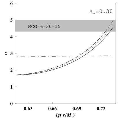
   (a)

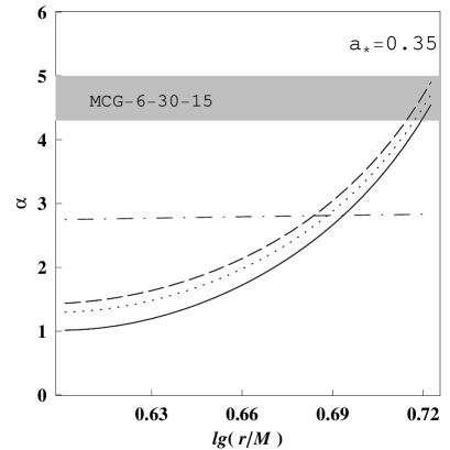
   (b)

Figure 7: The emissivity index of the Seyfert 1 galaxy MCG-6-30-15 inferred from the observation of XMM-Newton is shown in the shaded region. The emissivity index in MCADAF is plotted versus $\lg(r/M)$ for $a_{\ast}$=0.30 and 0.35 in panels (a) and (b), respectively. The curves are plotted for $f$=0.3, 0.325 and 0.35 in solid, dotted and dashed lines, respectively. The emissivity index in ADAF without MC is plotted in dot-dashed line.

Comparing the results in Figure 7 with those obtained in W03, we find that the emissivity index in MCADAF corresponds to the spins less than 0.4, which are much lower than those obtained in MCTHIN with $a_{\ast}>0.99$. By analyzing the X-ray spectrum of the Seyfert 1 galaxy MCG-6-30-15, Dovciak et al. (2004) discussed a low-spin ($a_{\ast}=0.25)$ best-fitting model for the iron line emission in MCG-6-30-15. This result implied that the central BH spin may be low. Brenneman1 and Reynolds (2006) pointed out that an inner emissivity profile requires an inner radius of $r_{inner}=3.2r_{g}$ ($r_{g}\equiv M)$ to fit the iron line emission. These results are consistent with MCADAF but not with MCTHIN, since the inner edge of MCADAF is located at $r_{in}<3.2r_{g}$ for a low BH spin, and the inner emissivity profile can be produced by virtue of the energy transferred in the MC process.

It is shown by the recent observations that the very steep emissivities are also found in XTE J1650-500 (Miller et al. 2002; Miniutti et al. 2004) and GX 339-4 (Miller et al. 2004). The simulations for the steep emissivity in these XRBs can be worked out in the same way as MCG-6-30-15, and the curves of the emissivity index $\alpha$ versus $\lg\left({r\mathord{\left/{\vphantom{rM}}\right.\kern-1.2pt}M}\right)$ for the different values of $a_{\ast}$ and $f$ are shown in Figure 8, from which we find that the BH spins of the two XRBs are also estimated as the low values in fitting the observed very steep emissivity indexes.

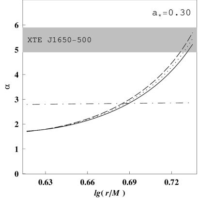
   (a)

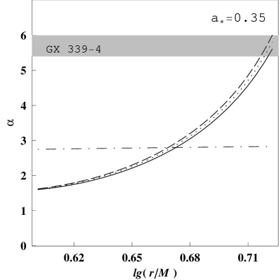
   (b)

Figure 8: The emissivity indexes of XTE J1650-500 (upper panel) and GX 339-4 (lower panel) inferred from the observation of XMM-Newton are shown in the shaded region. The emissivity indexes produced in MCADAF versus $\lg(r/M)$ are plotted in upper panel in solid, dotted and dashed lines for $a_{\ast}$=0.30 with $f$=0.25, 0.275 and 0.3, respectively. Those are plotted in lower panel in solid, dotted and dashed lines for $a_{\ast}$=0.35 with $f$=0.18, 0.2 and 0.22, respectively. The emissivity index produced in ADAF without MC is plotted in dot-dashed line.

4 DISCUSSION

In this paper, we propose a toy model for advection-dominated accretion flows around a rotating BH with the global magnetic field. And the expressions for the extracting power and torque in the MC process and the MC effects on radiation flux are derived. By simulating the emissivity index in Seyfert 1 galaxy MCG-6-30-15 and the two XRBs: XTE J1655-500 and GX 339-4, we find that the steep emissivity index could be interpreted based on MCADAF, and our fittings are consistent with the low BH spins in these sources.

Comparing with MCTHIN and ADAF (or LHAF), the advantage of MCADAF lies in the following aspects.

(1) The electrons of high-temperature in the optically thin plasma are contained in MCADAF, and they are cooled via synchrotron, bremsstrahlung and inverse Compton processes, being responsible for producing hard X-rays spectra in a natural way.

(2) MCADAF providers a natural explanation for transition radius between ADAF and SSD as shown in Figure 1.

(3) MCADAF could be used to interpret the highest luminosity of GX 339-4 in hard-state.

Following W02, we have the energy extracting efficiency in MCADAF as follows:

$$\eta_{{}_{MCADAF}}=\eta_{{}_{ADAF}}+\eta_{{}_{MC}}$$ (32)

where

$$\left\{{\begin{array}[]{l}\eta_{{}_{ADAF}}=1-E_{in},\\ {\eta_{{}_{MC}}=P_{MC}}\mathord{\left/{\vphantom{{\eta_{{}_{MC}}=P_{MC}}\dot{M}}}\right.\kern-1.2pt}\dot{M},\\ E_{in}={\left({1-2\chi_{in}^{-2}+a_{*}\chi_{in}^{-3}}\right)}\mathord{\left/{\vphantom{{\left({1-2\chi_{in}^{-2}+a_{*}\chi_{in}^{-3}}\right)}{\left({1-3\chi_{in}^{-2}+2a_{*}\chi_{in}^{-3}}\right)^{1/2}}}}\right.\kern-1.2pt}{\left({1-3\chi_{in}^{-2}+2a_{*}\chi_{in}^{-3}}\right)^{1/2}}.\end{array}}\right.$$ (33)

By using equations (32) and (33), we have the curves of $\eta_{{}_{MCADAF}}$ and $\eta_{{}_{ADAF}}$ versus $a_{\ast}$, and the ratio of the former to the latter versus $a_{\ast}$ as shown in Figure 9.

   (a)

   (b)

Figure 9: The curves of $\eta_{{}_{ADAF}}$ (solid line) and $\eta_{{}_{MCADAF}}$ (dashed line) versus $a_{*}$ with $f$=0.5; (b) the ratio $\eta_{{}_{MCADAF}}/\eta_{{}_{ADAF}}$ versus $a_{*}$ with $f$=0.5.

From Figure 9, we find that the energy extracting efficiency in MCADAF is greater than that in ADAF for $a_{*}>a_{\ast}^{in}$, and the former could be 1.88 times at most than the latter for $a_{*}=0.9$. This result implies that the luminosity could be augmented significantly in MCADAF. As argued in Y06 the maximum luminosity in LHAF is $L_{LHAF}\approx 16\%L_{E}$, then the maximum luminosity in MCADAF could be $L_{MCADAF}\approx 30\%L_{E}$, which could be used to explain the observation of the highest luminosity of GX 339-4 in hard-state with $25-30\%L_{E}$ (Done & Gierlinski 2003; Zdziarski et al. 2004).

In this paper MCADAF is worked out by combining the MC process with the self-similar solutions given in NY94. However, there exists an obvious inconsistency in this model. The self-similar solution is given based on pesudo-Newtonian potential in NY94, while the MC is formulated in the context of general relativity. Not long ago, some authors (Gammie and Popham 1998; Popham and Gammie 1998) obtained the precise solutions in ADAF in the context of general relativity, and these works provider a possibility to improve MCADAF in our future work.

Acknowledgments. This work is supported by the National Natural Science Foundation of China under Grant Numbers 10573006 and 10121503.

References

• (1)
• (2) Abramowicz M. et al., 1995, ApJ, 438, L37
• (3) Armitage P J and Natarajan P., 1999, ApJ, 523, L7
• (4) Blandford R D 1999 Astrophysical Discs ed Scllwood J A and Goodman J (Astronomical Society of the Pacific Conference Series) 160 265 (astro-ph/9902001)
• (5) Brenneman1 W. L., Reynolds C. S., 2006, accepted by ApJ (astro-ph/ 0608502)
• (6) Done C. & Gierlinski M., 2003, MNRAS, 342, 1041
• (7) Dovciak M. et al., 2004, ApJ Suppl., 153, 205D.
• (8) Esin A. A., McClintock J. E., & Narayan, R., 1997, ApJ, 489, 865
• (9) Gammie C. F. & Popham R., 1998, ApJ, 498, 313
• (10) Lasota J. P. et al., 1996, ApJ, 462, 142
• (11) Lasota J. P., 1998, eds. Abramowicz, Bjornesson, & Pringle, Cambridge Univ. Press, Cambridge
• (12) Li L X. and Paczynski B., 2000, ApJ, 534, L197
• (13) Li L X., 2002a, ApJ, 567, 463 (L02)
• (14) Li L. X., 2002b, A&A, 392, 469
• (15) Macdonald D., Thorne K. S., 1982, MNRAS, 198, 345
• (16) Manmoto T., Mineshige S., Kusunose M., 1997, ApJ, 489, 791
• (17) Miniutti G. et al., 2004, MNRAS, 351, 466
• (18) Miller J. M. et al., 2002, ApJ, 570L, 69M
• (19) Miller J. M. et al., 2004, ApJ, 606, L131
• (20) Narayan R and Yi I., 1994, ApJ, 428, L13 (NY94)
• (21) Narayan R and Yi I., 1995a, ApJ, 444, 231
• (22) Narayan R and Yi I., 1995b, ApJ, 452, 710
• (23) Narayan R., Yi I., Mahadevan R., 1995c, Nature, 374, 623
• (24) Narayan R. et al., 1998, in The Theory of Black Hole Accretion Disks, eds. Abramowicz, Bjornesson, & Pringle, Cambridge Univ. Press, Cambridge.
• (25) Page D. N., Thorne K. S., 1974, ApJ, 191, 499
• (26) Popham R. & Gammie C. F., 1998, ApJ, 504, 419
• (27) Shakura N. I. & Sunyayev R. A., 1973, A&A, 24, 337
• (28) Shapiro S.L., Lightman A.P., & Eardley, D. M., 1976, ApJ, 203, 697
• (29) Wang D. X., Xiao K., and Lei W. H., 2002, MNRAS, 335, 655 (W02)
• (30) Wang D. X., Lei W. H., and Ma R. Y., 2003, MNRAS, 342, 851 (W03)
• (31) Wilms J. et al., 2001, MNRAS, 328, L27
• (32) Yuan F., 1999, ApJ, 521, 55
• (33) Yuan F., 2001, MNRAS, 324, 119 (Y01)
• (34) Yuan F., 2003, ApJ, 594, L99
• (35) Yuan F. et al., 2006, accepted by ApJ (astro-ph/0608552)
• (36) Zdziarski A. A. et al., 2004, MNRAS, 351, 791