Properties of Wide-separation Lensed Quasars by Clusters of Galaxies in the SDSS

Abstract

We use high-resolution $N$-body numerical simulations to study the number of predicted large-separation multiply-imaged systems produced by clusters of galaxies in the SDSS photometric and spectroscopic quasar samples. We incorporate the condensation of baryons at the centre of clusters by (artificially) adding a brightest central galaxy (BCG) as a truncated isothermal sphere. We make predictions in two flat cosmological models: a $\Lambda{\rm CDM}$ model with a matter density $\Omega_{\rm m,0}=0.3$, and $\sigma_{8}=0.9$ ($\Lambda{\rm CDM}$0), and a model favoured by the WMAP three-year data with $\Omega_{\rm m,0}=0.238$, and $\sigma_{8}=0.74$ (WMAP3). We found that the predicted multiply-imaged quasars with separation $>10\arcsec$ is about 6.2 and 2.6 for the SDSS photometric (with an effective area 8000 deg²) and spectroscopic (with an effective area 5000 deg²) quasar samples respectively in the $\Lambda{\rm CDM}$0 model; the predicted numbers of large-separation lensed quasars agree well with the observations. These numbers are reduced by a factor of 7 or more in the WMAP3 model, and are consistent with data at $\la 8\%$ level. The predicted cluster lens redshift peaks around redshift 0.5, and 90% are between 0.2 and 1. The ratio of systems with at least four image systems (${N_{\rm img}}\geq 4$) and those with ${N_{\rm img}}\geq 2$ is about 1/3.5 for both the $\Lambda{\rm CDM}$0 and WMAP3 models, and for both the photometric and spectroscopic quasar samples. We find that the BCG creates a central circular region, comparable to the Einstein ring of the BCG, where the central image disappears in the usual three-image and five-image configurations. If we include four image systems as an extreme case of five-image systems (with an infinitely demagnified central image), we find that 68% of the central images are fainter by a factor of 100 than the brightest image, and about 80% are within $1.5\arcsec$ of the BCG.

1 INTRODUCTION

The number of multiply-imaged quasars lensed by galaxies has now reached roughly one hundred. The typical separation of these systems ranges from $0.3-6\arcsec$. They provide an valuable sample to constrain the cosmological constant, the Hubble constant, and the mass profiles of lensing galaxies at intermediate redshift (for an extensive review, see Kochanek, Schneider & Wambsganss 2006 and references therein).

The search for multiply-imaged quasars by clusters of galaxies has been less successful. The initial search for wide-separation radio sources yielded no successful candidates between $6-15\arcsec$ (Phillips et al. 2001a), and from $15-60\arcsec$ (Phillips et al. 2001b). Ofek et al. (2001) also failed to find any wide-separation quasars between $5-30\arcsec$ in the FIRST 20-cm radio survey. The lack of cluster lensed radio sources is likely due to the small number of radio sources surveyed ($\sim$ 20,000). The breakthrough came from the Sloan Digital Sky Survey (SDSS) where a large number of optical quasars became available. So far, there are approximately 46,420 spectroscopically confirmed broad-line quasars in SDSS Date Release 3. Two spectacular cluster lenses were discovered in the SDSS (not limited to DR3, see §4.2). The first case was SDSS J1004+4112, a quadruply-imaged system with an separation of 14.6 arcsec (Inada et al. 2003; Oguri et al. 2004). The cluster is at redshift of 0.68, and the lensed quasar is at redshift 1.734. A faint fifth image was later discovered (Inada et al. 2005), as were many other multiply-imaged background galaxies (Sharon et al. 2005). The second case, SDSS J1029+2623, was a double-image system with a separation of 22.5 arcsec. The lensing cluster is likely at redshift 0.55 (Inada et al. 2006), and the background quasar at redshift $z_{\rm s}=2.197$.

Cluster lenses, just like galaxy-scale lenses, provide valuable constraints on the lens mass profiles. They are also important because the number of such lenses depend quite sensitively on the cosmology, in particular the matter power-spectrum normalisation, $\sigma_{8}$, and the matter density, $\Omega_{\rm m,0}$. This sensitivity has already been explored using giant arc statistics where the lensed sources are background galaxies, rather than quasars (e.g., Meneghetti et al. 2003a, b; Wambsganss et al. 2004; Torri et al. 2004; Dalal et al. 2004; Horesh et al. 2005; Li et al. 2005; Oguri et al. 2003). The analysis by Li et al. (2006b) prefers a high $\sigma_{8}$ universe. However, the study and other similar ones suffer from one deficiency, namely the properties of the lensed background galaxy population, in particular their redshift distribution, is not well known, so the conclusion is somewhat uncertain.

In comparison, the quasar population has a much better-known redshift distribution, and so does not suffer as much from the same deficiency, hence a careful analysis of the statistics of multiply-imaged quasars is complementary to those of giant arcs. Of course, the number of known multiply-imaged quasars so far is very small (two), compared to hundreds of known giant arcs (e.g., Luppino et al. 1999; Gladders et al. 2003; Zaritsky & Gonzalez 2003; Sand et al. 2005; Hennawi et al. 2006). Nevertheless, even this small sample provides interesting constraints. For example, the analysis of Oguri et al. (2004) of the first cluster lens, J1004+4112, concluded that the $\sigma_{8}$ value must be high, $\sigma_{8}=1^{+0.4}_{-0.2}$ (95% confidence) even for an inner density profile, $\rho\propto r^{-1.5}$, considerably steeper than the NFW profile ($\rho\propto r^{-1}$ for small $r$, Navarro, Frenk & White 1997). Many studies of clusters of galaxies prefer the NFW profile (e.g., van de Marel et al. 2000; Comerford et al. 2006; Voigt & Fabian 2006). For such a shallower profile, the required $\sigma_{8}$ would be even higher.

Another advantage of lensed quasars concerns the lens selection. For giant arc surveys, observers first select clusters from optical or X-ray data and then take deep followup images, hence the discovery of giant arcs depends on how clusters are selected in the first place. On the other hand, lensed quasars are usually identified by examining quasars to see whether they are multiply imaged. In other words, current arc surveys only observe biased directions whereas quasar lenses survey random line-of-sight. In addition, quasars are point sources, so one does not have complications arising from seeings, background source size and ellipticity distributions etc, thus it is much simpler to model the quasar source population.

There have been many previous works to predict the abundance of large-separation quasar lensed by massive dark halos using simple spherical models (Maoz et al. 1997; Sarbu et al. 2001; Keeton & Madau 2001; Wyithe et al. 2001; Li & Ostriker 2002; Rusin 2002; Li & Ostriker 2003; Oguri 2003; Huterer & Ma 2004; Lopes & Miller 2004; 2004; Oguri et al. 2004; Chen 2004). In particular, Lopes & Miller (2004), using spherical clusters, found that wide-separation lensed quasars can be a powerful tool to measure $\sigma_{8}$ and $\Omega_{m,0}$. Using triaxial halo models, Oguri & Keeton (2004) computed the abundance of quasars multiply imaged by clusters analytically and found that triaxiality significantly increases the expected number of lenses. Hennawi et al. (2007b) presented the first predictions of multiply-imaged quasars using N-body simulated clusters in the a flat cosmology with $\Omega_{\rm m,0}=0.3$, $\Omega_{\Lambda,0}=0.7$ with $\sigma_{8}=0.95$. In this paper, we compare the predictions for the cosmology favoured by the three-year WMAP result with the usual concordance cosmology. We also make more detailed predictions for cluster lenses as a function of image multiplicity, and study the brightness of the central images and their offset from cluster centres.

The paper is structured as follows. In §2, we discuss the simulations we use and our lensing methodology. In §3, we discuss the background source population, namely the quasar luminosity function. In §4, we present the main results of the paper, and we finish in §5 with a summary and a discussion of the implications of our results.

2 NUMERICAL SIMULATIONS AND LENSING METHODOLOGY

In this paper, we utilise two sets of simulations, one for the ‘standard’ $\Lambda{\rm CDM}$ model with $\sigma_{8}=0.9$, and the other for the cosmological model given by the recent three-year WMAP data with $\sigma_{8}=0.74$ (Spergel et al. 2006). For brevity, these two models will be referred to as $\Lambda{\rm CDM}$0, and WMAP3, respectively, and the corresponding cosmological parameters are:

1. $\Lambda{\rm CDM}$0:  $\Omega_{\rm m,0}=0.3,\Omega_{\Lambda,0}=0.7,h=0.7,\sigma_{8}=0.9,n=1$;

2. WMAP3: $\Omega_{\rm m,0}=0.238,\Omega_{\Lambda,0}=0.762,h=0.73,\sigma_{8}=0.74,n=0.95$,

where $h$ is the Hubble constant in units of $100\,\rm km\,{s}^{-1}\,\rm Mpc^{-1}$, and $n$ is the spectral index of the power spectrum. The assumed initial transfer function in each model was generated with CMBFAST (Seljak & Zaldarriaga 1996). Notice that both $\sigma_{8}$ and $\Omega_{\rm m,0}$ differ in these two models, and both will impact on the number of multiply-imaged quasars.

Table 1: Parameters for the two cosmological numerical simulations. The columns are cosmology, box size, number and mass of dark matter particles, and the softening length.

model	box size	$N_{\rm DM}$	$m_{\rm DM}$	softening
	$(h^{-1}\,\rm Mpc)$		$(h^{-1}M_{\odot})$	($h^{-1}$ kpc)
$\Lambda{\rm CDM}$0	300	$512^{3}$	$1.67\times 10^{10}$	30
WMAP3	300	$512^{3}$	$1.32\times 10^{10}$	30

We use a vectorised-parallel ${\rm P^{3}M}$ code (Jing & Suto 2002) and a PM-TREE code – GADGET2 (Springel, Yoshida, & White, 2001; Springel, 2005) to simulate the structure formation in these models; the details of the simulations are given in Table 1. Both are $N$-body simulations which evolve $N_{\rm DM}=512^{3}$ dark matter particles in a large cubic box with sidelength equal to $300h^{-1}\,\rm Mpc$. The $\Lambda{\rm CDM}$0 simulation was performed using the ${\rm P^{3}M}$ code of Jing & Suto (2002) and has been used in Li et al. (2005) to study the properties of giant arcs. We refer the readers to that paper for more details. The WMAP3 simulation was carried out with GADGET2, and has been used by Li et al. (2006b) to compare the statistics of giant arcs in the $\Lambda{\rm CDM}$0 and WMAP3 models. Similarly, in this work we will use them to compare the statistics of multiply-imaged quasars in these two cosmological models. We return to the issue of cosmic variance in §4.4.

Dark matter halos are identified with the friends-of-friends method using a linking length equal to 0.2 times the mean particle separation. The halo mass $M$ is defined as the virial mass enclosed within the virial radius according to the spherical collapse model (Kitayama & Suto 1996; Bryan & Norman 1998; Jing & Suto 2002).

For any given cluster, we calculate the smoothed surface density maps using the method of Li et al. (2006a). Specifically, for any line of sight, we obtain the surface density on a $1024\times 1024$ grid covering a square of (comoving) side length of $4h^{-1}\,\rm Mpc$ centreed on each cluster. The projection depth is also chosen to be $4h^{-1}\,\rm Mpc$. Notice that the size of the region is large enough to include all particles within the virial radius (in fact, several virial radii for small clusters). Particles outside this cube and large-scale structures do not contribute significantly to the lensing cross-section (e.g. Li et al. 2005; Hennawi et al. 2007a), so we will ignore their contributions here.

Our projection and smoothing method uses a smoothed particle hydrodynamics (SPH) kernel to distribute the particle mass on a three-dimension grid and then the surface density is obtained by integrating along the line of sight (see Li et al. 2006a for more detail). In this work, the number of neighbours used in the SPH smoothing kernel is fixed to be 32. We calculate the surface density along three orthogonal directions for each cluster. Once we obtain the surface density of a dark matter halo, its lensing potential, $\phi_{\rm DM}$, can then be easily calculated using the Fast Fourier Transform (FFT).

Many clusters of galaxies have a very luminous central galaxy. The effect of such brightest cluster galaxies (BCGs) has been quantified by Hennawi et al. (2007b). For multiply-imaged systems with separations $\lesssim 20\arcsec$, BCGs can enhance the cross-section by $\sim$ 50%. Following Hennawi et al. (2007b), we also artficially add a BCG at the centre of each cluster. This is obviously a simplification as BCGs are assembled as a function of time; we briefly return to this issue in the discussion. The BCG is modelled as a truncated isothermal sphere. The mass of BCG is taken to be a fixed fraction of the host halo, $M_{\rm BCG}=3\times 10^{-3}M_{\rm FOF}$ and its velocity dispersion is given by

$$\frac{\sigma}{300\,\rm km\,{s}^{-1}}=\left(\frac{M_{\rm FOF}}{10^{15}\rm M_{\odot}}\right)^{2/15}.$$ (1)

The truncation radius is given by $r_{\rm max}=GM_{\rm BCG}/(2\sigma^{2})$. See Hennawi et al. (2007b) for more details.

In the following we will only present results including such a BCG, which approximately accounts for the effects of baryonic cooling at the centre of clusters. The effect of baryons in non-central galaxies is likely to be smaller. As the BCG is modelled as a truncated isothermal sphere, its lensing potential, $\phi_{\rm BCG}$, can be calculated analytically. The total lensing potential is a sum of the contributions from the (pure) dark matter halo and the BCG, $\phi=\phi_{\rm DM}+\phi_{\rm BCG}$. The deflection angle ($\vec{\alpha}$) and magnification ($\mu$) can be obtained by taking first-order and second-order derivatives with respect to $x$ and $y$, $\alpha_{x}=\phi_{x}$, $\alpha_{y}=\phi_{y}$, and $\mu=[(1-\phi_{xx})(1-\phi_{yy})-\phi_{xy}^{2}]^{-1}$. We calculate the BCG contribution to the deflection angle and potential analytically, and the dark matter halo contribution using FFT as discussed above.

Using these derivatives, we can create the mapping from the image plane to the source plane and obtain the critical curves and caustics. Critical curves are a set of image positions with $\mu=\infty$, and the caustics are the corresponding source positions. Caustics play a crucial role in gravitational lensing as they divide the source plane into regions of different image multiplicities. Whenever a source crosses a caustic, the image number either increases or decreases by two. For a quasar to be multiply-imaged, it must lie inside one of the caustics.

To calculate the cross-section of a given separation of a multiply imaged quasar, we first find the smallest rectangle which encloses all the caustics, and then a regular grid is created dividing this rectangle into pixels of $0.3\arcsec$ by $0.3\arcsec$. For each source position located on the grid, we find the corresponding image positions and magnifications ($\mu$) using the Newton-Raphson method. For a given multiple-image system, the number of images one can observe, ${N_{\rm img}}$, depends on the magnification of each image, the source intrinsic magnitude and the survey magnitude limit. For such systems, we sort the images according to the image magnifications and record the number of images ${N_{\rm img}}$ and the maximum separation $\Delta\theta$ between these ${N_{\rm img}}$ images. We then examine whether the multiple images satisfy the observational selection criteria (see §3.1). For given lens and source redshifts, $z_{\rm l}$ and $z_{\rm s}$, collecting systems that pass the selection allows us to construct a cross-section $\sigma(\geq{N_{\rm img}},>\theta|z_{\rm l},z_{\rm s})$ for lensing systems with at least ${N_{\rm img}}$ images and separations larger than $\theta$.

The SDSS photometric and spectroscopic quasar samples are magnitude limited, multiply-imaged quasars will be over-represented in such samples due to the lensing magnification (Turner 1980). To account for this magnification (or amplification) bias, we further divide the cross-section into 50 bins of $\Delta m\equiv-2.5\log\mu$ from $-5$ mag to 5 mag with a bin size of 0.2 mag, and obtain a differential cross-section $d\sigma/d\Delta m(\geq{N_{\rm img}},>\theta|{\Delta m},z_{\rm l},z_{\rm s})$.

As in Li et al. (2005), we can obtain the total cross-section per unit comoving volume by summing over the contributions of all the clusters:

$$\overline{\sigma}(\geq{N_{\rm img}},>\theta|\Delta m,z_{\rm l},z_{\rm s})={\sum\sigma_{i}(\geq{N_{\rm img}},>\theta|\Delta m,z_{\rm l},z_{\rm s})\over V},$$ (2)

where $\sigma_{i}(\geq{N_{\rm img}},>\theta|\Delta m,z_{\rm l},z_{\rm s})$ is the average cross-section of the three projections of the $i$-th cluster at redshift $z_{\rm l}$, $z_{\rm s}$ is the source redshift, and $V$ is the comoving volume of the simulation box. Then, accounting for the magnification bias (for more detailed descriptions, see Sect. 3.1), the predicted number of large-separation lens can be derived as:

$$N(\geq{N_{\rm img}},>\theta)= \int_{0}^{\infty}dz_{\rm s}\int_{0}^{z_{\rm s}}dz_{\rm l}\int_{-\infty}^{+\infty}d\Delta m\,\,$$

$${d{\overline{\sigma}}\over d{\Delta m}}(\geq{N_{\rm img}},>\theta|{\Delta m},z_{\rm l},z_{\rm s})$$

$$\times n(<i_{0}-{\Delta m},z_{\rm s})\,(1+z_{\rm l})^{3}\,\,{dV_{\rm p}(z_{\rm l})\over dz_{\rm l}}$$ (3)

where $n(<i,z_{\rm s})\times dz_{\rm s}$ is the number of quasars brighter than the SDSS $i$-band magnitude $i$ in the redshift interval from $z_{\rm s}$ to $z_{\rm s}+dz_{\rm s}$, $i_{0}$ is the flux limit, and $dV_{\rm p}(z_{\rm l})$ is the proper volume of a spherical shell with redshift from $z_{\rm l}$ to $z_{\rm l}+dz_{\rm l}$. We used 22 simulation output with redshift from 0.1 to 2, and selected the 600 (for $\Lambda{\rm CDM}$0) or 400 (for WMAP3) most massive clusters in each output to calculate the total lensing cross-sections. The lowest masses of clusters in these two cosmologies are $7.8\times 10^{13}h^{-1}M_{\odot}$ and $5\times 10^{13}h^{-1}M_{\odot}$ respectively at redshift 0.5. The integration step size of $z_{\rm l}$ is the same as the redshift interval of simulation output ($\delta z_{\rm l}\approx 0.1$) and the source redshift is at 0.7, 1.0, 1.5, 2.0, 2.5, 3.0, 3.5, 4.0, 4.5, 5.0 and 5.5.

3 THE QUASAR LUMINOSITY FUNCTION

To make accurate predictions for the frequency of multiply-imaged quasars, we must specify the quasar luminosity function as a function of redshift and luminosity. Following Boyle et al. (2000), we will use a double power-law to parameterise the quasar luminosity function

$$\Phi(M,z)=\frac{\Phi^{\ast}(z)}{10^{0.4(\beta_{l}+1)[M-M^{\ast}(z)]}+10^{0.4(\beta_{h}+1)[M-M^{\ast}(z)]}},$$ (4)

where $M$ is the absolute magnitude in a filter, and $\Phi^{\ast}$ and $M^{\ast}$ are the characteristic density and magnitudes respectively in a certain band.

For the low redshift ($z<2.1$) quasars, we use the parameters from the 2dF-SDSS LRG and QSO (2SLAQ) Survey (Richards et al. 2005). The luminosity function is fitted in the SDSS $g$-band with $\beta_{l}=-1.45$, $\beta_{h}=-3.31$ and $\Phi^{\ast}=1.83\times 10^{-6}\rm\,Mpc^{-3}\,mag^{-1}$. The characteristic luminosity in the $g$-band, $M^{\ast}_{g}$, is described by a second-order polynomial of redshift:

$$M^{\ast}_{g}(z)=M^{\ast}_{g}(0)-2.5(k_{1}z+k_{2}z^{2}),$$ (5)

where $M^{\ast}_{g}(0)=-21.61$, $k_{1}=1.39$ and $k_{2}=-0.29$.

For high redshift, $z>3.5$, quasars, we take the parameters from Fontanot et al (2006), which were obtained from a joint analysis of the GOODS and SDSS data. The best fit to the luminosity function as a function of the monochromatic 1450 Å  magnitude, $M_{145}$, gives $\beta_{l}=-1.71$, $\beta_{h}=-3.31$; the data also prefers a pure density evolution with an exponential form:

$$\Phi^{\ast}(z)=\Phi^{\ast}_{(z=2)}e^{k_{z}[(1+z)-3]},$$ (6)

where $k_{z}=-1.37$ and $\Phi^{\ast}_{(z=2)}=1.67\times 10^{-6}\rm\,Mpc^{-3}\,mag^{-1}$. The characteristic monochromatic luminosity, $M^{\ast}_{145}$, is fixed at $\rm M^{\ast}_{145}=-26.43$.

For a given flux limit $i_{0}$, we can easily obtain the total number density of quasars $\rm n(<i_{0},z)$ in the redshift space for $z<2.1$ and $z>3.5$. However, the quasar luminosity function is not well constrained from redshift 2.1 to redshift 3.5. For a given magnitude limit $i_{0}$, we estimate the number density of quasar with redshift $2.1<z<3.5$ by linear interpolation as a function of redshift of the quasar number densities with the same absolute magnitude. For a given redshift $z$, we first calculate the corresponding absolute magnitude, $M^{0}_{i}(z)$ for each apparent magnitude $i$. We then convert this, using k-corrections (see §3.1), into corresponding $g$-band and the 1450 Å  monochromatic absolute luminosities at $M^{0}_{g}$ and $M^{0}_{145}$ at redshift $z$. Since we know $\Phi(M^{0}_{g},z=2.1)$, $\Phi(M^{0}_{145},z=3.5)$, we obtain the $\Phi(M_{i},z)$ by linear interpolation:

$$\Phi(M_{i},z)=\frac{\Phi(M^{0}_{g},2.1)\times(3.5-z)+\Phi(M^{0}_{145},3.5)\times(z-2.1)}{3.5-2.1}.$$ (7)

We can then simply integrate the above equation to derive the number density of quasars per square degree for any limiting magnitude $i$.

We also consider the incompleteness of quasars at redshift from 2.3 to 3.6 as in Hennawi et al. (2007b). The SDSS spectroscopic and photometric surveys depend on colour selection and the colours of quasars and stars are not easy to disentangle in this redshift range. So we assume that only 60% of quasars in this redshift interval are found by the SDSS.

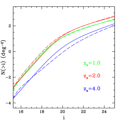
Figure 1: The left panel shows the redshift distribution of quasars for a flux limit of $i<22.7$. Three redshift intervals ($z_{\rm s}\sim 1,2$ and 4) are indicated by the vertical lines. The shaded region corresponds to the 60% completeness we assumed. The right panel shows the surface density of quasars as a function of the SDSS $i$-band magnitude for the three source redshift intervals. The solid and dashed lines show the shapes used by us and by Hennawi et al. (2007b) respectively. They are in good agreement for the two low redshift intervals, but for high reshift interval, our amplitude is higher by roughly a factor of 2 than theirs between $i=18$ and 22.

3.1 The cross filter k-correction, quasar samples and lens selection

The SDSS spectroscopic and photometric survey have flux limits in the $i$-band but the parameters in the above luminosity functions (in eqs. 4-7) are given in different bands, $M_{g}$ and $\rm M_{145}$. To apply these quasar luminosity functions to the $i$-band, we have to do cross filter k-corrections (Hogg et al. 2002). We use the results of Richards et al. (2006) who provided the k-correction from the SDSS i-band to the SDSS $g$-band and the monochromatic 1450 Å  absolute magnitude assuming a power-law quasar spectral index, $\alpha_{\nu}=-0.5$.

As in Hennawi et al. (2007b), we use the same photometric and spectroscopic quasar samples. For the SDSS spectroscopic quasar sample, the covered area is about 5000 $\rm deg^{2}$ and the magnitude limit is $i<19.1$ for low redshift ($z<2.5$) quasars and $i<20.2$ for high redshift ($z>2.5$) quasars (Schneider et al. 2005). The faint SDSS photometric quasar survey covers a larger area, $\sim 8000\,\rm{deg}^{2}$, with a flux limit of $i<21.0$ for $z<2.5$ and $i<20.5$ for $z>2.5$ (Richards et al. 2004). To select lenses in the photometric and spectroscopic quasar samples, we require the brightest image to be brighter than the magnitude limit given above, and other images to be brighter than $i=21.0$, after accounting for their magnifications. The fainter limit for other images is because of fiber collisions in the SDSS, usually only one quasar image will be spectroscopically targeted, while other quasar candidates have to be confirmed with other, typically larger telescopes that can reach much fainter magnitudes. This is what actually occurred for the discovery of the first two lenses, and so we will adopt this selection criterion, similar to Hennawi et al. (2007b). Notice that some images may still be missed if they are below the flux limit, even after the magnification, so the observed number of images may be smaller than the intrinsic number.

Notice that the photometric sample goes almost two magnitudes deeper than the spectroscopic sample for quasars below redshift 2.5 (magnitude limit 21.0 vs. 19.1), but only slightly deeper for high redshift quasars (20.2 vs. 20.5). As a result, the photometric sample has many more low-redshift quasars compared with the spectroscopic sample. This will be reflected in the source and lens redshift distributions for multiply-imaged quasars (see Figs. 6 and 7).

Fig. 1 shows the redshift distribution of quasars for $i<22.7$. It shows the well known peak around redshift 2, and the sharp decline beyond redshift 4. The shaded region corresponds to the 60% completeness we assumed. This result is in good agreement with the left panel of Fig. 1 in Hennawi et al. (2007b). Notice that the geometries in the $\Lambda{\rm CDM}$0 and WMAP3 cosmologies are different, due to the small difference in the matter density. However, even for a source at redshift 5, the angular diameter distance differs only by $<8\%$. Furthermore, we reproduce the quasars distribution as a function of redshift and magnitude (see Fig. 1) using our luminoisty functions. This distribution is directly comparable with the observations and model independent. Our calculation in each cosmology is based on this quasar distribution. So the small cosmological dependence of the luminosity function is accounted for. The left panel also indicates three redshift intervals ($z\sim 1,2$ and 4), for which we show the surface density of quasars as a function of magnitude limit. The dashed lines show the corresponding results of Hennawi et al. (2007b). Our results are consistent with theirs for the two low redshift intervals, but for the highest redshift interval ($z\sim 4$), our quasar surface density is roughly a factor of two of that of Hennawi et al. (2007b) between $i=18$ and 22. As we use the updated results by Richards et al. (2005), our luminosity function may be more realistic than that in Hennawi et al. (2007b). It is worth emphasising, however, that this difference has only moderate effects on the number of predicted multiply-imaged quasars because most ($\sim 75\%$ and $\sim 70\%$) of the lensed sources are below redshift 3 for the photometric and spectroscopic samples.

4 RESULTS

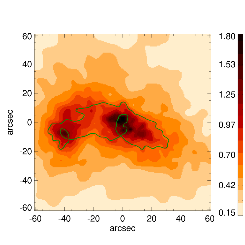
Figure 2: The surface density map (in units of the critical surface density) for the most massive cluster at redshift $z_{\rm l}=0.5$ in the $\Lambda{\rm CDM}$0 simulation (in one projection). The cluster virial mass is $1\times 10^{15}h^{-1}M_{\odot}$. The colour bar at the right shows the scales. Notice that the main cluster (located at the origin) is merging with a sub-cluster at the left. The critical curves (appropriate for a source at redshift 2.5) are shown as the green curves (see also Fig. 3.)

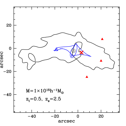
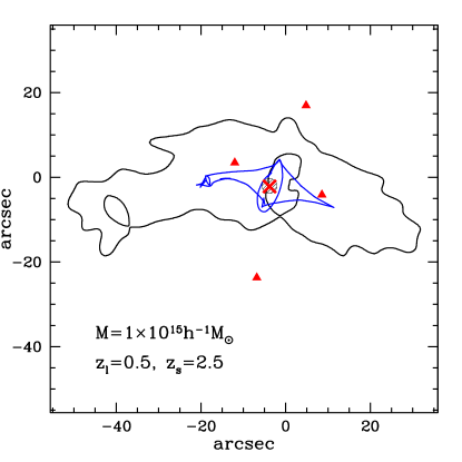
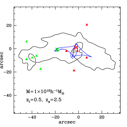
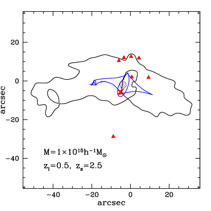
Figure 3: Example image configurations for the most massive cluster at $z_{\rm l}=0.5$ in our $\Lambda{\rm CDM}$0 simulation shown in Fig. 2. The source is assumed to be at redshift $z_{\rm s}=2.5$. The cluster mass is $1\times 10^{15}h^{-1}M_{\odot}$. The blue and black curves are the caustics and critical curves respectively. For each panel, the red cross shows the source position and the corresponding images are shown as triangles. The bottom left panel shows an additional source position (green cross) and the corresponding images are shown as green triangles. When a source lies in the shaded circle, the central image disappears. This is a result of approximating the Brightest Cluster Galaxy (BCG) as a truncated isothermal sphere (see the discussion in §4.1).

Armed with knowledge of the background source population and cluster lensing cross-sections, we can now make detailed predictions for multiply-imaged quasars in the SDSS. We start with an example cluster and illustrate possible multiply-imaged configurations in §4.1. We then discuss statistical properties of multiply-imaged quasars, including the total number and partitions in different image multiplicities, for both the $\Lambda{\rm CDM}$0 and WMAP3 cosmologies in §4.2. In §4.3 we examine the properties of central images, and finish with a discussion of cosmic variance in §4.4.

4.1 An example cluster: caustics, critical curves and images

Fig. 2 shows the projected surface density map (along one direction) for the most massive cluster in the $\Lambda{\rm CDM}$0 cosmology at redshift 0.5. This cluster has a mass of about $10^{15}h^{-1}M_{\odot}$. It can be seen that in addition to the massive cluster located close to the origin, there is another sub-cluster located roughly $40\arcsec$ away (corresponding to $170h^{-1}\,\rm kpc$ away in projection) to the left merging with the main cluster shown at the origin.

The critical curves and caustics for this cluster are shown in Fig. 3. Both are quite elongated along the horizontal axis, partly due to the shear of the merging sub-cluster. Notice that there is also a small, inner critical curve associated with the sub-cluster. The caustics consist of an inner ellipse and an outer diamond (there are small intersections, however). There are also high-order singularities such as swallowtails in the caustics. Sources located inside such high-order singularity regions can produce image numbers higher than 5 (see the bottom right panel).

The top left panel of Fig. 3 shows an image configuration where the source is located just inside the outer diamond caustic. All three formed images are quite far away from the centre of the main cluster. When the source moves into the inner ellipse, we normally expect five images. However, as a consequence of modelling the BCG as a truncated singular isothermal sphere, we find that there is a roughly circular region (shaded in the Figure) within which the central, fifth image disappears – the central image has been ‘swallowed’ by the BCG. The radius of this region is roughly one angular Einstein radius corresponding to the isothermal sphere, $4\pi(\sigma/c)^{2}D_{\rm ls}/D_{\rm s}$, where $D_{\rm ls}$ is the angular diameter distance between the lens and source, and $\sigma$ is the velocity dispersion (cf. eq. 1). Such a four-image configuration is illustrated in the top right panel. We can regard such cases as an extreme example of a five-image configuration where the central image has been infinitely de-magnified.

The bottom left panel in Fig. 3 shows a source position that produces the usual five-image systems. As expected, the fifth image is close to the cluster centre. There is, however, a different kind of five image configuration, which is produced by the presence of the sub-cluster. As we only put in (by hand) a BCG at the centre of the main cluster, the central image induced by such sub-clusters is always present, and will be located close to the centre of the sub-cluster, and in general much further away from the main cluster centre (see also Fig. 9).

For rare cases, when the source is located in regions of high-order singularity, the image number can exceed 5. One example is shown in the bottom right panel. For this case, four images are clustered close together, tangentially aligned with a critical curve, while the other three images are further apart. It can be seen from Fig. 3 that such high-order singularity regions are rare, and so we do not expect a significant fraction of sources to have image numbers exceeding five.

For other clusters in our simulations, the image configurations are similar except that for some small clusters, we can also have two-image configurations. These are the usual three-image systems for which the central image has been ‘swallowed’ by the BCG, similar to the four-image case discussed above.

4.2 Expected number of multiply-imaged quasars in the SDSS

Figure 4: The top panel shows the number of predicted large-separation multiply-imaged quasars as function of separation for the $\Lambda{\rm CDM}$0 (top two curves) and WMAP3 (bottom curves) models, while the solid and dashed lines are for the SDSS photometric (with an effective area of $\sim$ 8000 deg²) and spectroscopic (with an effective area of $\sim$ 5000 deg²) quasars sample respectively. The bottom panel shows the ratio of the predicted numbers in the two cosmologies. Notice that the ratio increases as the separation increases.

The expected number of multiply-imaged quasars in the SDSS is shown in Fig. 4 for the photometric (solid) and spectroscopic (dashed) samples, in both the $\Lambda{\rm CDM}$0 (top two curves) and WMAP3 (bottom curves) cosmologies. In the $\Lambda{\rm CDM}$0 cosmology, we expect 6.2 and 2.6 lenses with separations larger than $10\arcsec$ for the photometric (with an effective area of $\sim$ 8000 deg²) and spectroscopic (with an effective area of $\sim$ 5000 deg²) samples respectively. The corresponding numbers are much lower in the WMAP3 model, about 0.85 and 0.36 respectively. The bottom panel of Fig. 4 shows the relative ratios in these two cosmologies – the ratio is about $\sim 7$ at $10\arcsec$, but increases to about $\sim 11$ at $30\arcsec$, for both samples.

The large reduction factor in the WMAP3 model is a direct result of the lower abundance of clusters in this cosmology compared with $\Lambda{\rm CDM}$0 (see Fig. 10) because of the lower $\sigma_{8}$ and lower mass density $\Omega_{\rm m,0}$. The reduction factor is larger for more massive clusters. This explains the separation dependence of the ratio because larger separation lenses are produced by more massive clusters. The reduction factor is comparable to that of giant arcs ($\sim 6$) for $\theta>10\arcsec$ but larger by a factor of 2 for $\theta>30\arcsec$. The substantially lower number of predicted multiply-images in the WMAP3 model may be somewhat difficult to reconcile with the data; we will return to this point at the end of this section.

Figure 5: The number of large-separation multiply-imaged quasars as function of separation and image multiplicity for the SDSS photometric (with an effective area of $\sim$ 8000 deg²) and spectroscopic (with an effective area of $\sim$ 5000 deg²) quasar samples. The top and bottom panels show the results for the $\Lambda{\rm CDM}$0 and WMAP3 cosmologies respectively. For each panel, from top to bottom, the lines are for ${N_{\rm img}}\geq 2,3,4,5$ respectively. The two crosses show the predicted positions of the two known large-separation lenses.

We can further divide the predicted number of multiply-imaged quasars by clusters according to the image multiplicity. The results are shown in Fig. 5 for the two quasar samples in the $\Lambda{\rm CDM}$0 and WMAP3 cosmologies. While the amplitudes differ, the relative ratios of lenses with ${N_{\rm img}}\geq$ 2, 3, 4, and 5 are quite similar. For example, the number of systems with ${N_{\rm img}}\geq 4$ is about 1/3.5 of the number of systems with ${N_{\rm img}}\geq 2$.

It is interesting to ask for multiply-imaged quasars, what are the typical redshifts of lensing clusters and background quasars. These are important for observationally identifying the lensing candidates. Fig. 6 shows the differential number distribution for the lens redshift. The distributions are similar in the $\Lambda{\rm CDM}$0 and WMAP3 cosmologies; both peak around redshift 0.5, and 90% of the lensing clusters are predicted to be between redshift 0.2 and 1. The predicted lens redshift distribution is in good agreement with Hennawi et al. (2007b). Notice that the median redshift for the lenses in the spectroscopic sample is slightly higher than that for the photometric sample. This can be understood as follows: quasars in the spectroscopic sample are on average at higher redshift, since the most likely lens location is roughly mid-way between the lens and source, as a result the lens redshift is also slightly higher. The two observed cluster lenses have redshifts 0.55 and 0.68, roughly at the position of the peak, in good agreement with the theoretical expectations.

The corresponding source redshift distribution is shown in Fig. 7. The distributions are again similar in the two cosmologies. For the multiply-imaged quasars in the photometric sample, their redshift distribution peaks around redshift 2, while for the spectroscopic quasar sample, the peak is extended with a range from 2 to 3. This is again a result of the lower source redshift in the photometric sample (see §3). The two observed source redshifts (1.734 for J1004+4112, and 2.197 for J1029+2623) coincides with the peak predicted for the photometric sample, but appears to be at the low side for the the spectroscopic sample (but unlikely to be statistically significant due to the limited number statistics).

Figure 6: The lens redshift distribution in the $\Lambda{\rm CDM}$0 cosmology (left) and WMAP3 cosmology (right). The area under each curve is normalised to the total number of multiply-imaged quasars. The two vertical bars show the lens redshifts of SDSS J1004+4112 (0.68) and SDSS J1029+2623 (0.55). The shapes are similar in these two cosmologies. Notice that the median lens redshift is slightly lower for the photometric quasar sample (see §3).

Figure 7: The source redshift distribution of multiply-imaged quasars with separation $>10\arcsec$ in the $\Lambda{\rm CDM}$0 (left) and WMAP3 (right) models. The peak of the source redshift distribution shifts to lower redshift in the photometric sample due to the lower mean quasar redshift for this sample (see §3). The vertical bars show the sources redshifts for SDSS J1004+4112 (1.734) and SDSS J1029+2623 (2.197).

It is interesting to explore whether these two cosmologies are consistent with the data, given even the very limited number of cluster lenses. The effective area for the Data Release 5 of the SDSS is 5740 deg². J1029+2623 is from SDSS-II, which has now discovered about 10,000 QSOs, which is roughly 1/4 of the QSOs discovered in the Data Release 3, which has an area of about 3700 deg², so these two lenses were discovered in an effective area of $\sim 5740+3700/4\approx 6500$ deg² in the SDSS spectroscopic sample. In the $\Lambda{\rm CDM}$0 model, the two crosses in the top left panel in Fig. 5 shows the positions we predict, (14.6, 0.55) and (22.5, 0.93) for these two systems. The number of lenses with separation larger than $14.6\arcsec$ quadrupole-images (J1004+4112) and $22.5\arcsec$ double images (J1029+2623) are $0.55\times 6500/5000=0.7$ and $0.93\times 6500/5000=1.2$. This is roughly consistent with what we have discovered in the SDSS so far. However, for the WMAP3 model, the positions of crosses in the bottom left panel in Fig. 5 are (14.6 0.072) and (22.5 0.094). The number of lenses with separation larger than $14.6\arcsec$ quadrupole-images and $22.5\arcsec$ double images are $0.072\times 6500/5000=0.094$ and $0.11\times 6500/5000=0.14$ for the SDSS spectroscopic sample with an effective area of $\sim$6500 deg². We conservatively estimate the probability of observing such two systems in WMAP3 model as follows. The predicted number of lensed quasar systems with ${N_{\rm img}}\geq 2$ and $\theta>10\arcsec$ is 0.36$\times$6500/5000= 0.468. Assuming a Poisson distribution with a mean number of lenses $\lambda=0.468$, the probability of observing these two systems in WMAP3 model is, $P(N\geq 2)=1-P(0)-P(1)=1-e^{-\lambda}-\lambda e^{-\lambda}\sim 8\%$. So even with the very limited sample of two multiply-imaged quasars, it seems that the WMAP3 cosmology is compatible with observations only at $\sim 8\%$ level. Considering that our lensing optical depth may be over-estimated in the WMAP3 model due to cosmic variance (see §4.4), and the fact that the number of observed systems may be a lower limit (due to possible incompleteness in the surveys), so the probability may be even lower ($\lesssim 4\%$) in reality.

4.3 Properties of central images

For non-singular lensing potentials, catastrophe theory predicts generically an odd number of images (Burke 1981). However, for nearly all galaxy-scale lenses (with the exception of PMN J1632-0033, Winn et al. 2003, 2004), the number of images detected is even. It is thought that the central images may have been highly demagnified by the stars at the centre of lensing galaxies (e.g., Narasimha et al. 1986; Keeton 2003). Furthermore the central images can be swallowed by the presence of a central black hole (e.g., Mao et al. 2001; Bowman et al. 2004; Rusin et al. 2005). Even when a central image is present, it may not be easily identifiable because the central cluster galaxy is usually very bright. In this regard, colour information may be particularly useful in separating the (usually bluer) central QSO image from the central cluster galaxy.

Extrapolating our experience for galaxy-scale lenses, we expect the central images on cluster-scale lenses will provide strong constraints on their central mass profiles. It is therefore interesting to explore the properties of central images in cluster lenses. Below we discuss three image and five image cases in turn. Here, we take all of the images in the lens systems into account regardless how faint they are. For definiteness, we choose a cluster population at $z_{\rm l}=0.5$ and a source population at $z_{\rm s}=2.5$, roughly at the peak of the lens and source redshift distributions.

The top panel of Fig. 8 shows the distribution of the differential cross-section of three-image systems in the plane of $\log\mu_{1}/\mu_{3}$ and $R_{3}$, here $\mu_{3}$ and $\mu_{1}$ are the magnification of the faintest and brightest image, and $R_{3}$ is the distance of the faintest image from the cluster centre. This plot shows two distinct, and disjoint regions. The bottom region arises due to three-image configurations illustrated in the top left panel of Fig. 3; in such cases, all three images are magnified and have similar intensity ratios. The region at much smaller $R_{3}$ are due to three-image systems with a genuine central image close to the main cluster centre.

In the bottom left panel of Fig. 8 we show the probability distribution of $\log\mu_{1}/\mu_{3}$. It can be seen most ($\sim 90\%$) of the three-image systems should have a central image brighter than 10% of the brightest images, and so should be relatively straightforward to detect. This conclusion, however, ignores the two-image systems for which the central image has been infinitely demagnified. Such systems are shown as the hatched region, and is about 1/3 of the total number of three-image systems. If we take such systems as extreme cases of three-image systems with $\mu_{1}/\mu_{3}\rightarrow\infty$, the fraction will decrease to 0.9/(1+1/3)=65%. The probability distribution of $R_{3}$ shows two prominent peaks (the bottom right panel of Fig. 8), one around $1\arcsec$ and the other around $10\arcsec$, followed by an extended tail. The peak around $1\arcsec$ is again due to genuine third, central images, while the peak around $10\arcsec$ and the extended tail are due to systems as illustrated in the top left panel of Fig. 3. Our theoretical model appears to show for the two-image system, SDSS J1029+2623, the central image has a substantial chance of being observable given sufficiently deep images.

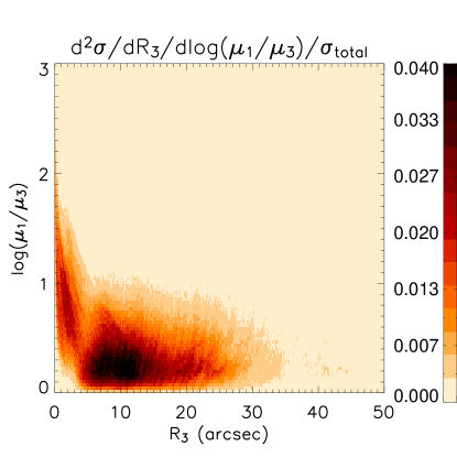
Figure 8: The top shows the normalised differential cross-section for three-image systems in the parameter space of $\log\mu_{1}/\mu_{3}$ and $R_{3}$ for the $\Lambda{\rm CDM}$0 cosmology, here $R_{3}$ is the separation of the central image relative to the cluster centre, $\mu_{1}$ and $\mu_{3}$ are magnifications for the brightest and faintest images; the latter is taken as the central image. The cluster is at $z_{\rm l}=0.5$ and the source is at $z_{\rm s}=2.5$. The bottom left panel shows the differential probability distribution of $\log\mu_{1}/\mu_{3}$. The hatched region shows the corresponding cross-section for two-image systems, i.e., three-image systems with an infinitely de-magnified central image due to the BCG. The bottom right panel shows the probability distribution of $R_{3}$. The cumulative distribution is shown as the dashed line.

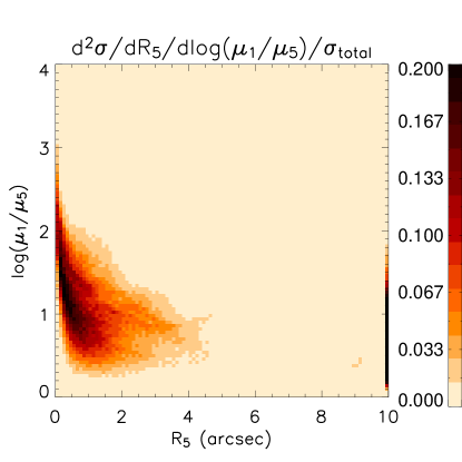
Figure 9: The top panel shows the normalised differential cross-section for five-image systems in the parameter space of $\log\mu_{1}/\mu_{5}$ and $R_{5}$ for the $\Lambda{\rm CDM}$0 cosmology, here $R_{5}$ is the separation of the central image relative to the cluster centre, and $\mu_{1}$ and $\mu_{5}$ are the magnifications of the brightest and faintest images respectively, the latter is taken as the central image. Systems with $R_{5}>10\arcsec$ have been collected at the right edge pixels. The bottom left panel shows the probability distribution of $\log\mu_{1}/\mu_{5}$, which is simply obtained by integrating the left panel along the $x$-axis. The integration ranges are from 0 to $5\arcsec$ for the dashed lines and from 0 to $\infty$ for the solid lines. The hatched region shows the corresponding cross-section for four-image systems, i.e., five-image systems with an infinitely de-magnified central image due to the BCG. The bottom right panel shows the probability distribution of $R_{5}$. The cumulative distribution is shown as the dashed line.

Of particular interests are the central images in systems with at least four images, because for the first cluster quasar lens, J1004+4112, subsequent deep imaging reveals a faint central image, at about 0.3% of the brightest image in the system (see Table 1 in Inada et al. 2005). The top panel of Fig. 9 shows the number of five-image systems in the plane of $\log\mu_{1}/\mu_{5}$, where $\mu_{5}$ is the magnification of the faintest image, and $R_{5}$ is the distance of this image from the cluster centre. There are also five-image systems with $R_{5}>10\arcsec$; they have been plotted in the right-edge pixels in the left panel.

If we marginalise the separation from the cluster centre, we obtain the probability distribution of magnification ratio, $\mu_{1}/\mu_{5}$, shown in the bottom left panel of Fig. 9. The solid line includes only those five-image systems with $R_{5}<5\arcsec$ while the dashed line includes all five-image systems. The solid line excludes most systems produced by merging sub-clusters. From these curves alone it seems that there is only a small probability of obtaining the magnification ratio of 300, the observed value for J1004+4112. In fact, only 3% will have a central image be fainter than the brightest one by a factor of 100. However, this discounts those four-image systems where the central image has disappeared. The hatched region is for those four image systems where the central image has been infinitely de-magnified by the BCG. The total cross-section for such systems is in fact quite large, about a factor of two of that for five-image systems. If we regard all these four-image systems as five-image systems with infinitely demagnified central images, the fraction will increase to $\sim(0.03+2)/(1+2)\sim 68\%$. If the profile is slightly shallower than the isothermal slope, $\rho\propto r^{-2}$, these central images will have a very small but finite magnification. Such central images may be what we are seeing in J1004+4112. Clearly the brightness of the central image will be a very sensitive probe of the central density profiles of BCGs.

The bottom right panel of Fig. 9 shows the distribution of $R_{5}$. It can be seen that, roughly 50 per cent of five-image systems have separation from the cluster centre smaller than $1.5\arcsec$. About 25% have separation larger than $5\arcsec$, these are due to five-image systems produced by merging sub-clusters. If we include four-image systems, and assume all the infinitely demagnified central images have $R_{5}<1.5\arcsec$, then the vast majority ($\sim(0.5+2)/(1+2)\sim 80\%$) of these systems will have central images within $1.5\arcsec$ of the BCG. These properties are broadly consistent with the observed system J1004+4112.

4.4 Cosmic variance

Figure 10: Top panel: the solid and dashed histograms show the mass functions at redshift 0.5 in our $\Lambda{\rm CDM}0$ and WMAP3 simulations respectively. The solid and dashed curves are the Sheth & Tormen (2002) mass functions. The two bottom panels show the differential cross-sections as a function of the logarithm of the cluster mass in the two models. The total area under each curve is normalised to unity. The clusters are at redshift 0.5 and the sources are at redshift 2.5. One can see that the box size of $\Lambda{\rm CDM}$0 simulation is large enough to sample the massive clusters but our WMAP3 simulation does not appear to have converged in the cross-section as a function of the cluster mass.

Our two simulations were run with a box size of $300h^{-1}\,\rm Mpc$. A question naturally arises is whether they sample the mass functions well, especially for the high-mass end in the WMAP3 model, and how much our results are affected by the cosmic variance. The top panel in Fig. 10 shows the mass functions in our simulations. The solid and dashed histograms are the mass functions at redshift 0.5 in our $\Lambda{\rm CDM}$0 and WMAP3 simulations respectively. The solid and dashed curves are the theoretical Sheth & Tormen (2002) mass functions, which is based on the Press-Schechter (1974) formalism and the ellipsoidal collapse model (Sheth, Mo & Tormen 2001). We can see that the number density of halos in the WMAP3 model is always smaller than that in the $\Lambda{\rm CDM}$0 model on cluster mass scale. For $M\sim 10^{14}h^{-1}M_{\odot}$, the abundance of halos is lower by a factor of 3.1 in the WMAP3 model compared with that in the $\Lambda{\rm CDM}$0 model; for $M\sim 10^{15}h^{-1}M_{\odot}$, the reduction factor is $\sim 8.8$. The number density in the last bin of the WMAP3 mass function is higher than prediction by a factor of $\sim$ 6 due to the presence of just 6 clusters. The low number of clusters at the high mass end in the WMAP3 model implies that ideally a larger simulation box is required to sample at least a similar number of massive clusters as in the $\Lambda{\rm CDM}$0 model. The two bottom panels show the differential cross-section as a function of the cluster mass in the two simulations. The total area under each curve is normalised to unity. The clusters are at redshift 0.5 and the sources are at redshift 2.5.

The mass distribution of SDSS J1004+4112 was studied in Ota et al. (2006) using X-ray data. Assuming isothermality and an NFW profile for the cluster, the virial mass was derived to be $M\sim 4.2^{+2.6}_{-1.5}\times 10^{14}h^{-1}M_{\odot}$. The mass of SDSS J1029+2623 is more uncertain. The image separation implies a cluster velocity dispersion $\sigma\sim\rm 900km/s$ (see Inada et al. 2006), and this can be converted to $M\sim 5.6\times 10^{14}h^{-1}M_{\odot}$ using cluster scaling relations, but with a large error bar. The box size of $\Lambda{\rm CDM}$0 simulation appears to be large enough to produce such massive clusters easily. On the other hand, there are only  20 clusters in the last three bins in the bottom-right panel of Fig. 10, such a small number may be not sufficiently sample the clusters well in the mass-concentration space and result in a relatively large errors of differential cross-section at the very high-mass end. But the final optical depth is the integration of the mean cross-section as a function of redshift, which will suppress the final variance. However our WMAP3 simulation does suffer seriously from the cosmic variance and appears to have too many very massive clusters compared to the theoretical prediction. In Li et al. (2006b), we ran a lower resolution simulation in the WMAP3 model which evolves $N_{\rm DM}=512^{3}$ dark matter particles in a box with sidelength of $600h^{-1}\,\rm Mpc$. Due to the larger volume, that simulation better samples the high mass tail of the cluster mass function and merger events. Comparing these simulations, we found that the smaller simulation over-estimates the number of giant arcs by a factor of 2. For the same reason, the number of wide-separation lensed quasars in the WMAP3 may be over-estimated by a similar factor. The WMAP3 cosmology is compatible with observations only at $\sim 4\%$ and $\sim 2\%$ level for an over-estimation by a factor of 1.5 and 2 respectively. However, we caution that to more properly account for the cosmic variance, it is necessary to run a much larger simulation with high resolutions in order to sample the cluster mass function sufficiently.

5 Summary and Discussions

In this paper, we have considered the number of multiply-imaged quasars lensed by clusters of galaxies in the SDSS photometric and spectroscopic quasar samples. A similar, earlier attempt was made by Hennawi et al. (2007b). This study extends their study by exploring how the predictions depend on the cosmology. We also study the multiply-imaged quasars as a function of image multiplicity, and explored in some detail the properties of central images. Our main conclusions are as follows

1. We found that the predicted multiply-imaged quasars with separation $>10\arcsec$ in the SDSS photometric sample (with an effective area 8000 deg²) is about 6.2, and about 2.6 in the spectroscopic sample (with an effective area 5000 deg²) in $\Lambda{\rm CDM}$0 model. These numbers are reduced by a factor of $\sim$7 or more in the WMAP3 model.

2. The predicted cluster lens peaks around redshift 0.5, and 90% are between 0.2 and 1. This distribution is largely independent of cosmology, and similar for both the photometric and spectroscopic samples.

3. The relative number of systems with ${N_{\rm img}}\geq 4$ images and those with ${N_{\rm img}}\geq 2$ images is about 1/3.5. This ratio is largely cosmology independent, and similar for both the photometric and spectroscopic quasar samples.

4. Because we modelled the BCGs as a truncated isothermal sphere, this creates a region, comparable in size to the angular Einstein radius of the BCG, inside which the central image disappears. For most central images in five-image configurations are quite faint, and close to the cluster centres. For three-image systems, the central images are brighter and further away from the cluster centres.

One uncertainty in our calculation is the ad hoc inclusion of a BCG at the centres of clusters at all redshifts. In reality, the BCGs are assembled as a function of time, and so it is interesting to estimate the effects of an evolving population of BCGs. We adopt a simple model by assuming there are no BCGs at the centres of clusters above redshift 0.5. Hennawi et al. (2007) finds that the optical depth decreases by a factor of 1/3 if all the BCGs are ignored. However, from Fig. 6, the contribution of clusters with $z_{\rm l}\ga 0.5$ is about 1/2 of the total cross-section. Thus if we remove all the BCGs from the clusters above redshift 0.5, the optical depth will decrease roughly by $\sim 16\%$. So the evolution effect may be modest. In any case, such a decrease in the optical depth will make the match between the WMAP3 model and the observations slightly worse.

Our predicted numbers of multiply-imaged quasars for both the photometric and spectroscopic samples are lower than those by Hennawi et al. (2007b) roughly by a factor of 2 in the $\Lambda{\rm CDM}$0 cosmology. Part of this difference is due to the slightly higher $\sigma_{8}$ (0.95) adopted by Hennawi et al. (2007b). The abundance for typical lensing clusters around $M>10^{14.5}h^{-1}M_{\odot}$ at redshift 0.5 is about 30% higher than that in our model with $\sigma_{8}=0.9$. Their higher $\sigma_{8}$ not only provides more massive clusters but also makes the cluster formation earlier and with higher concentration; both may increase the predicted number of cluster lenses. Our quasar luminosity function is similar to those adopted in Hennawi et al. (2007b) for the low redshift intervals, but is a factor of 2 higher than that adopted in their paper for the high-redshift interval ($z_{\rm s}\sim 4$). So the difference in the source luminosity function goes in the opposite direction. Note, however, the number of such higher redshift quasars is small and so this should not impact significantly on the overall predicted large-separation lenses (see Fig. 7).

For galaxy-scale lenses, the number of lenses with ${N_{\rm img}}\geq 4$ is about one half of that with ${N_{\rm img}}\geq 2$. For example, the statistical sample of the Cosmic Lens All Sky Survey (CLASS) has 13 lenses, 6 have at least 4 images (including one with 6 images, Browne et al. 2003; Chae 2003). Our study indicates the ratio is about 0.3 for cluster-scale lenses, about a factor of 1.5 smaller. This is consistent with Oguri & Keeton (2004). Using a triaxial cluster model, they found the ratio is 0.2 for inner density profile $\alpha=1$ and 0.4 for $\alpha=1.5$. The comparison between the two studies is, however, not straightforward as we use different definitions of $N_{\rm img}$ and their study also all of the faintest images in the multiply imaged systems can be detected, while in our study we assume certain magnitude limits for the images to be observable (see §3.1). If we relax the magnitude limit to $i=25$, then we find that our ratio is changed to 0.35, still within the bracket of the two values of Oguri & Keeton (2004) for different inner density slopes. As discussed by Rusin & Tegmark (2001) and Oguri & Keeton (2004), this ratio depends on a number of parameters, including the shape of the lensing potential and the density slopes. It appears that this is mainly because of the shallower inner density slope which causes the factor of 1.5 difference in the relative numbers between cluster lenses and galaxy lenses.

One striking result of this study is the reduction in the predicted number of large-separation lenses in the WMAP3 model compared with that in the $\Lambda{\rm CDM}$0 model. This reduction is comparable to that for the giant arcs ($\sim 6$) in these two cosmologies. However, we emphasise that the uncertainty for the quasar sample is smaller, because the source population is reasonably well known (see §3). There are two lens systems, J0114+4112 and J1029+2623, have been discovered in the SDSS spectroscopic sample with an effective area of $\sim 6500$deg². In the $\Lambda{\rm CDM}$0 model, from Fig. 5, the number of lenses with separation larger than $14.6\arcsec$ quadrupole-images and $22.5\arcsec$ double images are 0.7 and 1.2. This is roughly consistent with what we have discovered in the SDSS. However, for the WMAP3 model, the number of lenses with separation larger than $14.6\arcsec$ quadrupole-images and $22.5\arcsec$ double images are 0.09 and 0.14 for the whole spectroscopic sample. Assuming a Poisson distribution, the probability to observe two quasar systems in the WMAP3 model is $\sim$ 8% and decreases to 4% or lower if we account for the cosmic variance in our simulation (see §4.4). So it appears that a higher $\sigma_{8}$ or a higher $\Omega_{\rm m,0}$ is preferred by the data.

Clearly it is desirable to have a much bigger sample of large-separation multiply-imaged quasars. Our study shows that most cluster lenses have already been discovered in the SDSS spectroscopic quasar sample, but several more candidates may yet to be discovered in the photometric sample. Future large surveys may discover many more such examples (Wittman et al. 2006), which will provide strong constraints on the cosmology and the central mass profiles of clusters of galaxies.

References

- Boyle et al. (2000) Boyle B. J., Shanks T., Croom S. M., Smith R. J., Miller L., Loaring N., Heymans C., 2000, MNRAS, 317,1014
- Bowman et al. (2004) Bowman J. D., Hewitt J. N., Kiger J. R., 2004, ApJ, 617, 81
- Bryan & Norman (1998) Bryan G. L., Norman M. L., 1998, ApJ, 495, 80
- Browne et al. (2003) Browne I. W. B., et al. 2003, MNRAS, 341, 13
- Burke (1981) Burke W. L., 1981, ApJ, 244, L1
- Chae (2003) Chae K. H., 2003, MNRAS, 346, 746
- Chen (2004) Chen D. M., 2004, A&A, 418, 387
- Dalal et al. (2004) Dalal, N. Holder G., Hennawi J. F., 2004, ApJ, 609, 50
- Comerford et al. (2006) Comerford J. M., Meneghetti M., Bartelmann M., Schirmer M., 2006, ApJ, 642, 39
- Fontanot et al (2006) Fontanot F., Cristiani S., Monaco P., Nonino M., Vanzella E., Brandt W. N., Grazian A., Mao J., 2006, A&A, 461, 39
- Gladders et al. (2003) Gladders M. D., Hoekstra H., Yee H. K. C., Hall P. B., Barrientos L. F., 2003, ApJ, 593, 48
- Hennawi et al. (2006) Hennawi J. F., et al. 2006, in press (astro-ph/0610061)
- Hennawi et al. (2007a) Hennawi, J. F. Dalal N., Bode P., Ostriker J. P., 2007a, ApJ, 654, 714
- Hennawi et al. (2007b) Hennawi J. F., Dalal N., Bode P., 2007b, ApJ, 654, 93
- Horesh et al. (2005) Horesh A., Ofek E. O., Maoz D., Bartelmann M., Meneghetti M., Rix H.W., 2005, ApJ, 633, 768
- Hogg et al. (2002) Hogg D. W., Baldry I. K., Blanton M. R., Eisenstein D. J., 2002, in press (astro-ph/0210394)
- Huterer & Ma (2004) Huterer D., Ma, C., 2004, ApJ, 600, L7
- Inada et al. (2003) Inada N., et al. 2003, Nature, 426, 810
- Inada et al. (2005) Inada N., et al. 2005, PASJ, 57, 7
- Inada et al. (2006) Inada N., et al. 2006, ApJ, 653, L97
- Jing & Suto (2002) Jing Y. P., Suto Y., 2002, ApJ, 574, 538
- Keeton & Madau (2001) Keeton C. R., Madau, P., 2001, ApJ, 549, L25
- Keeton (2003) Keeton C. R., 2003, ApJ, 582, 17
- Kitayama & Suto (1996) Kitayama T., Suto, Y., 1996, MNRAS, 280, 638
- Kochanek 2006 (2006) Kochanek C. S., Schneider P., Wambsganss J., “Gravitational Lensing: Strong, Weak & Micro”, Proceedings of the 33rd Saas-Fee Advanced Course; G. Meylan, P. Jetzer, P. North, eds. (Springer-Verlag, Heidelberg)
- (26) Kuhlen M., Keeton C. R., Madau P., 2004, ApJ, 601, 104
- Li & Ostriker (2002) Li L., Ostriker J. P., 2002, ApJ, 566, 652
- Li & Ostriker (2003) Li L., Ostriker J. P., 2003, ApJ, 595, 603
- Li et al. (2005) Li G. L., Mao S., Jing Y. P., Bartelmann M., Kang X., Meneghetti M., 2005, ApJ, 635, 795
- Li et al. (2006a) Li G. L., Mao S., Jing Y. P., Kang X., Bartelmann M., 2006a, ApJ, 652, 43
- Li et al. (2006b) Li G. L., Mao S., Jing Y. P., Mo H. J., Gao L., Lin W. P., 2006b, MNRAS, 372, L73
- Lopes & Miller (2004) Lopes A. M., Miller L., 2004, MNRAS, 348, 519
- Luppino et al. (1999) Luppino G. A., Gioia I. M., Hammer F., Le Fvre O., Annis J. A., 1999, A&AS, 136, 117
- Mao et al. (2001) Mao S., Witt H. J., Koopmans L. V. E., 2001, MNRAS, 323, 301
- Maoz et al. (1997) Maoz D., Rix H. W., Gal-Yam A., Gould A., 1997, ApJ, 486, 75
- Meneghetti et al. (2003a) Meneghetti M., Bartelmann M., Moscardini L., 2003a, MNRAS, 340, 105
- Meneghetti et al. (2003b) Meneghetti M., Bartelmann M., Moscardini L., 2003b, MNRAS, 346, 67
- Narasimha et al. (1986) Narasimha D., Subramanian K., Chitre S. M., 1986, Nature, 321, 45
- Ofek et al. (2001) Ofek E. O., Maoz D., Prada F., Kolatt T., Rix, H. W., 2001, MNRAS, 324, 463
- Oguri (2003) Oguri M., 2003, MNRAS, 339, L23
- Oguri et al. (2003) Oguri M., Lee J., Suto Y., 2003, ApJ, 599, 7
- Oguri et al. (2004) Oguri M., et al. 2004, ApJ, 605, 78
- Oguri & Keeton (2004) Oguri M., Keeton C. R., 2004, ApJ, 610, 663
- Ota et al. (2006) Ota N., et al. 2006, ApJ, 647, 215
- Phillips et al. (2001a) Phillips P. M., et al. 2001a, MNRAS, 328, 1001
- Phillips et al. (2001b) Phillips P. M., Browne I. W., Wilkinson P. N., 2001b, MNRAS, 321, 187
- Press & Schechter (1974) Press W. H., Schechter P., 1974, ApJ, 187, 425
- Richards et al. (2004) Richards G. T., et al. 2004, ApJS, 155, 257
- Richards et al. (2005) Richards G. T., et al. 2005, MNRAS, 360, 839
- Richards et al. (2006) Richards G. T., et al. 2006, AJ, 131, 2766
- Rusin & Tegmark (2001) Rusin D., Tegmark M., 2001, ApJ, 553, 709
- Rusin (2002) Rusin D., 2002, ApJ, 572, 705
- Rusin et al. (2005) Rusin D., Keeton C. R., Winn J. N., 2005, ApJ, 627, L93
- Sand et al. (2005) Sand D. J., True T., Ellis R. S., Smith G. P., 2005, ApJ, 627, 32
- Sarbu et al. (2001) Sarbu N., Rusin D., Ma C., 2001, ApJ, 561, L147
- Schneider et al. (2005) Schneider D. P., et al. 2005, AJ, 130, 367
- Seljak & Zaldarriaga (1996) Seljak U., Zaldarriaga M., 1996, ApJ, 469, 437
- Sharon et al. (2005) Sharon K., et al. 2005, ApJ, 629, L73
- Sheth & Tormen (2002) Sheth R. K., Tormen G., 2002, MNRAS, 329, 61
- Sheth, Mo & Tormen (2001) Sheth R. K., Mo H. J., Tormen G., 2001, MNRAS, 323, 1
- Spergel et al. (2006) Spergel D. N., et al. 2006, preprint (astro-ph/0603449)
- Springel, Yoshida, & White (2001) Springel V., Yoshida N., White S. D. M., 2001, NewA, 6, 79
- Springel (2005) Springel V., 2005, MNRAS, 364, 1105
- Torri et al. (2004) Torri E., Meneghetti M., Bartelmann M., Moscardini L., Rasia E., Tormen G., 2004, MNRAS, 349, 476
- Turner (1980) Turner E. L., 1980, ApJ, 242, L135
- van de Marel et al. (2000) van de Marel R. P., Magorrian J., Carlberg R. G., Yee H. K. C., Ellingson E., 2000, AJ, 119, 2038
- Voigt & Fabian (2006) Voigt L. M., Fabian A. C., 2006, MNRAS, 368, 518
- Wambsganss et al. (2004) Wambsganss J., Bode P., Ostriker J. P., 2004, ApJ, 606, L93
- Winn et al. (2003) Winn J. N., Rusin D., Kochanek C. S., 2003, ApJ, 587, 80
- Winn et al. (2004) Winn J. N., Rusin D., Kochanek C. S., 2004, Nature, 427, 613
- Wittman et al. (2006) Wittman D., Dell’Antonio I. P., Hughes J. P., Margoniner V. E., Tyson J. A., Cohen J. G., Norman D., 2006, ApJ, 643, 128
- Wyithe et al. (2001) Wyithe J. S. B., Turner E. L., Spergel D. N., 2001, ApJ, 555, 504
- Zaritsky & Gonzalez (2003) Zaritsky D., Gonzalez A. H., 2003, ApJ, 584, 691