A Simple and Accurate Riemann Solver for Isothermal MHD

Abstract

A new approximate Riemann solver for the equations of magnetohydrodynamics (MHD) with an isothermal equation of state is presented. The proposed method of solution draws on the recent work of Miyoshi and Kusano, in the context of adiabatic MHD, where an approximate solution to the Riemann problem is sought in terms of an average constant velocity and total pressure across the Riemann fan. This allows the formation of four intermediate states enclosed by two outermost fast discontinuities and separated by two rotational waves and an entropy mode. In the present work, a corresponding derivation for the isothermal MHD equations is presented. It is found that the absence of the entropy mode leads to a different formulation which is based on a three-state representation rather than four. Numerical tests in one and two dimensions demonstrates that the new solver is robust and comparable in accuracy to the more expensive linearized solver of Roe, although considerably faster.

1 Introduction

The numerical solution of the magnetohydrodynamics (MHD) equations has received an increasing amount of attention over the last few decades motivated by the growing interests in modeling highly nonlinear flows. Numerical algorithms based on upwind differencing techniques have established stable and robust frameworks for their ability to capture the dynamics of strong discontinuities. This success owes to the proper computation of numerical fluxes at cell boundaries, based on the solution of one-dimensional Riemann problems between adjacent discontinuous states. The accuracy and strength of a Riemann solver is intrinsically tied to the degree of approximation used in capturing the correct wave pattern solution.

In the case of adiabatic flows, an arbitrary initial discontinuity evolves into a pattern of constant states separated by seven waves, two pairs of magneto-sonic waves (fast and slow), two Alfvén discontinuities and one contact or entropy mode. With the exception of the entropy mode, a wave separating two adjacent states may be either a shock or a rarefaction wave. In the limit of efficient radiative cooling processes or highly conducting plasma, on the other hand, the adiabatic assumption becomes inadequate and the approximation of an isothermal flow is better suited to describe the flow. In this case, the solution of the Riemann problem is similar to the adiabatic case, with the exception of the contact mode which is absent.

Although analytical solutions can be found with a high degree of accuracy using exact Riemann solvers, the resulting numerical codes are time-consuming and this has pushed researcher’s attention toward other more efficient strategies of solution. From this perspective, a flourishing number of approaches has been developed in the context of adiabatic MHD, see for example [DW, 14, 5, Balsara] and references therein. Similar achievements have been obtained for the isothermal MHD equations, see [Balsara, 13].

Recently, Miyoshi and Kusano ([12], MK henceforth) proposed a multi-state Harten-Lax-van Leer (HLL, [11]) Riemann solver for adiabatic MHD. The proposed “HLLD” solver relies on the approximate assumption of constant velocity and total pressure over the Riemann fan. This naturally leads to a four-state representation of the solution where fast, rotational and entropy waves are allowed to form. The resulting scheme was shown to be robust and accurate. The purpose of the present work is to extend the approach developed by MK to the equations of isothermal magnetohydrodynamics (IMHD henceforth). Although adiabatic codes with specific heat ratios close to one may closely emulate the isothermal behavior, it is nevertheless advisable to develop codes specifically designed for IMHD, because of the greater ease of implementation and efficiency over adiabatic ones.

The paper is structured as follows: in §2 the equations of IMHD are given; in §3 the new Riemann solver is derived. Numerical tests are presented in §4 and conclusions are drawn in §5.

2 Governing Equations

The ideal MHD equations describing an electrically conducting perfect fluid are expressed by conservation of mass,

$$\frac{\partial\rho}{\partial t}+\nabla\cdot(\rho\mathbf{v})=0\,,$$ (1)

momentum,

$$\frac{\partial\mathbf{m}}{\partial t}+\nabla\cdot\left(\mathbf{m}\mathbf{v}-\mathbf{B}\mathbf{B}+\mathbf{I}p_{T}\right)=0\,,$$ (2)

and magnetic flux,

$$\frac{\partial\mathbf{B}}{\partial t}-\nabla\times\left(\mathbf{v}\times\mathbf{B}\right)=0\,.$$ (3)

The system of equations is complemented by the additional solenoidal constraint $\nabla\cdot\mathbf{B}=0$ and by an equation of state relating pressure, internal energy and density and Here $\rho$, $\mathbf{v}$ and $\mathbf{m}=\rho\mathbf{v}$ are used to denote, respectively, density, velocity and momentum density. The total pressure, $p_{T}$, includes thermal ($p$) and magnetic ($|\mathbf{B}|^{2}/2$) contributions (a factor of $\sqrt{4\pi}$ has been reabsorbed in the definition of $\mathbf{B}$). No energy equation is present since I will consider the isothermal limit for which one has $p=a^{2}\rho$, where $a$ is the (constant) isothermal speed of sound. With this assumption the total pressure can be written as:

$$p_{T}=a^{2}\rho+\frac{|\mathbf{B}|^{2}}{2}\,.$$ (4)

Finite volume numerical schemes aimed to solved (1)–(3) rely on the solution of one-dimensional Riemann problems between discontinuous left and right states at zone edges. Hence without loss of generality, I will focus, in what follows, on the one-dimensional hyperbolic conservation law

$$\frac{\partial\mathbf{U}}{\partial t}+\frac{\partial\mathbf{F}}{\partial x}=0\,,$$ (5)

where the vector of conservative variables $\mathbf{U}$ and the corresponding fluxes $\mathbf{F}$ are given by

$$\mathbf{U}=\left(\begin{array}[]{c}\rho\\ \vskip 6.0pt plus 2.0pt minus 2.0pt\cr\rho u\\ \vskip 6.0pt plus 2.0pt minus 2.0pt\cr\rho v\\ \vskip 6.0pt plus 2.0pt minus 2.0pt\cr\rho w\\ \vskip 6.0pt plus 2.0pt minus 2.0pt\cr B_{y}\\ \vskip 6.0pt plus 2.0pt minus 2.0pt\cr B_{z}\end{array}\right)\,,\quad\mathbf{F}=\left(\begin{array}[]{c}\rho u\\ \vskip 6.0pt plus 2.0pt minus 2.0pt\cr\rho u^{2}+p_{T}-B_{x}^{2}\\ \vskip 6.0pt plus 2.0pt minus 2.0pt\cr\rho vu-B_{x}B_{y}\\ \vskip 6.0pt plus 2.0pt minus 2.0pt\cr\rho wu-B_{x}B_{z}\\ \vskip 6.0pt plus 2.0pt minus 2.0pt\cr B_{y}u-B_{x}v\\ \vskip 6.0pt plus 2.0pt minus 2.0pt\cr B_{z}u-B_{x}w\end{array}\right)\,,$$ (6)

where $u,v$ and $w$ are the three components of velocity in the $x$, $y$ and $z$ directions, respectively. The solution of Eq. (5) may be achieved through the standard two-point finite difference scheme

$$\mathbf{U}_{i}^{n+1}=\mathbf{U}_{i}^{n}-\frac{\Delta t}{\Delta x}\left(\hat{\mathbf{F}}_{i+\frac{1}{2}}-\hat{\mathbf{F}}_{i-\frac{1}{2}}\right)\,,$$ (7)

where $\hat{\mathbf{F}}_{i\pm\frac{1}{2}}$ is the numerical flux function, properly computed by solving a Riemann problem between $\mathbf{U}_{i}$ and $\mathbf{U}_{i\pm 1}$.

As already mentioned, the solution to the Riemann problem in IMHD consists of a six wave pattern, with two pairs of magneto-sonic waves (fast and slow) and two Alfvén (rotational) waves. These families of waves propagate information with characteristic signal velocities given by the eigenvalues of the Jacobian $\partial\mathbf{F}(\mathbf{U})/\partial\mathbf{U}$:

$$\lambda_{f_{\pm}}=u\pm c_{f}\,,\quad\lambda_{s_{\pm}}=u\pm c_{s}\,,\quad\lambda_{a_{\pm}}=u\pm c_{a}\,,\quad$$ (8)

where the fast, Alfvén and slow velocity are defined as in adiabatic MHD:

$$c_{f}=\left[\frac{1}{2}\left(a^{2}+\mathbf{b}^{2}+\sqrt{\left(a^{2}+\mathbf{b}^{2}\right)^{2}-4a^{2}b_{x}^{2}}\right)\right]^{1/2}\,,$$ (9)

$$c_{a}=|b_{x}|$$ (10)

$$c_{s}=\left[\frac{1}{2}\left(a^{2}+\mathbf{b}^{2}-\sqrt{\left(a^{2}+\mathbf{b}^{2}\right)^{2}-4a^{2}b_{x}^{2}}\right)\right]^{1/2}\,,$$ (11)

with $\mathbf{b}=\mathbf{B}/\sqrt{\rho}$.

The contact or entropy mode is absent. Fast and slow waves can be either shocks, where flow quantities experience a discontinuous jump, or rarefaction waves, characterized by a smooth transition of the state variables. Across the rotational waves, similarly to the adiabatic case, density and normal component of velocity are continuous, whereas tangential components are not. In virtue of the solenoidal constraint, the normal component of the magnetic field is constant everywhere and should be regarded as a given parameter.

3 The HLLD Approximate Riemann Solver

Figure 1: Schematic representation of the approximated wave structure used to describe the Riemann fan. The initial states $U_{L}$ and $U_{R}$ are connected to each other through a set of four waves ($S_{L}$, $S^{*}_{L}$ $S^{*}_{R}$ and $S_{R}$) across which some or all of the fluid variables can be discontinuous. The four discontinuities isolate three intermediate constant states $U^{*}_{L}$, $U^{*}_{c}$ and $U^{*}_{R}$ which correspond to the approximate solution of the Riemann problem.

In what follows, I will assume that the solution to the isothermal MHD Riemann problem can be represented in terms of three constant states, $\mathbf{U}^{*}_{L}$, $\mathbf{U}^{*}_{c}$ and $\mathbf{U}^{*}_{R}$, separated by four waves: two outermost fast magneto-sonic disturbances with speeds $S_{L}$ and $S_{R}$ ($S_{L}<S_{R}$) and two innermost rotational discontinuities with velocities $S^{*}_{L}$ and $S^{*}_{R}$, see Fig. 1. Slow modes cannot be generated inside the solution. Since no entropy mode is present and rotational discontinuities carry jumps in the tangential components of vector fields only, it follows that one can regard density, normal velocity and total pressure as constants over the fan. This assumption is essentially the same one suggested by MK but it leads, in the present context, to a representation in terms of three states rather than four. Quantities ahead and behind each wave must be related by the jump conditions

$$S_{\alpha}\left(\mathbf{U}^{*}_{\alpha}-\mathbf{U}_{\alpha}\right)=\mathbf{F}^{*}_{\alpha}-\mathbf{F}_{\alpha}\,,$$ (12)

across the outermost fast waves, and

$$S^{*}_{\alpha}\left(\mathbf{U}^{*}_{c}-\mathbf{U}^{*}_{\alpha}\right)=\mathbf{F}^{*}_{c}-\mathbf{F}^{*}_{\alpha}\,,$$ (13)

across the innermost Alfvén waves. Here $\alpha=L$ or $\alpha=R$ is used for the left or right state, respectively. Note that $\mathbf{U}^{*}$ and $\mathbf{F}^{*}$ are both unknowns of the problem and $\mathbf{F}^{*}$ should not be confused with $\mathbf{F}(\mathbf{U}^{*})$, although one always has $\mathbf{F}_{\alpha}=\mathbf{F}(\mathbf{U}_{\alpha})$.

The solution to the problem must satisfy the consistency condition which, in terms of $\mathbf{U}^{*}$, can be obtained by direct summation of Eq. (12) and (13) across all waves:

$$\frac{\left(S_{L}^{*}-S_{L}\right)\mathbf{U}^{*}_{L}+\left(S_{R}^{*}-S_{L}^{*}\right)\mathbf{U}^{*}_{c}+\left(S_{R}-S_{R}^{*}\right)\mathbf{U}^{*}_{R}}{S_{R}-S_{L}}=\mathbf{U}^{\rm hll}\,,$$ (14)

where

$$\mathbf{U}^{\rm hll}=\frac{S_{R}\mathbf{U}_{R}-S_{L}\mathbf{U}_{L}-\mathbf{F}_{R}+\mathbf{F}_{L}}{S_{R}-S_{L}}$$ (15)

is the HLL single average state. Likewise, after dividing Eq. (12) and (13) by $S_{\alpha}$ and $S^{*}_{\alpha}$ (respectively) and adding the resulting equations, the following condition for the fluxes $\mathbf{F}^{*}$ is found:

$$\frac{\left(\frac{1}{S^{*}_{L}}-\frac{1}{S_{L}}\right)\mathbf{F}^{*}_{L}+\left(\frac{1}{S_{R}^{*}}-\frac{1}{S_{L}^{*}}\right)\mathbf{F}^{*}_{c}+\left(\frac{1}{S_{L}^{*}}-\frac{1}{S_{R}^{*}}\right)\mathbf{F}^{*}_{R}}{\frac{1}{S_{R}}-\frac{1}{S_{L}}}=\mathbf{F}^{\rm hll}\,,$$ (16)

where

$$\mathbf{F}^{\rm hll}=\frac{S_{R}\mathbf{F}_{L}-S_{L}\mathbf{F}_{R}+S_{R}S_{L}(\mathbf{U}_{R}-\mathbf{U}_{L})}{S_{R}-S_{L}}$$ (17)

is the HLL single average flux. Equation (17) represents the average flux function inside the Riemann fan and can be considered as the “dual” relation of (15). Indeed, Eq. (17) could have been obtained by letting $\mathbf{U}_{\alpha}\to\mathbf{F}_{\alpha}$, $\mathbf{F}_{\alpha}\to\mathbf{U}_{\alpha}$ and $S_{\alpha}\to 1/S_{\alpha}$ on the right hand side of Eq. (15).

In this approximation, density, normal velocity and total pressure do not experience jumps across the inner waves and are constant throughout the Riemann fan, i.e., $\rho^{*}_{L}=\rho^{*}_{c}=\rho^{*}_{R}\equiv\rho^{*}$, $u^{*}_{L}=u^{*}_{c}=u^{*}_{R}\equiv u^{*}$, $p_{T_{L}}^{*}=p_{T_{c}}^{*}=p_{T_{R}}^{*}\equiv p^{*}_{T}$. Tangential components of magnetic field and velocity, on the other hand, may be discontinuous across any wave and their jumps must be computed using (12) or (13).

At first sight, one might be tempted to proceed as in the adiabatic case, that is, by writing $\mathbf{U}^{*}$ and $\mathbf{F}^{*}$ in terms of the seven unknowns $\rho^{*}$, $u^{*}$, $v^{*}$, $w^{*}$, $B_{y}^{*}$, $B_{z}^{*}$ and $p_{T}^{*}$, and then using Eq. (12) and (13), together with the continuity of $\rho^{*}$, $u^{*}$ and $p_{T}^{*}$, to determine the jumps accordingly. However, this approach is mathematically incorrect since the resulting system of equations is overdetermined. This can be better understood by explicitly writing the first and second component of Eq. (12):

$$S_{\alpha}\left(\rho^{*}-\rho_{\alpha}\right) = \rho^{*}u^{*}-\rho_{\alpha}u_{\alpha}\,,$$ (18)

$$S_{\alpha}\left(\rho^{*}u^{*}-\rho_{\alpha}u_{\alpha}\right) = \rho^{*}(u^{*})^{2}+p_{T}^{*}-\rho_{\alpha}u_{\alpha}-p_{T_{\alpha}}\,,$$ (19)

where I have used the fact the $\rho^{*}$, $u^{*}$ and $p^{*}_{T}$ are constants in each of the three states. Eqns (18) and (19) provide four equations (two for $\alpha=L$ and two for $\alpha=R$) in the three unknowns $\rho^{*}$, $u^{*}$ and $p^{*}_{T}$ and, as such, they cannot have a solution. Furthermore, the situation does not improve when the equations for the tangential components are included, since more unknowns are brought in.

The problem can be disentangled by writing density and momentum jump conditions in terms of four unknowns rather than three. This is justified by the fact that, according to the chosen representation, density and momentum components of $\mathbf{U}^{*}$ and $\mathbf{F}^{*}$ are continuous across the Riemann fan and, in line with the consistency condition, they should be represented by their HLL averages:

$$\rho^{*}\equiv\rho^{*}_{L}=\rho^{*}_{c}=\rho^{*}_{R}=\rho^{\rm hll}\,,$$ (20)

$$m_{x}^{*}\equiv m^{*}_{x_{L}}=m^{*}_{x_{c}}=m^{*}_{x_{R}}=m_{x}^{\rm hll}\,,$$ (21)

$$F^{*}_{[\rho]}\equiv F^{*}_{[\rho]_{L}}=F^{*}_{[\rho]_{c}}=F^{*}_{[\rho]_{R}}=F_{[\rho]}^{\rm hll}\,,$$ (22)

$$F^{*}_{[m_{x}]}\equiv F^{*}_{[m_{x}]L}=F^{*}_{[m_{x}]c}=F^{*}_{[m_{x}]R}=F^{\rm hll}_{[m_{x}]}\,,$$ (23)

where $\rho^{\rm hll}$, $m^{\rm hll}$, $F_{[\rho]}^{\rm hll}$ and $F^{\rm hll}_{[m_{x}]}$ are given by the first two components of Eq. (15) and Eq. (17).

This set of relations obviously satisfies the jump conditions across all the four waves. The absence of the entropy mode, however, leaves the velocity in the Riemann fan, $u^{*}$, unspecified. This is not the case in the adiabatic case, where one has $m^{*}=F^{*}_{[\rho]}=\rho^{*}u^{*}$ and from the analogous consistency condition the unique choice $\rho^{\rm hll}u^{*}=m_{x}^{\rm hll}$. Still, in the isothermal case, one has the freedom to define $u^{*}=F^{\rm hll}_{[\rho]}/\rho^{\rm hll}$ or $u^{*}=m_{x}^{\rm hll}/\rho^{\rm hll}$. The two choices are not equivalent and one can show that only the first one has the correct physical interpretation an “advective” velocity. This statement becomes noticeably true in the limit of vanishing magnetic fields, where transverse velocities are passively advected and thus carry zero jump across the outermost sound waves. Indeed, by explicitly writing the jump conditions for the transverse momenta, one can see that the conditions $v^{*}_{\alpha}=v_{\alpha}$ and $w^{*}_{\alpha}=w_{\alpha}$ can be fulfilled only if $\rho^{*}u^{*}=F^{*}_{[\rho]}$.

Thus one has, for variables and fluxes in the star region, the following representation:

$$\mathbf{U}^{*}=\left(\begin{array}[]{c}\rho^{*}\\ \vskip 6.0pt plus 2.0pt minus 2.0pt\cr m^{*}_{x}\\ \vskip 6.0pt plus 2.0pt minus 2.0pt\cr\rho^{*}v^{*}\\ \vskip 6.0pt plus 2.0pt minus 2.0pt\cr\rho^{*}w^{*}\\ \vskip 6.0pt plus 2.0pt minus 2.0pt\cr B^{*}_{y}\\ \vskip 6.0pt plus 2.0pt minus 2.0pt\cr B^{*}_{z}\end{array}\right)\,,\quad\mathbf{F}^{*}=\left(\begin{array}[]{c}\rho^{*}u^{*}\\ \vskip 6.0pt plus 2.0pt minus 2.0pt\cr F^{*}_{m_{x}}\\ \vskip 6.0pt plus 2.0pt minus 2.0pt\cr\rho^{*}v^{*}u^{*}-B_{x}B^{*}_{y}\\ \vskip 6.0pt plus 2.0pt minus 2.0pt\cr\rho^{*}w^{*}u^{*}-B_{x}B^{*}_{z}\\ \vskip 6.0pt plus 2.0pt minus 2.0pt\cr B^{*}_{y}u^{*}-B_{x}v^{*}\\ \vskip 6.0pt plus 2.0pt minus 2.0pt\cr B^{*}_{z}u^{*}-B_{x}w^{*}\end{array}\right)\,,$$ (24)

which gives $8$ variables per state and thus a total of $24$ unknowns. The 4 continuity relations (20)–(23) together with the 12 jump conditions (12) across the outer waves can be used to completely specify $\mathbf{U}^{*}_{\alpha}$ (for $\alpha=L$ and $\alpha=R$) in terms of $\mathbf{U}_{L}$ and $\mathbf{U}_{R}$. Note that the total pressure does not explicitly enter in the definition of the momentum flux. The remaining $4$ unknowns in the intermediate region ($v^{*}_{c}$, $w^{*}_{c}$, $B^{*}_{y_{c}}$ and $B^{*}_{z_{c}}$) may be found using (13). However, one can see that

$$(S^{*}_{\alpha}-u^{*})\rho^{*}v^{*}_{c}+B_{x}B^{*}_{y_{c}} = (S^{*}_{\alpha}-u^{*})\rho^{*}v^{*}_{\alpha}+B_{x}B^{*}_{y_{\alpha}}\,,$$ (25)

$$(S^{*}_{\alpha}-u^{*})\rho^{*}w^{*}_{c}+B_{x}B^{*}_{z_{c}} = (S^{*}_{\alpha}-u^{*})\rho^{*}w^{*}_{\alpha}+B_{x}B^{*}_{z_{\alpha}}\,,$$ (26)

$$(S^{*}_{\alpha}-u^{*})B^{*}_{y_{c}}+B_{x}v^{*}_{c} = (S^{*}_{\alpha}-u^{*})B^{*}_{y_{\alpha}}+B_{x}v^{*}_{\alpha}\,,$$ (27)

$$(S^{*}_{\alpha}-u^{*})B^{*}_{z_{c}}+B_{x}w^{*}_{c} = (S^{*}_{\alpha}-u^{*})B^{*}_{z_{\alpha}}+B_{x}w^{*}_{\alpha}\,,$$ (28)

cannot be simultaneously satisfied for $\alpha=L$ and $\alpha=R$ for an arbitrary definition of $S^{*}_{\alpha}$, unless the equations are linearly dependent, in which case one finds

$$S^{*}_{L}=u^{*}-\frac{|B_{x}|}{\sqrt{\rho^{*}}}\,,\quad S^{*}_{R}=u^{*}+\frac{|B_{x}|}{\sqrt{\rho^{*}}}\,.$$ (29)

This choice uniquely specifies the speed of the rotational discontinuity in terms of the average Alfvén velocity $|B_{x}|/\sqrt{\rho^{*}}$. Thus only $4$ (out of $8$) equations can be regarded independent and one has at disposal a total of $24$ independent equations, consistently with a well-posed problem.

Proceeding in the derivation, direct substitution of (24) into Eqns (12) together with (20), (29) and the assumption $u^{*}=F^{\rm hll}_{[\rho]}/\rho^{\rm hll}$ yields

$$\rho^{*}v^{*}_{\alpha}=\rho^{*}v_{\alpha}-B_{x}B_{y_{\alpha}}\frac{u^{*}-u_{\alpha}}{(S_{\alpha}-S^{*}_{L})(S_{\alpha}-S^{*}_{R})}\,,$$ (30)

$$\rho^{*}w^{*}_{\alpha}=\rho^{*}w_{\alpha}-B_{x}B_{z_{\alpha}}\frac{u^{*}-u_{\alpha}}{(S_{\alpha}-S^{*}_{L})(S_{\alpha}-S^{*}_{R})}\,,$$ (31)

$$B^{*}_{y_{\alpha}}=\frac{B_{y_{\alpha}}}{\rho^{*}}\frac{\rho_{\alpha}(S_{\alpha}-u_{\alpha})^{2}-B_{x}^{2}}{(S_{\alpha}-S^{*}_{L})(S_{\alpha}-S^{*}_{R})}\,,$$ (32)

$$B^{*}_{z_{\alpha}}=\frac{B_{z_{\alpha}}}{\rho^{*}}\frac{\rho_{\alpha}(S_{\alpha}-u_{\alpha})^{2}-B_{x}^{2}}{(S_{\alpha}-S^{*}_{L})(S_{\alpha}-S^{*}_{R})}\,,$$ (33)

which clearly shows that $(v^{*}_{\alpha},w^{*}_{\alpha})\to(v_{\alpha},w_{\alpha})$ when $\mathbf{B}\to\mathbf{0}$. As in the adiabatic case, the consistency condition should be used to find $v^{*}_{c}$, $w^{*}_{c}$, $B^{*}_{y_{c}}$ and $B^{*}_{z_{c}}$:

$$\rho^{*}v^{*}_{c} = \frac{(\rho^{*}v^{*}_{L}+\rho^{*}v^{*}_{R})}{2}+\frac{X(B^{*}_{y_{R}}-B^{*}_{y_{L}})}{2}\,,$$ (34)

$$\rho^{*}w^{*}_{c} = \frac{(\rho^{*}w^{*}_{L}+\rho^{*}w^{*}_{R})}{2}+\frac{X(B^{*}_{z_{R}}-B^{*}_{z_{L}})}{2}\,,$$ (35)

$$B^{*}_{y_{c}} = \frac{(B^{*}_{y_{L}}+B^{*}_{y_{R}})}{2}+\frac{(\rho^{*}v^{*}_{R}-\rho^{*}v^{*}_{L})}{2X}\,,$$ (36)

$$B^{*}_{z_{c}} = \frac{(B^{*}_{z_{L}}+B^{*}_{z_{R}})}{2}+\frac{(\rho^{*}w^{*}_{R}-\rho^{*}w^{*}_{L})}{2X}\,,$$ (37)

where $X=\sqrt{\rho^{*}}\textrm{sign}(B_{x})$. The inter-cell numerical flux $\hat{\mathbf{F}}$ required in Eq. (5) can now be computed by sampling the solution on the $x/t=0$ axis:

$$\hat{\mathbf{F}}=\left\{\begin{array}[]{ll}\mathbf{F}_{L}&\textrm{for}\quad S_{L}>0\\ \vskip 6.0pt plus 2.0pt minus 2.0pt\cr\mathbf{F}_{L}+S_{L}(\mathbf{U}^{*}_{L}-\mathbf{U}_{L})&\textrm{for}\quad S_{L}<0<S^{*}_{L}\\ \vskip 6.0pt plus 2.0pt minus 2.0pt\cr\mathbf{F}^{*}_{c}&\textrm{for}\quad S^{*}_{L}<0<S^{*}_{R}\\ \vskip 6.0pt plus 2.0pt minus 2.0pt\cr\mathbf{F}_{R}+S_{R}(\mathbf{U}^{*}_{R}-\mathbf{U}_{R})&\textrm{for}\quad S^{*}_{R}<0<S_{R}\\ \vskip 6.0pt plus 2.0pt minus 2.0pt\cr\mathbf{F}_{R}&\textrm{for}\quad S_{R}<0\\ \vskip 6.0pt plus 2.0pt minus 2.0pt\cr\end{array}\right.\,,$$ (38)

where $\mathbf{F}^{*}_{c}$ is computed from (24) using (34) through (37).

To conclude, one needs an estimate for the upper and lower signal velocities $S_{L}$ and $S_{R}$. I will adopt the simple estimate given by [8], for which one has

$$S_{L}=\min\left(\lambda_{f-}(\mathbf{U}_{L}),\lambda_{f-}(\mathbf{U}_{R})\right)\,,S_{R}=\min\left(\lambda_{f+}(\mathbf{U}_{L}),\lambda_{f+}(\mathbf{U}_{R})\right)\,,$$ (39)

with $\lambda_{f\pm}(\mathbf{U})$ given by the first of (8). Other estimates have been proposed, see for example [9].

The degenerate cases are handled as follows:

• for zero tangential components of the magnetic field and $B^{2}_{x}>a^{2}\rho_{\alpha}$, a degeneracy occurs where $S^{*}_{\alpha}\to S_{\alpha}$ and the denominator in Eqns. (30)–(33) vanishes. In this case, one proceeds as in the adiabatic case by imposing transverse components of velocity and magnetic field to have zero jump;

• the case $B_{x}\to 0$ does not poses any serious difficulty and only the states $\mathbf{U}^{*}_{L}$ and $\mathbf{U}^{*}_{R}$ have to be evaluated in order to compute the fluxes. One should realize, however, that the final representation of the solution differs from the adiabatic counterpart. In the full solution, in fact, Alfvén and slow modes all degenerate into a single intermediate tangential discontinuity with speed $u^{*}$. In the adiabatic case, this degeneracy can still be well described by the presence of the middle wave, across which only normal velocity and total pressure are continuous. Although this property is recovered by the adiabatic HLLD solver, the same does not occur in our formulation because of the initial assumption of constant density through the Riemann fan. The unresolved density jump, in fact, can be thought of as the limiting case of two slow shocks merging into a single wave. Since slow shocks are not considered in the solution, density will still be given by the single HLL-averaged state. Tangential components of velocity and magnetic field, on the other hand, can yet be discontinuous across the middle wave. Thus, in this limit, the solver does not reduce to the single state HLL solver.

This completes the description of the proposed isothermal HLLD Riemann solver. The suggested formulation satisfies the consistency conditions by construction and defines a well-posed problem, since the number of unknowns is perfectly balanced by the number of available equations: $12$ equations for the outermost waves, $8$ continuity conditions (for $\rho^{*}$, $u^{*}$, $F^{*}_{[\rho]}$, $F^{*}_{[m_{x}]}$ across the inner waves) and the $4$ equations for the tangential components. The positivity of the solver is trivial since no energy equation is present and the density is given by the HLL-averaged state (20).

4 Numerical Tests

The performance of the new Riemann solver is now investigated through a series of selected numerical tests in one and two dimensions. One dimensional shock tubes (in §4.1) consist in a decaying discontinuity initially separating two constant states. The outcoming wave pattern comprises several waves and an analytical or reference solution can usually be obtained with a high degree of accuracy. For this reason, one dimensional tests are commonly used to check the ability of the code in reproducing the correct structure.

The decay of standing Alfvén waves in two dimensions is consider in §4.2. The purpose of this test is to quantify the amount of intrinsic numerical dissipation inherent to a numerical scheme. A two dimensional tests involving the propagation of a blast wave in a strongly magnetized environment is investigated in §4.3 and finally, in §4.4, the isothermal Orszag-Tang vortex system and its transition to supersonic turbulence is discussed.

Eq. (7) is used for the spatially and temporally first order scheme. Extension to second order is achieved with the $2^{\rm nd}$ order fully unsplit Runge-Kutta Total Variation Diminishing (TVD) of [10] and the harmonic slope limiter of [17]. For the multidimensional tests, the magnetic field is evolved using the constrained transport method of [4], where staggered magnetic fields are updated, e.g. during the predictor step, according to

$$B^{n+1}_{x,i+\frac{1}{2},j} = B^{n}_{x,i+\frac{1}{2},j}-\frac{\Delta t}{\Delta y_{j}}\left(\Omega^{z}_{i+\frac{1}{2},j+\frac{1}{2}}-\Omega^{z}_{i+\frac{1}{2},j-\frac{1}{2}}\right)\,,$$ (40)

$$B^{n+1}_{y,i,j+\frac{1}{2}} = B^{n}_{y,i,j+\frac{1}{2}}+\frac{\Delta t}{\Delta x_{i}}\left(\Omega^{z}_{i+\frac{1}{2},j+\frac{1}{2}}-\Omega^{z}_{i-\frac{1}{2},j+\frac{1}{2}}\right)\,.$$ (41)

The electric field $\Omega^{z}_{i+\frac{1}{2},j+\frac{1}{2}}$ is computed by a spatial average the upwind fluxes available at zone interfaces during the Riemann solver step:

$$\Omega^{z}_{i+\frac{1}{2},j+\frac{1}{2}}=\frac{-\hat{F}^{[B_{y}]}_{i+\frac{1}{2},j}-\hat{F}^{[B_{y}]}_{i+\frac{1}{2},j+1}+\hat{F}^{[B_{x}]}_{i,j+\frac{1}{2}}+\hat{F}^{[B_{x}]}_{i+1,j+\frac{1}{2}}}{4}\,,$$ (42)

where $\hat{F}^{[B_{y}]}$ is the $B_{y}$ component of the flux (38) available during the sweep along the x-direction. A similar procedure applies to $\hat{F}^{[B_{x}]}$.

4.1 One Dimensional Shock Tubes

Test	$\rho$	$u$	$v$	$w$	$H_{x}$	$H_{y}$	$H_{z}$	$t_{s}$
1L	1	0	0	0	3	5	0	0.1
1R	0.1	0	0	0	3	2	0	-
2L	1.08	1.2	0.01	0.5	2	3.6	2	0.2
2R	1	0	0	0	2	4	2	-
3L	0.1	5	0	0	0	-1	-2	0.25
3R	0.1	-5	0	0	0	1	2	-

Table 1: Initial conditions for the one-dimensional shock tube problems presented in the text. Here $(H_{x},H_{y},H_{z})=\sqrt{4\pi}(B_{x},B_{y},B_{z})$. The final integration time ($t_{s}$) is given in the last column.

An interface separating two constant states is placed in the middle of the domain $[0,1]$ at $x=0.5$. Unless otherwise stated, the isothermal speed of sound $a$ is set to unity. States to the left and to the right of the discontinuity together with the final integration time are given in Table 1. The reader may also refer to [13] for the first and second problems and to [3] for the third one. For the sake of comparison, the linearized Riemann solver of Roe (properly adapted to the isothermal case from [5]) and the simple single-state HLL solver of [11] will also be used in the computations. In order to better highlight the differences between the selected Riemann solvers, integrations are carried with a spatially and temporally first order-accurate scheme on $400$ uniform zones. The Courant number is set to $0.8$ in all calculations.

Figure 2: Computed profiles for the first shock tube problem at time $t=0.1$. The top panels show, from left to right, density ($\rho$), and transverse components of magnetic field ($B_{y}$ and $B_{z}$, respectively). Shown on the bottom panels are the three components of velocity. Solid, dashed and dotted lines refer to computations carried with the HLLD, Roe and HLL Riemann solvers, respectively.

Profiles of density, velocities and magnetic fields for the first shock tube are shown in Fig. (2) . Solid, dashed and dotted lines refer to computations carried out with the HLLD, Roe and HLL solvers, respectively. The decay of the initial discontinuity results in the formation, from left to right, of a fast and a slow rarefaction waves followed by a slow and a fast shocks. No rotational discontinuity is present in the solution. The leftmost rarefaction fan and the rightmost fast shock are equally resolved by all three solvers. The resolution of the slow rarefaction is essentially the same for the Roe and the HLLD schemes, but is smeared out over more computational zones for the HLL method. At the slow shock, differences become less evident although the solution obtained with the HLLD solver seems to spread the discontinuity over a slightly higher number of zones with respect to the Roe scheme. Although the HLLD solver should, in principle, offer no gain over the simpler HLL method in absence of rotational waves, the wave patterns is still reproduced more accurately than the HLL scheme.

Figure 3: Computed profiles for the second shock tube problem at time $t=0.2$. The top panels show, from left to right, density ($\rho$), $y$ and $z$ components of magnetic field ($B_{y}$ and $B_{z}$, respectively). Shown on the bottom panels are the three components of velocity. Solid, dashed and dotted lines refer to computations carried with the HLLD, Roe and HLL Riemann solvers, respectively.

Figure 4: CPU time (in units of the fastest run) for the HLLD (solid lines) and Roe schemes (dashed lines). The adiabatic cases (with $\Gamma=1.01$) are overplotted using boxes.

The ability to resolve Alfvén waves is better observed in the second shock tube (test 2) with initial conditions given in Table 1. In this case one has the formation of three pairs of waves which, from the exterior to the interior of the domain, can be identified with a pair of fast magnetosonic shocks, a pair of rotational discontinuities and a pair of slow shock waves, see Fig. 3. One can note the poorer performance of the HLL solver in resolving the rotational discontinuities which are smeared out on several zones. Likewise, the peak in the $y$ component of magnetic field between the Alfvèn wave and the slow shock is considerably underestimated ($\gtrsim 4\%$). On the contrary, the Roe and HLLD schemes give comparable performances in terms of reduced numerical diffusion on essentially all waves, including the two slow shocks. The plots shown in Fig 3 show, in fact, almost complete overlap. In terms of efficiency, however, the new solver offers ease of implementation over the Roe solver which requires the characteristic decomposition of the Jacobian matrix. This is better quantified in Fig. 4, where the two schemes are compared in terms of CPU execution times as functions of the mesh size. At the resolutions employed ($200$ to $6400$), the isothermal HLLD is faster than the Roe solver by a factor $\sim 35\div 40\%$. The same performance is found if one compares the efficiencies of the two solvers by running the same test with an adiabatic equation of state (by setting $\Gamma=1.01$). Furthermore, direct inspection of Fig. 4 reveals that at lower resolution (i.e. $\lesssim 600$) the CPU time ratio adiabatic/isothermal is $\sim 1.2$, whereas it increases up to $\sim 1.35$ at higher resolutions. This justifies the need for codes specifically designed for IMHD, as already anticipated in §1.

Figure 5: Computed profiles for the third shock tube problem at time $t=0.25$. The top panels show, from left to right, density ($\rho$), $y$ and $z$ components of magnetic field ($B_{y}$ and $B_{z}$, respectively). Shown on the bottom panels are the three components of velocity. Solid, dashed and dotted lines refer, respectively, to computations carried with the HLLD, Roe and HLL Riemann solvers.

The collision of oppositely moving high Mach number flows is examined in the third shock tube, see also [3]. This problem also illustrates the performances of the new solver in the limit of vanishing normal component of the magnetic field, $B_{x}=0$, as discussed at the end of §3. The wave pattern is bounded by two outermost fast shocks traveling in opposite directions and a stationary tangential discontinuity (in the middle) carrying no jump in total pressure and normal velocity, see Fig 5. The two shocks propagate at the same speed which can be found analytically by solving the jump conditions (12) with respect to $S_{\alpha}$, the upstream density and magnetic field (the upstream velocity is zero). This yields the value $|S_{\alpha}|\approx 1.6529$ and therefore predicted shock positions at $\approx 0.5\pm 0.4132$ when $t=0.25$. At the resolution of $400$ zones, the HLL solver performs noticeably worse than the other two schemes, resulting in slower shock propagation speeds, hence the underestimated jumps. On the contrary, the HLLD and Roe solvers perform very similarly across all three waves and are able to reproduce the expected shock position with relative errors less than $10^{-2}$. The spurious density spike at the center of the grid is a numerical artifact generated by the solver, which is trying to compensate the reduced magnetic pressure (caused by the spreading of $B_{y}$ and $B_{z}$ over a region of finite width across the discontinuity) by increasing the density in such a way that the total pressure is maintained constant. This effect is manifestly more pronounced for the HLL scheme yielding a peak value of $\approx 3.1$ and become less noticeable for the Roe scheme ($\approx 0.73$). The HLLD solver does not exhibit this feature and yields a flat density profile, concordantly with the exact solution.

In order to quantify the errors and check the convergence properties of the scheme, computations have been repeated at different grid sizes $N_{x}=50,100,200,400,800,1600$ and the $L_{1}$-norm errors have been measured against a reference solution. The reference solution was obtained with the second order version of the scheme using an adaptive grid with $3200$ coarse zones and $4$ levels of refinement, therefore corresponding to an effective resolution of $512,000$ uniform zones. Results shown in Fig. 6 confirm that the new solver reproduces the correct solution with considerably smaller errors than the simple HLL scheme. In the second test problem, the Roe and HLLD schemes perform nearly the same with density and transverse magnetic field errors being almost halved ($\lesssim 4\%$, at the highest resolution) with respect to the HLL method. In the third problem, the HLLD solver is able to capture the solution with even higher accuracy than the Roe method indeed yielding, at the highest resolution, errors of $\approx 0.03\%$ and $\approx 0.07\%$ in density and magnetic field (respectively) compared with $0.1\%$ and $0.13\%$ obtained with the Roe scheme. The unusually higher errors ($\gtrsim 10\%$) observed in the solutions obtained with the HLL scheme are accounted for by the higher density overshoot occurring at the center of the grid.

Figure 6: Percent L1 norm errors (computed as $\epsilon_{L_{1}}(q)=10^{2}/N_{x}\sum_{i=1}^{i=N_{x}}|q^{\rm ex}(x_{i})-q(x_{i})|$ where $q^{\rm ex}$ and $q$ are the exact and numerical solutions) as function of the resolution, for the first (left panels), second (middle panels) and third (right panels) shock tube problems. Top and bottom rows give the error in density and transverse magnetic field $B_{y}$, respectively.

4.2 Decay of Standing Alfvén Waves

The amount of numerical viscosity and/or resistivity intrinsic to computations carried on discrete grids may be estimated with a simple numerical test involving the decay of standing Alfvén waves, [15, 13]. In a fluid with non-zero dynamic shear viscosity $\mu$ and resistivity $\eta$, waves are characterized by a decay rate given by

$$\Gamma_{A}=\frac{1}{2}\left(\frac{\mu}{\rho_{0}}+\eta\right)|\mathbf{k}|^{2}\,,$$ (43)

where $\rho_{0}$ is the background density and $\mathbf{k}$ is the wave number vector. The inevitable approximations introduced by any numerical scheme lead to an effective intrinsic numerical viscosity (and resistivity) that can be also accounted for by the particular Riemann solver being used. Thus, a measure of $\Gamma_{A}$ can be directly related to the “effective” $\mu$ and $\eta$ inherent to the scheme.

The initial condition consists of a uniform background medium with constant density $\rho=1$ and magnetic field $\mathbf{B}=\hat{\mathbf{x}}$. The $x$ and $y$ components of velocity are set to zero everywhere and the sound speed is $a=1$. Standing Alfvén waves are set up along the main diagonal by prescribing

$$v_{z}=\epsilon c_{A}\sin\left(\mathbf{k}\cdot\mathbf{x}\right)$$ (44)

where $c_{A}=1/\sqrt{2}$, $\mathbf{k}=2\pi(\hat{\mathbf{x}}+\hat{\mathbf{y}})$ and $\epsilon=0.1$. Computations are carried over the unit square $[0,1]^{2}$ until $t=10$ at different resolutions ($16^{2}$, $32^{2}$, $64^{2}$, $128^{2}$ zones) and for the three Riemann solvers. Periodic boundary conditions are imposed on all sides. Following [13], the decay rate corresponding to a given resolution (for $0\leq t\leq 10$) has been derived by fitting the peaks of the r.m.s. of the $z$ component of the magnetic field, $\delta B_{z}(t)$, with respect to time. Fig. 7 shows the normalized decay rates for the first and second order schemes at different resolutions and for the selected Riemann solvers. The amount of numerical viscosity intrinsic to the HLLD and Roe scheme turns out to be virtually the same, whereas it is a factor of $3$ (for the $1^{\rm st}$ order) and $\approx 2.6$ (for the $2^{\rm nd}$ order) higher for the HLL solver. The slope of the curves is the same for all of the methods, therefore confirming the selected integration order of accuracy ($\propto N^{-1}_{x}$ or $\propto N^{-2}_{x}$ for the $1^{\rm st}$ or $2^{\rm nd}$ order scheme, respectively).

Figure 7: Decay rate as function of resolution for the standing Alfvén wave test. Left and right panels give the computed decay rate on a log-log scale for the first and the second order scheme, respectively. At a given resolution, the decay rate is measured by first fitting the peaks $\delta B_{z}^{\max}(t)$ of $\delta B_{z}(t)=\sqrt{\int\int B^{2}_{z}(t)dxdy}$ with respect to time, and then by approximating the corresponding $\Gamma_{A}$ with $d\log\left(\delta B_{z}^{\max}(t)\right)/dt$ computed as average slope over the time integration interval. Note that the HLLD and Roe solvers yields essentially the same decay rate and the two lines cannot be distinguished.

4.3 Cylindrical Blast Wave

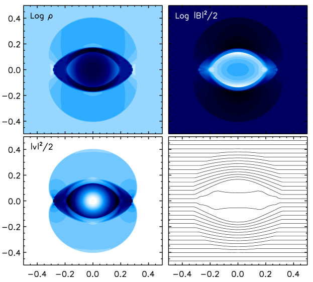
Figure 8: Colored contours for the blast wave problem at $t=0.09$. Density logarithm (upper left panel), magnetic pressure logarithm (upper right), specific kinetic energy (bottom left) and magnetic field lines (bottom right) are shown.

A uniform medium with constant density $\rho=1$ and magnetic field $\mathbf{B}=10/\sqrt{4\pi}\hat{\mathbf{i}}$ fills the square domain $[-\frac{1}{2},\frac{1}{2}]^{2}$. An over-pressurized region ($p=100$) is delimited by a small circle of radius $0.05$ centered around the origin. The speed of sound is set to unity everywhere and free-flow boundary conditions are imposed on every side of the domain.

Cylindrical explosions in Cartesian coordinates provide a useful benchmark particularly convenient in checking the robustness of the code and the response of the algorithm to different kinds of degeneracies. Fig. 8 shows the results obtained on $401^{2}$ uniform zones at $t=0.09$. The ratio of thermal and magnetic pressure is $\approx 0.251$ thus making the explosion anisotropic. The outer region is delimited by an almost cylindrical fast forward shock reaching its maximum strength on the $y$ axis (where the magnetic field is tangential) and progressively weakening as $y\to 0$. In the central region, density and magnetic fields are gradually depleted by a cylindrical rarefaction wave enclosed by an eye-shaped reverse fast shock bounding the inner edge of a higher density ring. The outer edge of this ring marks another discontinuity which degenerates into a tangential one on the $y$ axis and into a pure gas dynamical shock at the equator ($y=0$) where $B_{y}=0$. The HLLD solver provides adequate and sharp resolution of all the discontinuities and the result favorably compares to the integrations carried out with the other Riemann solvers (not shown here) and with the results of [3].

The computational execution times for the HLL, HLLD and Roe solvers stay in the ratio $1:1.21:2.01$, thus showing that the new method is approximately $20\%$ more expensive whereas the Roe solver results in computations which are almost twice as slow.

4.4 Isothermal Orszag Tang Vortex

Figure 9: Evolution of the Orszag-Tang vortex at $t=1.5$ (top) and $t=3$ (bottom). Density and magnetic pressure are shown on the left and on the right, respectively. Note the formation of a magnetic island in the center at $t=3$.

The compressible Orszag-Tang vortex system describes a doubly periodic fluid configuration undergoing supersonic MHD turbulence in two dimensions. Although an analytical solution is not known, its simple and reproducible set of initial conditions has made it a widespread benchmark for inter-scheme comparison, see for example [16]. An isothermal version of the problem was previously considered by [3]. In his initial conditions, however, the numerical value of the sound speed was not specified. For this reason, I will consider a somewhat different initial condition with velocity and magnetic fields prescribed as

$$\mathbf{v}=a\left(-\sin y\hat{\mathbf{x}}+\sin x\hat{\mathbf{y}}\right)\,,$$ (45)

$$\mathbf{B}=B_{0}\left(-\sin y\hat{\mathbf{x}}+\sin(2x)\hat{\mathbf{y}}\right)\,.$$ (46)

The value of the speed of sound is $a=2$ and the magnetic field amplitude is $B_{0}=a\sqrt{3/5}$. The density is initialized to one all over. This configuration yields a ratio of thermal to magnetic pressure of $10/3$, as in the adiabatic case. The domain is the box $[0,2\pi]^{2}$ with periodic boundary conditions imposed on all sides. Fig. 9 shows the density and magnetic pressure distributions at $t=1.5$ and $t=3$. The initial vorticity distribution spins the fluid clockwise and density perturbations steepen into shocks around $t\approx 0.7$. Because of the imposed double periodicity, shocks re-emerge on the opposite sides of the domain and broad regions of compression are formed. The dynamics is regulated by multiple interactions of shock waves, which lead to the formation of small scale vortices and density fluctuations. The shocks continuously affect the spatial distributions of density and magnetic field. Magnetic energy is dissipated through current sheets convoyed by shocks at the center of the domain where reconnection takes place around $t\approx 1.5$, through the “Y” point. By $t=3$ the kinetic energy has been reduced by more than $50\%$ and shocks have been weakened by the repeated expansions, leaving small scale density fluctuations.

Note that a magnetic island featuring a high density spot forms at the center of the domain by $t=3$. This corresponds to a change in the magnetic field topology where an “O” point forms in the central region. It should be emphasized that the same feature is observed when the Roe solver is employed during the integration and it is also distinctly recognizable in the results of [3]. However, it requires at least twice the resolution to be seen if the fluxes are computed with the HLL solver. Yet, the magnetic island does not form at sufficiently lower resolution for any solver. Although its origin has to do with the complex phenomenology of MHD reconnection which lies outside the scope of this paper, it is speculated that its presence may be numerically induced by a decreased effective resistivity across the central current sheet. Future studies should specifically investigate on this issue.

The total execution times for the three solvers (HLL, HLLD and Roe) scale as $1:1.25:2.06$, thus confirming the results obtained for the previous test problem.

5 Conclusions

A new Riemann solver for the equations of magnetohydrodynamics with an isothermal equation of state has been derived. The solver leans on a multi-state Harten-Lav-van Leer representation of the solution inside the Riemann fan, where only fast and rotational discontinuities are considered. Under this approximation, density, normal momentum and the corresponding flux components inside the solution are given by their HLL averages. This is equivalent to the assumption that normal velocity, density and total pressure may be regarded constant across the solution. It has been shown that this consistently leads to a three-state representation where only tangential vectors may be discontinuous across the inner rotational waves. The solver is simple to implement and does not require a characteristic decomposition of the Jacobian matrix.

The performances and efficiency of the new method have been demonstrated through one dimensional shock tube problems as well as multidimensional problems. In terms of accuracy, the proposed method of solution greatly improves over the traditional single-state HLL approach in that it provides adequate and superior resolution of rotational discontinuities and a reduced numerical diffusion. Furthermore, it has been found that the new “HLLD” solver yields accuracies comparable to or even better than the Roe solver by retaining simplicity and greater ease of implementation over the latter. In terms of efficiency, the proposed HLLD solver is only $\approx 20-25\%$ slower than the HLL method but considerably faster (up to $\approx 60\%$ in some cases) than the Roe scheme.

The author whishes to thank the support and hospitality received at the center of magnetic self-organization at the University of Chicago.

References

- [1] Balsara
- [2] D. S. Balsara, Linearized formulation of the Riemann problem for adiabatic and isothermal magnetohydrodynamics, Astrophysical J. Supp. 116 (1998) 119.
- [3] D. S. Balsara, Total Variation Diminishing scheme for adiabatic and isothermal magnetohydrodynamics, Astrophysical J. Supp. 116 (1998) 133.
- [4] D. S. Balsara, D.S. Spicer, A staggered mesh algorithm using high-order Godunov fluxes to ensure solenoidal magnetic fields in magnetohydrodynamic simulations, J. Comput. Phys. 149 (1999) 270.
- [5] P. Cargo, G. Gallice, Roe Matrices for Ideal MHD and Systematic Construction of Roe Matrices for Systems of Conservation Laws, J. Comput. Phys. 136 (1997) 446. DW
- [6] W. Dai, P.R. Woodward, Extension of the piecewise parabolic method to multidimensional ideal magnetohydrodynamics, J. Comput. Phys. 115 (1994) 485.
- [7] W. Dai, P.R. Woodward, An approximate Riemann solver for ideal magnetohydrodynamics, J. Comput. Phys. 111 (1994) 354.
- [8] S.F. Davis, Simplified second-order Godunov-type methods, SIAM J. Sci. Statist. Comput. 9 (1988) 445.
- [9] B. Einfeldt, C.D. Munz, P.L. Roe, B. Sjögreen, On Godunov-type methods near low densities, J. Comput. Phys 92 (1991) 273.
- [10] S. Gottlieb, C.W. Shu, Total variation diminishing Runge-Kutta schemes, Math. Comp. 67 (1998) 73-85.
- [11] A. Harten, P.D. Lax, B. van Leer, On upstream differencing and Godunov-type schemes for hyperbolic conservation laws, SIAM Rev. 25 (1983) 35.
- [12] T. Miyoshi, K. Kusano, K., A multi-state HLL approximate Riemann solver for ideal magnetohydrodynamics, J. Comp. Phys. 208 (2005) 315.
- [13] J. Kim, D. Ryu, T.W. Jones, S.S Hong, A multidimensional code for isothermal magnetohydrodynamic flows in astrophysics, Astrophysical J. 514 (1999) 506.
- [14] D. Ryu, T.W. Jones, Numerical magnetohydrodynamics in astrophysics: algorithm and tests for one-dimensional flow, Astrophysical J. 442 (1995) 228.
- [15] D. Ryu, T.W. Jones, A. Frank, Astrophysical J. 452 (1995) 785.
- [16] G. Tóth, The constraint in shock-capturing magnetohydrodynamics codes, J. Comput. Phys. 161 (2000) 605.
- [17] B. Van Leer, Towards the ultimate conservative difference scheme. II. Monotonicity and conservation combined in a second-order scheme, J. Comput. Phys. 14 (1974) 361