COMPARISON OF LARGE-SCALE FLOWS ON THE SUN MEASURED BY TIME-DISTANCE HELIOSEISMOLOGY AND LOCAL CORRELATION TRACKING TECHNIQUE

Abstract

We present a direct comparison between two different techniques time-distance helioseismology and a local correlation tracking method for measuring mass flows in the solar photosphere and in a near-surface layer: We applied both methods to the same dataset (MDI high-cadence Dopplergrams covering almost the entire Carrington rotation 1974) and compared the results. We found that after necessary corrections, the vector flow fields obtained by these techniques are very similar. The median difference between directions of corresponding vectors is 24 ^∘, and the correlation coefficients of the results for mean zonal and meridional flows are 0.98 and 0.88 respectively. The largest discrepancies are found in areas of small velocities where the inaccuracies of the computed vectors play a significant role. The good agreement of these two methods increases confidence in the reliability of large-scale synoptic maps obtained by them.

1 Motivation

There are several methods for measuring flows in surface layers of the Sun. Local helioseismology uses information about solar oscillations – frequency shifts and travel time variations – to infer the structure of solar interior and to determine flow patterns just below the surface (e.g. Zhao and Kosovichev, 2004). The local correlation tracking method measures apparent motion of specific structures to determine the flow field (e.g. motions of granules – Sobotka et al., 1999, or magnetic elements – Meunier, 2005). A similar method is feature tracking, which evaluates motions of well defined isolated features. Direct Doppler measurements provide in general just the line-of-sight component of the velocity vector, but when applied to large datasets, these can provide statistically robust information about properties of the surface flows (e.g. the discovery of supergranulation by Hart, 1956 or Leighton, Noyes, and Simon, 1962).

However, the results obtained by different methods may have discrepancies. These can be caused by the nature of the methods, e.g. due to different types of averaging, and also because of the use of different datasets from different instruments. In addition, various disturbing effects may be important. Therefore, we decided to compare the results obtained by two different methods, time-distance helioseismology and local correlation tracking (LCT), using the same set of data: high-cadence Dopplergrams, covering almost one Carrington rotation, obtained from Michelson Doppler Imager (MDI, Scherrer et al., 1995).

Solar acoustic waves ($p$ modes) are excited in the upper convection zone and travel between various points on the surface through the interior. The travel time of acoustic waves is affected by variations of the speed of sound along the propagation paths and also by mass flows. Time-distance helioseismology measurements Duvall et al. (1993) and inversions (Kosovichev, 1996, Zhao, Kosovichev, Duvall, 2001) provide a tool to study three-dimensional flow fields in the upper part of the solar convection zone with relatively high spatial resolution.

The local correlation tracking (LCT) method was originally designed for removing seeing-induced distortions in sequences of solar images November (1986), and later used for mapping motions of granules in series of white-light images of the photosphere November and Simon (1988). This method works on the principle of best match: local displacements in the image frames are determined for each position by cross-correlating pairs of sub-frames within a pre-defined spatial window (correlation window), and then the corresponding velocities are calculated from these displacements.

In some studies it has been shown that LCT technique underestimates the real velocities due to the smoothing of processed data by the correlation window. For example, in the study by Švanda, Klvaňa, and Sobotka (2006) based on synthetic Dopplergrams, it was found that the LCT code used also in this study underrepresents the magnitudes of velocities by a factor of 1.13. In Georgobiani et al. (2007), the correction factor with the same meaning was found to be 1.5. However, Georgobiani’s study was done using a another LCT code applied to simulated data and the results were compared with time-distance method applied to $f$ modes. This means that the correction factor is different for different parameters used in the LCT method and, therefore, it should be determined (calibrated) empirically for each particular study. Application of LCT to MDI Dopplergrams by DeRosa and Toomre (2004) showed the underestimation by more than 30%. Other studies also find the underrepresenting of magnitudes by LCT (Sobotka et al., 1999 – 20 %, Roudier et al., 1999 – 25 %).

Both methods provide surface or near-surface velocity vector fields. However, the results of these methods can be interpreted differently. While local helioseismology measures intrinsic plasma motions (through advection of acoustic waves), LCT measures apparent motions of structures (granules or magnetic elements). It is known that some structures do not necessarily follow the flows of the plasma on the surface. Fox example, supergranulation appears to rotate faster than the plasma (Beck and Schou, 2000), which may be caused by travelling waves (Gizon, Duvall, and Schou, 2003) or may be explained also as a projection effect (Hathaway, Williams, and Cuntz, 2006). Some older studies (e.g. Rhodes et al., 1991) also suggest that the difference in flow properties measured on the basis of structures’ motions and plasma motions is caused by a deeper anchor depth of these structures. An evolution of the pattern may also play a significant role (e.g. due to emergence of magnetic elements). Another possiblity is that surface structures are not coherent features, but patterns traveling with a different group velocity than the surface plasma velocity, such as occurs for the features present in simulations of travelling-wave convection (e.g., Hurlburt, Matthews, and Proctor, 1996).

Some attempts to compare the results of local helioseismology and the LCT method for large scales, with characteristic size 100 Mm and more, have been carried out by Ambrož (2005), but his results were inconclusive. The correlation coefficient describing the match of the velocity maps obtained by local helioseismology and the LCT method was close to zero. Nevertheless, there were compact and continuous regions of characteristic size from 30 to 60 heliographic degrees with a good agreement between the two methods, so that one could not conclude that the results were completely different. In his study, many factors could be significant: the techniques were applied to different types of datasets (LCT was applied to low resolution magnetograms acquired at the Wilcox Solar Observatory and the time-distance method used MDI Dopplergrams). Both techniques had very different spatial resolution, and also the accuracy of the measurements was not well known.

We decided to avoid these problems and analyze the same data set from the MDI instrument on SOHO. MDI provides approximately two months of continuous high-cadence (one-minute cadence) full-disc Dopplergrams each year. This Dynamics Program provides data suitable for helioseismic studies, and also for the local correlation tracking of supergranules. Thus, this is a perfect opportunity to compare the performance and results of two different techniques using the same set of data, and to avoid effects of observations with different instruments or in different conditions.

2 Data preparation

The selected dataset consists of 27 data-cubes from March 12, 2001, 0:00 UT to April 6, 2001, 0:31 UT, where each third day was used, and in these days three 8.5-hour long data-cubes were processed (so that every third day in the described interval was fully covered by measurements). Each data-cube is composed of 512 Dopplergrams with spatial resolution of 1.98${}^{\prime\prime}\,\rm px^{-1}$ at a one-minute cadence. All of the frames of each data-cube were tracked with rigid rate of 2.871 $\mu$rad s^-1, remapped with Postel’s projection with a resolution of 0.12 ^∘ px^-1 (1 500 km px^-1 at the center of the disc), and only a central meridian region was selected for further processing (with size of 256$\times$924 px covering $30\,^{\circ}$ in longitude and running from $-54\,^{\circ}$ to $+54\,^{\circ}$ in latitude), so that effects of distortions due to the projection do not play a significant role.

Tracked data-cubes were used to perform the time-distance analysis. From all the frames in each data-cube, the mean Dopplergram (like Figure 4 left) was subtracted to suppress the influence of velocity structures like supergranulation and to highlight the signals of $p$ modes. $P$ modes have their origin in the solar convection zone and travel through the solar interior to the surface. The travel-time of the wave depends on the speed of sound and on the velocity of the mass flow in the layers of the solar interior, through which the bulk is travelling. In the time-distance technique, the travel times of waves from the point in the photosphere (central point) to a surrounding annuli around this point are measured. The radius of each annulus selects wavemodes that propagate down to a specific depth, before being refracted upward toward the photosphere. Travel times are measured by the cross-correlation between Doppler velocities in the central point and velocities in the selected annuli around this point.

The mass flow velocities in the interior are calculated from the differences of travel times from the central point to the surrounding annuli and the travel times from the surrounding annuli to the central point when the state properties in the affected layers of the solar interior are known. In this study, the theoretical ray approximation is derived from the solar model S (Christensen-Dalsgaard et al., 1996). Dividing the annuli into sectors, the underlying flow field of selected orientations can be infered. For details see Kosovichev (1996), Zhao, Kosovichev, Duvall (2001), or Zhao and Kosovichev (2004).

During the process, the surface gravity wave ($f$ mode) is filtered out from the $k$–$\omega$ diagram before computing the travel times, because it has different dispersion characteristics than the $p$ modes used in this study. $F$ modes, if not filtered out, will disturb $p$ modes measurements, and it is also not straightforward to perfrom inversions if not separating two different modes. The $p$ mode inversions are less sensitive to the surface flows than $f$ mode data, but still recover the large-scale flows well.

The time-distance inversion results were smoothed by a Gaussian with FWHM of 30 px to match the resolution to the LCT method, and only the horizontal components ($v_{x}$, $v_{y}$) of the full velocity vector were used.

While for the time-distance method the $p$ modes of solar oscillations play a crucial role, they significantly influence the performance of the LCT method in a negative way. The oscillations are clearly visible in the Dopplergrams, causing random errors in the calculation of displacements. Therefore, before applying the LCT method, the oscillation signals must be suppressed. For our high-cadence data it is possible to do this using temporal averaging. According to Hathaway (1988) or more recently Hathaway et al. (2000) it is better to use a Gaussian type of temporal averaging than the boxcar one. We average the Dopplergrams over a 31-minute period with weights given by the formula

$$w(\Delta t)=\exp\left[{\frac{(\Delta t)^{2}}{2a^{2}}}\right]-\exp\left[{\frac{b^{2}}{2a^{2}}}\right]\left(1+\frac{b^{2}-(\Delta t)^{2}}{2a^{2}}\right),$$ (1)

where $\Delta t$ is the time between a given frame and the central one (in minutes), $b=16$ minutes and $a=8$ minutes. We verified that this filter suppresses the solar oscillations in the 2 – 4 mHz frequency band by a factor of more than five hundred.

The other issue significantly influencing the performance of the LCT method is the change of contrast and background intensity caused by solar rotation. Due to tracking the Doppler images with rotation, the magnitude of the line-of-sight component of the solar rotational velocity changes from frame to frame and affects the LCT results. The method interprets these changes as a motion towards the East, mainly in the central part of the solar disc, where the contrast in the structures of Dopplergrams is very low (see Figure 4 left). We suppress the influence of the moving background by subtraction of a third-order polynomial surface fit. We have tested that this provides almost the same results as the other possible procedures: local removal of the mean values and unsharp masking. Subtraction of the polynomial fit is not so sensitive to anomalies in the Dopplergrams, caused by regions with strong magnetic field.

The LCT method used in this study is described by the following parameters: the time-lag between correlated frames is 120 frames (two hours), the correlation window has a Gaussian shape with FWHM of 30 px, the correlation is measured by the sum of absolute differences of subframes (it is faster than calculation of the correlation coefficient and provides the same results), the extremum position is calculated using the nine-point method Darvann (1991). For each data-cube, the results of all the correlated pairs are averaged, so that the method provides an averaged flow field over 8.5 hours in the same sense as the time-distance analysis.

3 Results

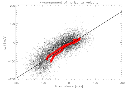
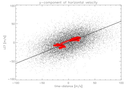
Figure 1: Left – $v_{x,{~{}\rm LCT}}$ versus $v_{x,{~{}\rm t-d}}$ plot. Red crosses denote mean zonal velocities (differential rotation) which have been used for fitting of the calibration Equation (2). Right – the same for $v_{y}$ component, the regression fit is described by Equation (3).

3.1 Statistical processing

The results containing 27 horizontal flow fields were statistically processed to obtain the cross-calibration curves for these methods. It is generally known (see discussion in Section 1, page 1) that the LCT method slightly underestimates the velocities; thus, the results should be corrected by a certain factor. From the comparison of the $x$-component of velocity (cf. Figure 1 left) we obtained parameters of a linear fit given by (numbers in parentheses denote a $\sigma$-error of the regression coefficient)

$$v_{x,{~{}\rm LCT}}=0.895(0.008)v_{x,{~{}\rm t-d}}-12.6(0.3)~{}{\rm m\,s^{-1}}.$$ (2)

The correlation coefficient between $v_{x,{~{}\rm LCT}}$ and $v_{x,{~{}\rm t-d}}$ is $\rho=0.80$. We assume that the time-distance measurements for $v_{x,{~{}\rm t-d}}$ are correct and the magnitude of the LCT measurements, $v_{x,{~{}\rm LCT}}$, must be corrected according to the slope of Equation (2). This correction factor has a value of 1.12, which is in perfect agreement with the correction factor of 1.13 found in the tests of the same LCT code using synthetic Dopplergrams with the same resolution and similar LCT parameters Švanda, Klvaňa, and Sobotka (2006). We assume that both velocity components obtained with the LCT method should be corrected by this factor.

The regression line of $v_{y}$ component (Figure 1 right) is

$$v_{y,{~{}\rm LCT}}=0.56(0.01)v_{y,{~{}\rm t-d}}+0.4(0.2)~{}{\rm m\,s^{-1}}.$$ (3)

After the slope correction using the $v_{x}$ fits, the regression curve is slightly different:

$$v_{y,{~{}\rm LCT}}=0.63(0.01)v_{y,{~{}\rm t-d}}+0.4(0.2)~{}{\rm m\,s^{-1}},$$ (4)

with the correlation coefficient between $v_{y,{~{}\rm LCT}}$ and $v_{y,{~{}\rm t-d}}$ close to 0.47. The slope of the linear fit differs significantly from the expected value 1.0.

We have tested that this asymmetry is not related to the LCT technique. The tests did not show any preference in direction of flows measured by LCT or any dependence of the results on the size of the field of view (which is not a square). Also in the recent study by Švanda, Klvaňa, and Sobotka (2006), based on synthetic data, the asymmetry between the zonal and the meridional components was not encountered.

It is possible that a drift of the supergranular pattern towards the equator (such as found by Gizon, Duvall, and Schou, 2003) might cause an asymmetry between measurements of the north-south and east-west velocities. However, this process does not explain why the meridional velocities from both techniques seem to be proportional to each other. A systematic drift would rather be depicted as a constant, or a shift depending on the latitude. However, the meridional components of velocities are generally rather small, so the errors of the measurements can play a significant role and the proportional behavior can be only apparent. Such an effect is not seen in the experiments with test data, so we do not favor this explanation.

A second explanation is based on unspecified asymmetries influencing travel-time measurements, for instance, due to different sensitivity of the MDI instrument to $p$ modes propagating in the East – West and North – South directions. Georgobiani et al. (2007) did not find such an asymmetry using $f$-mode time-distance and LCT applied to realistic numerical simulation. The asymmetry in the East – West and North – South directions observed by $p$ mode time-distance helioseismology was on the contrary noticed in a recent study based on numerically simulated data (Zhao et al., 2007). This evidence suggests the asymmetry arises only in $p$ mode inversions such as those studied here, and should be investigated further in more detail.

In this study we decided to correct the $y$-component of the time-distance results.

Figure 2: Histogram of the angular differences ($\Delta\varphi$) between directions of the velocity vectors obtained by the time-distance and LCT techniques. Dashed vertical line denotes the mean value and solid vertical line represents the median of $\Delta\varphi$.

The final calibration formulae providing the best statistical agreement between the velocities calculated using both methods are:

$$v_{x,\rm LCT,corr} = 1.12\,v_{x,\rm LCT,calc}$$ (5)

$$v_{y,\rm LCT,corr} = 1.12\,v_{y,\rm LCT,calc}$$ (6)

$$v_{x,\rm t-d,corr} = v_{x,\rm t-d,calc}$$ (7)

$$v_{y,\rm t-d,corr} = 0.63\,v_{y,\rm t-d,calc},$$ (8)

where the index corr denotes the corrected value, and the index calc denotes the original calculated value.

After the corrections, as presented in the histogram in Figure 2, the differences between the directions of the velocity vectors ($\Delta\varphi$) calculated by these techniques are quite reasonable. The mean value of the distribution is 43.56 ^∘, however, the mean value is not a good indicator in this case because the distribution function is not normal. The median value is 24.02 ^∘ and 66.6 % of points have the difference in the corresponding vector directions less than 45 ^∘.

Instead of computation of the correlation coefficient of the arguments of both vector fields, we decided to compute a magnitude-weighted cosine of $\Delta\varphi$, because it provides more robust results. This quantity is given by

$$\rho_{\rm W}=\frac{\sum|{\mathbf{v}}_{t-d}|\frac{|{\mathbf{v}}_{t-d}\cdot{\mathbf{v}}_{LCT}|}{|{\mathbf{v}}_{t-d}||{\mathbf{v}}_{LCT}|}}{\sum|{\mathbf{v}}_{t-d}|},$$ (9)

where ${\mathbf{v}}_{t-d}$ is the time-distance vector field, ${\mathbf{v}}_{LCT}$ is the LCT vector field and the summation is performed over all vectors in the field. The closer this quantity is to one, the better is the agreement between both vector fields. Larger vectors are weighted more than smaller ones. We have found that in our case $\rho_{\rm W}=0.86$.

3.2 Mean velocities

Figure 3: Left: Mean zonal velocity (thick curve) as a function of latitude (differential rotation) obtained from the time-distance data and mean zonal velocity (thin curve) obtained from the LCT data. Dashed line represents a standard rotation profile (“Snodgrass rate”). The mean zonal velocities are plotted in the coordinate system rotating rigidly with 2.871 $\mu$rad s^-1. Right: Velocities of the mean meridional flow as a function of latitude obtained by the time-distance technique (thick curve) and by the LCT method (thin curve). The correlation coefficient for the mean zonal flow is $\rho=0.98$ and for the mean meridional flow $\rho=0.88$.

 

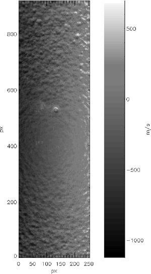
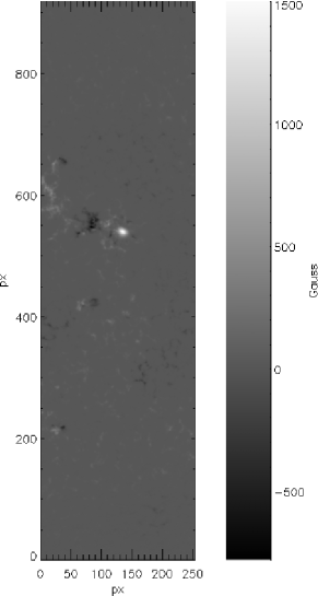
Figure 4: Part of the solar disc chosen for the detailed comparison of the results of time-distance and LCT methods. The 8.5-hour measurements are centered at March 24 2001, 4.16 UT. One pixel represents 0.12 ^∘ in heliographic coordinates. Left – Averaged MDI Dopplergram. Note the low contrast of the supergranular cells in the center of the image. This is the “blind spot” caused by prevailing horizontal motions in the photosphere. Right – Averaged MDI magnetogram.

In addition to the detailed comparison of the vector fields, we compare the mean flows, the differential rotation, and the meridional circulation. These flows can be quite simply calculated from the results of both techniques. In both cases, they provide the mean zonal and mean meridional flows for Carrington rotation 1974. The results are displayed in Figure 3, where the differential rotation curves are compared with a standard profile from Snodgrass and Ulrich (1990) in the left panel. It can be clearly seen that the latitudinal profiles for both techniques are very similar and also that the mean velocities do not differ much in magnitude. The correlation coefficients are $\rho=0.98$ for the zonal flow and $\rho=0.88$ for the meridional flow. In the differential rotation curves, the LCT results give a little slower rotation, which is also seen from Equation (2). The mean difference of average zonal velocities obtained by both techniques is 14.1 m s^-1.

We conclude that for the mean flows the results obtained by the techniques agree very well.

3.3 Detailed comparison

Figure 5: Left – Velocity field obtained by the LCT method. Right – Velocity field obtained by the time-distance technique. Both plots are centered at heliographic coordinates $b_{0}=0.0\,^{\circ}$, $l_{0}=214.3\,^{\circ}$. Units on both axes are pixels in the data frame with resolution of 0.12 ^∘ px^-1 in the Postel projection.

For a detailed comparison of the flow fields, we selected one data cube, representing 8.5-hour measurements centered at 4:16 UT March 24, 2001, $l_{0}$=214.3 ^∘ (see the averaged MDI Dopplergram and magnetogram in Figure 4). In this map, the correlation coefficient for the $x$-component of the velocity is $\rho=0.82$, for the $y$-component $\rho=0.58$, and for the vector magnitude: $\rho=0.73$. The vector plots of the flow fields obtained by both techniques, shown in Figure 5, in general seem to be quite similar to each other. However, many differences can be seen. The regions where the differences are most significant correspond to relatively small (under 50 m s^-1) velocities. This is clear from the map of the differences between the vector directions, displayed in Figure 6.

Figure 6: Difference of phases of corresponding vectors ($\Delta\varphi$). Left – for the full vector data, right – for the data with mean zonal flow substracted. In the second case the magnitudes of vectors everywhere in the studied area are comparable and the inaccuracies of individual measurements equally important. With the mean zonal flow removed the distribution of $\Delta\varphi$ become more uniform in the studied area.

The histogram of the differences between the directions of the corresponding vectors ($\Delta\varphi$) is presented in Figure 2. Values of $\Delta\varphi$ slightly anti-correlate with the average magnitude of the corresponding vectors ($\rho=-0.58$). We think that this is due to uncertainties of both techniques. From our tests using synthetic data, it became clear that the inaccuracy of the LCT code is 15 m s^-1 for velocities smaller than 100 m s^-1 and 25 m s^-1 for velocities larger than 100 m s^-1, for both components Švanda, Klvaňa, and Sobotka (2006). We think that the 10 % accuracy for the time-distance velocity vectors is a reasonable estimate. As is stated in Zhao, Kosovichev, Duvall (2001), cross-talk effects between horizontal and vertical components of flow velocities affect the time-distance inversion results. The cross-talk effect prevents us from inverting the vertical velocity correctly, but it does not block the determination of horizontal velocities (Zhao and Kosovichev, 2003). However, the vertical velocities are not discussed in this paper because they are not measured by the LCT technique. Obviously, inaccuracy in one component may cause a significant change of the direction of the horizontal vector for small velocities and, hence, the agreement of both techniques in such areas is not as good as in the areas of high velocities.

The vector velocity field may be also influenced by the temporal evolution of the traced pattern. We have tested using the full-disc MDI dopplergrams that temporal changes at mesogranular and smaller scales are effectively filtered out by a $k$–$\omega$ filter. The temporal evolution of the supergranular pattern may, in the worse case, significantly influence the calculated vector velocity field in the close (roughly equal to the FWHM of the chosen correlation window) vicinity of a rapidly changing (e.g. disappearing) supergranule.

4 Conclusions

Flow velocity fields on the solar surface obtained by two different techniques, time-distance helioseismology and local correlation tracking (LCT), were compared. Despite the fact that the first technique uses $p$ modes of solar oscillations to compute the velocity field (in the data, large-scale structures like supergranulation are suppressed), while the other one uses large-scale supergranulation pattern from averaged Doppler images as tracers for the velocity vectors determination (and requires $p$ modes removal), we found that both results match reasonably well. We have confirmed some recent studies that the LCT method slightly underestimates the actual velocities (as the consequence of a smoothing procedure), and determined empirical correction factors. After the corrections, the match in global velocity structures, mean zonal and meridional flows, is very good. The results of a detailed comparison of the vector velocity fields are not so satisfactory. However, the correlation coefficient for individual components of the flows is positive and significant, so we conclude that a meaningful match is found. It is shown that the largest disagreement is caused by very small velocities in some regions, where the errors of both methods become quite significant.