GRB 060418 and 060607A: the medium surrounding the progenitor and the weak reverse shock emission

Abstract

We constrain the circum-burst medium profile with the rise behavior of the very early afterglow light curves of gamma-ray bursts (GRBs). Using this method, we find a constant and low-density medium profile for GRB 060418 and GRB 060607A, which is consistent with the inference from the late afterglow data. In addition, we show that the absence of the IR flashes in these two afterglows is consistent with the standard hydrodynamical external reverse shock model. Although a highly magnetized model can interpret the data, it is no longer demanded. A weak reverse shock in the standard hydrodynamical model is achievable if the typical synchrotron frequency is already below the band at the shock crossing time.

1 Introduction

Quite recently, Molinari et al. (2007) reported the high-quality very early IR afterglow data of GRB 060418 and GRB 060607A. The IR afterglow lightcurves are characterized by a sharp rise ($\sim t^{3}$) and then a normal decline ($\sim t^{-1.3}$), though the simultaneous X-ray lightcurves are highly variable. The smooth joint before and after the peak time in the IR band strongly suggests a very weak reverse shock emission.

An interesting usage of these high-quality early afterglow data is to estimate the initial bulk Lorentz factor $\Gamma_{\rm o}$ of the outflow (Molinari et al. 2007). Such an estimate, of course, is dependent of the circumburst medium model [Blandford & McKee 1976, Dai & Lu 1998]. For GRB 060418, a wind profile has been ruled out by the late-time X-ray and IR afterglow data (Molinari et al. 2007). While for GRB 060607A, the X-ray data are so peculiar that the medium profile can not be reliably determined. In this work, we use the rise behavior of the very early IR data to pin down the density profile. This new method is valid for both bursts. We show that a constant and low-density medium model is favored. As a result, we confirm that Molinari et al.’s estimation of $\Gamma_{\rm o}$ for GRB 0606418 and GRB 060607A is robust.

The absence of the IR flashes for both bursts are also very interesting. Several possible solutions for non-detection of bright optical flashes in GRB afterglows have been discussed by Roming et al. (2006). To account for this failing detection, it is widely considered that the reverse shock emission would be very weak if the outflow is highly magnetized [Kennel & Coronitti 1984]. As shown in the numerical calculation of Fan, Wei & Wang (2004; Fig 1 therein), for the magnetized reverse shock, its peak optical/IR emission increases with $\sigma$ for $\sigma\leq 0.1$, then decreases for larger $\sigma$, where $\sigma$ refers to the ratio of the magnetic energy density to the particle energy density of the GRB outflow. In Fan et al. (2004), $\sigma\leq 1$ is assumed. For highly magnetized outflow (i.e., $\sigma>1$), the reverse shock emission would be suppressed further since the total electrons involved in the emission is proportional to $1/(1+\sigma)$. Zhang & Kobayashi (2005) carried out such a calculation ($\sigma\leq 100$) and got very weak reverse shock emission. In principle, the non-detection of the optical flashes could be interpreted if $\sigma\sim 100$. This conclusion motivated Molinari et al. (2007) to suggest these two GRB outflows might be magnetized. However, in this work we show that for these two bursts, the absence of the IR flashes is consistent with the standard hydrodynamical external reverse shock model [Sari & Piran 1999b, Mészáros & Rees 1999, Kobayashi 2000]. Although a highly magnetized model can interpret the data, it is no longer demanded. A weak reverse shock in the standard hydrodynamical model is achievable if the typical synchrotron frequency is already below the band at the shock crossing time.

2 Very early afterglow: constraint on the medium profile

In this section we discuss the forward shock emission because the data show no evidence for a dominant reverse shock component.

Firstly, we discuss a constant and low-density medium model. For $t<t_{\times}$, the fireball has not been decelerated significantly by the medium, where $t_{\times}$ is the time when the reverse shock crosses the outflow. The bulk Lorentz factor $\Gamma$ is thus nearly a constant, so is the typical synchrotron frequency $\nu_{m}$ [Sari et al. 1998]. On the other hand, the maximal specific flux $F_{\rm\nu,max}\propto N_{\rm e}\propto t^{3}$, where $N_{\rm e}$ is the total number of the electrons swept by the forward shock. We thus have

$$F_{\rm obs}\propto F_{\rm\nu,max}(\nu_{\rm obs}/\nu_{m})^{-(p-1)/2}\propto t^{3},$$ (1)

for $\nu_{m}<\nu_{\rm obs}<\nu_{c}$, where $\nu_{c}$ is the cooling frequency and $\nu_{\rm obs}$ is the observer’s frequency. This temporal behavior is perfectly consistent with the current data.

Secondly, we discuss a wind medium with a density profile $n_{\rm w}=3.0\times 10^{35}~{}{\rm cm^{-3}}~{}A_{*}R^{-2}$, where $R$ is the radius of the shock front to the central engine, $A_{*}=[\dot{M}/10^{-5}M_{\odot}~{}{\rm yr^{-1}}][v_{w}/(10^{8}{\rm cm}~{}{\rm s^{-1}})]$, $\dot{M}$ is the mass loss rate of the progenitor, $v_{w}$ is the velocity of the stellar wind. Again, for $t<t_{\times}$, the bulk Lorentz factor of the fireball $\Gamma$ is nearly a constant [Chevalier & Li 2000]. However, in this case, $\nu_{m}^{w}\propto t^{-1}$, $\nu_{c}^{w}\propto t$ and $F_{\rm\nu,max}^{w}\propto t^{0}$, where the superscript “$w$” represents the parameter in the wind case. The increase of the forward shock emission can not be steeper than $t^{1/2}$, as long as the self-absorption effect can be ignored [Chevalier & Li 2000]. This temporal behavior, of course, is inconsistent with the data. Can the synchrotron self-absorption shape the forward shock emission significantly and then render the wind model likely? Let’s examine this possibility. In this interpretation, $\nu_{a}^{w}(t_{\rm IR,peak})\sim 2\times 10^{14}$ Hz is required, where $\nu_{a}$ is the synchrotron self-absorption frequency of the forward shock electrons, and $t_{\rm IR,peak}$ is the peak time of the IR-band emission. In the wind model, to get a $t^{-1.3}$ IR-band light curve, we need $p\sim 2$ and $\nu_{m}^{w}<\nu_{a}^{w}<\nu_{\rm obs}<\nu_{c}^{w}$. Following Chevalier & Li (2000), it is straightforward to show that $\nu_{a}^{w}\sim 5\times 10^{13}~{}{\rm Hz}~{}\epsilon_{e,-1}^{1/3}\epsilon_{\rm B,-2}^{1/3}A_{*}^{2/3}t_{d,-3}^{-1}$ and $\nu_{c}^{w}\sim 3.5\times 10^{13}~{}{\rm Hz}~{}\epsilon_{B,-2}^{-3/2}E_{\rm k,54}^{1/2}A_{*}^{-2}[(1+z)/2]^{-3/2}t_{d,-3}^{1/2}(1+Y^{w})^{-2}$, where $\epsilon_{e}$ and $\epsilon_{B}$ are the fractions of shock energy given to the electrons and magnetic field, respectively; $z$ is the redshift, $t_{d}$ is the observer’s time in units of day, and $E_{\rm k}$ is the isotropic-equivalent kinetic energy of the outflow. Here and throughout this text, the convention $Q_{x}=Q/10^{x}$ has been adopted in cgs units.

With the requirements that at $t_{\rm IR,peak}\sim 150$s, $\nu_{a}^{w}\sim 2\times 10^{14}$ Hz and $\nu_{c}^{w}>2\times 10^{14}$ Hz, we have

$$\epsilon_{e,-1}^{1/3}\epsilon_{\rm B,-2}^{1/3}A_{*}^{2/3} \sim 8,$$ (2)

$$\epsilon_{B,-2}^{-3/2}E_{\rm k,54}^{1/2}A_{*}^{-2} > 4(1+Y^{w})^{2}.$$ (3)

These two relations yield $\epsilon_{B}<2\times 10^{-5}(1+Y^{w})^{-4}E_{k,54}\epsilon_{e}^{2}$ and $A_{*}>160~{}\epsilon_{e}^{-3/2}E_{k,54}^{-1/2}(1+Y^{w})^{2}$. For such a large contrast between $\epsilon_{e}$ and $\epsilon_{B}$, $Y^{w}\gg 1$. The resulting $\epsilon_{B}$ and $A_{*}$ are too peculiar to be acceptable.

Therefore it is very likely that the medium surrounding the GRB progenitor has a low and constant number density. This conclusion is also supported by the temporal and spectral analysis of the late time X-ray and IR afterglows of GRB 060418 [Molinari et al. 2007]. Here it is worth pointing out that though the multi-wavelength afterglow modeling of many other bursts has reached a similar conclusion [Panaitescu & Kumar 2001, Zhang et al. 2006, Nousek et al. 2006, Zhang 2007, Sollerman et al. 2007], these works were only based on the late-time afterglow data and may be invalid for the early ones. This is because the density profile of the circumburst medium, in principle, could vary over radius due to the interaction between the stellar-wind and the interstellar medium. For $R<R_{c}\sim{\rm several}\times 10^{16}-10^{17}$cm, the medium may be wind-like. At larger $R$, the stalled wind material may be ISM-like [Ramirez-Ruiz et al. 2001]. Assuming that GRB 060418 has such a density profile, we can estimate $R_{c}$ as follows. Note that at $R_{c}$, the outflow has not got decelerated, which implies that $3.8\times 10^{36}A_{*}\Gamma^{2}m_{p}c^{2}<E_{k}/2$. On the other hand, at $t_{\rm IR,peak}$ a $\Gamma_{\times}\sim 200$ is likely [Molinari et al. 2007]. We thus have

$$R_{c}<2\times 10^{15}~{}{\rm cm}~{}E_{k,54}A_{*}^{-1}.$$ (4)

3 Interpreting the absence of the reverse shock emission

3.1 General relation between forward and reverse shock peak emission: the thin fireball case

In the standard fireball afterglow model, there are two shocks formed when the fireball interacts with the medium [Piran 1999], one is the ultra-relativistic forward shock emission expanding into the medium, the other is the reverse shock penetrating into the GRB outflow material. The forward shock is long-lasting while the reverse shock is short-living. At a time $t_{\times}\sim\max\{T_{90},60(1+z)E_{k,54}^{1/3}n_{0}^{-1/3}\Gamma_{\rm o,2.5}^{-8/3}\}$, the reverse shock crosses the GRB outflow, where $n$ is the number density of the medium (please note that a dense wind medium has been ruled out for these two bursts) and $\Gamma_{\rm o}$ is the initial Lorentz factor of the GRB outflow.

If the fireball is thick, $t_{\times}\sim T_{90}$. The reverse shock emission overlaps the prompt $\gamma-$rays and is not easy to be detected [Sari & Piran 1999b, Kobayashi 2000]. In this work, we focus on the thin fireball case, in which the peak of the reverse shock emission and the prompt $\gamma-$rays are separated. The relatively longer reverse shock emission renders it more easily to be recorded by the observers. In this case,

$$t_{\times}\sim 60(1+z)~{}{\rm s}~{}E_{k,54}^{1/3}n_{0}^{-1/3}\Gamma_{\rm o,2.5}^{-8/3}.$$ (5)

After that time, the dynamics of the forward shock can be well approximated by the Blandford-McKee similar solution [Blandford & McKee 1976], which emission can be estimated by

$$F_{\nu,{\rm max}}=6.6~{}{\rm mJy}~{}({1+z\over 2})D_{L,28.34}^{-2}\epsilon_{B,-2}^{1/2}E_{k,53}n_{0}^{1/2},$$ (6)

$$\nu_{m}=2.4\times 10^{16}~{}{\rm Hz}~{}E_{\rm k,53}^{1/2}\epsilon_{\rm B,-2}^{1/2}\epsilon_{e,-1}^{2}C_{p}^{2}({1+z\over 2})^{1/2}t_{d,-3}^{-3/2},$$ (7)

$$\nu_{c}=4.4\times 10^{16}~{}{\rm Hz}~{}E_{k,53}^{-1/2}\epsilon_{B,-2}^{-3/2}n_{0}^{-1}({1+z\over 2})^{-1/2}t_{d,-3}^{-1/2}{1\over(1+Y)^{2}},$$ (8)

where $p$ is the power-law index of the shocked electrons, $C_{p}\equiv 13(p-2)/[3(p-1)]$, the Compton parameter $Y\sim(-1+\sqrt{1+4\eta\epsilon_{e}/\epsilon_{B}})/2$, $\eta\sim\min\{1,(\nu_{m}/\bar{\nu}_{c})^{(p-2)/2}\}$ and $\bar{\nu}_{c}=(1+Y)^{2}\nu_{c}$.

Following Zhang et al. (2003) and Fan & Wei (2005), we assume that $\epsilon_{e}^{\rm r}={\cal R}_{\rm e}\epsilon_{\rm e}$ and $\epsilon_{\rm B}^{\rm r}={\cal R}_{\rm B}^{2}\epsilon_{\rm B}$, where the superscript “$r$” represents the parameter of the reverse shock. At $t_{\times}$, the reverse shock emission are governed by [Fan & Wei 2005]

$$\nu_{\rm m}^{\rm r}(t_{\rm\times})={\cal R}_{\rm B}[{\cal R}_{\rm e}(\gamma_{34,\times}-1)]^{2}\nu_{\rm m}(t_{\rm\times})/(\Gamma_{\times}-1)^{2},$$ (9)

$$\nu_{\rm c}^{\rm r}(t_{\times})\approx{\cal R}_{\rm B}^{-3}[(1+Y)/(1+Y^{\rm r})]^{2}\nu_{\rm c}(t_{\times}),$$ (10)

$$F_{\rm\nu,max}^{\rm r}(t_{\rm\times})\approx\Gamma_{\rm o}{\cal R}_{\rm B}F_{\rm\nu,max}(t_{\rm\times}),$$ (11)

where $\gamma_{34,\times}\approx(\Gamma_{\rm o}/\Gamma_{\times}+\Gamma_{\times}/\Gamma_{\rm o})/2$ is the Lorentz factor of the shocked ejecta relative to the initial outflow (note that we focus on the “thin fireball case”), $\Gamma_{\times}\sim\Gamma_{\rm o}/2$ is the bulk Lorentz factor of the shocked ejecta at $t_{\times}$, $Y^{\rm r}\simeq[-1+\sqrt{1+4\eta^{\rm r}{\cal R}_{\rm e}\epsilon_{\rm e}/({\cal R}_{\rm B}^{2}\epsilon_{\rm B})}]/2$ is the Compton parameter, $\eta^{\rm r}\approx{\rm min}\{1,~{}(\nu_{\rm m}^{\rm r}/\bar{\nu}_{\rm c}^{\rm r})^{\rm(p-2)/2}\}$ and $\bar{\nu}_{c}^{\rm r}=(1+Y^{\rm r})^{2}\nu_{c}^{\rm r}$.

With the observer frequency $\nu_{\rm obs}$, $\nu_{m}^{\rm r}(t_{\times})$, $\nu_{c}^{\rm r}(t_{\times})$ and $F_{\rm\nu,max}^{\rm r}(t_{\times})$, it is straightforward to estimate the peak flux of the reverse shock emission [Sari & Piran 1999a]. For the IR/optical emission (i.e., $\nu_{\rm obs}\sim 2-5\times 10^{14}$ Hz) that interests us here, we usually have $\nu_{m}^{\rm r}(t_{\times})<\nu_{\rm obs}<\nu_{c}^{\rm r}(t_{\times})$. The observed reverse shock emission is thus

$$F^{\rm r}_{\rm obs}(t_{\times}) \approx F_{\rm\nu,max}^{\rm r}(t_{\times})[\nu_{\rm obs}/\nu_{m}^{\rm r}(t_{\times})]^{-(p-1)/2}.$$ (12)

With eq.(9),(11) and the relation $\Gamma_{\times}\sim\Gamma_{\rm o}/2$, we have

$${F^{\rm r}_{\rm obs}(t_{\times})\over F_{\rm\nu,max}} \approx \Gamma_{\rm o}{\cal R}_{\rm B}^{(p+1)\over 2}[{{\cal R}_{\rm e}(\gamma_{34}(t_{\times})-1)\over\Gamma(t_{\times})-1}]^{p-1}[{\nu_{\rm obs}\over\nu_{m}(t_{\times})}]^{-(p-1)\over 2}$$ (13)

$$\approx 2^{\rm 1-p}\Gamma_{\rm o}^{\rm 2-p}{\cal R}_{\rm e}^{\rm p-1}{\cal R}_{\rm B}^{\rm p+1\over 2}[{\nu_{\rm obs}\over\nu_{m}(t_{\times})}]^{-(p-1)\over 2}$$

$$\approx 0.08{\cal R}_{\rm e}^{\rm p-1}{\cal R}_{\rm B}^{\rm p+1\over 2}[{\nu_{\rm obs}\over\nu_{m}(t_{\times})}]^{-(p-1)\over 2},$$

and

$$F^{\rm r}_{\rm obs}(t_{\times})\over F_{\rm obs}(t_{\times}) = F^{\rm r}_{\rm\nu,max}[{\nu_{\rm obs}/\nu^{\rm r}_{m}(t_{\times})}]^{-(p-1)/2}\over{F_{\rm\nu,max}[\nu_{\rm obs}/\nu_{m}(t_{\times})]^{-(p-1)/2}}$$ (14)

$$\approx \Gamma_{\rm o}{\cal R}_{\rm B}^{(p+1)\over 2}{\cal R}_{\rm e}^{p-1}(\gamma_{34,\times}-1)^{p-1}(\Gamma_{\times}-1)^{1-p}$$

$$\approx 0.08{\cal R}_{\rm e}^{p-1}{\cal R}_{\rm B}^{p+1\over 2},$$

for $\nu_{\rm m}(t_{\times})\leq\nu_{\rm obs}\leq\nu_{\rm c}(t_{\times})$, or

$$F^{\rm r}_{\rm obs}(t_{\times})\over F_{\rm obs}(t_{\times}) = F^{\rm r}_{\rm\nu,max}[{\nu_{\rm obs}/\nu^{\rm r}_{m}(t_{\times})}]^{-(p-1)/2}\over{F_{\rm\nu,max}[\nu_{\rm obs}/\nu_{m}(t_{\times})]^{1/3}}$$ (15)

$$\approx 0.08{\cal R}_{\rm e}^{p-1}{\cal R}_{\rm B}^{p+1\over 2}[{\nu_{\rm obs}\over\nu_{m}(t_{\times})}]^{-{3p-1\over 6}},$$

for $\nu_{\rm c}(t_{\times})>\nu_{\rm m}(t_{\times})>\nu_{\rm obs}$, here $p\sim 2.3$ and $\Gamma_{\rm o}\sim 200$ have been taken into account. For a $p$ closer to 2, the coefficient 0.08 in Eqs.(13-15) should be lager. Eqs.(13-15) are the main result of this paper. It is now evident that to have a ${F^{\rm r}_{\rm obs}(t_{\times})\geq F_{\rm obs}(t_{\times})}$, we need ${\cal R}_{\rm e}\gg 1$, or ${\cal R}_{\rm B}\gg 1$, or ${\nu_{\rm obs}\ll\nu_{m}(t_{\times})}$. If ${\nu_{\rm obs}\ll\nu_{m}(t_{\times})}<\nu_{c}(t_{\times})$, the forward shock will peak at a time $t_{p}$ when $\nu_{m}(t_{p})\approx(t_{p}/t_{\times})^{-3/2}\nu_{m}(t_{\times})\approx\nu_{\rm obs}$. So eq.(13) and eq.(15) can be re-written as

$${F^{\rm r}_{\rm obs}(t_{\times})\over F_{\rm\nu,max}}={F^{\rm r}_{\rm obs}(t_{\times})\over F_{\rm obs}(t_{p})}\approx 0.08{\cal R}_{\rm e}^{\rm p-1}{\cal R}_{\rm B}^{\rm p+1\over 2}({t_{p}\over t_{\times}})^{3(p-1)\over 4}.$$ (16)

$${F^{\rm r}_{\rm obs}(t_{\times})\over F_{\rm obs}(t_{\times})}\approx 0.08{\cal R}_{\rm e}^{\rm p-1}{\cal R}_{\rm B}^{\rm p+1\over 2}({t_{p}\over t_{\times}})^{3p-1\over 4}.$$ (17)

In the standard reverse shock model [Sari & Piran 1999b, Mészáros & Rees 1999, Kobayashi 2000], ${\cal R}_{\rm e}={\cal R}_{\rm B}=1$. So to have a optical flash brighter than the forward shock emission ( $F^{\rm r}_{\rm obs}(t_{\times})>F_{\rm obs}(t_{p})$ ), we need

$$\nu_{m}(t_{\times})>125^{\rm 1/(p-1)}\nu_{\rm obs}~{}~{}{\rm or}~{}~{}t_{p}>29^{1/(p-1)}t_{\times}.$$ (18)

But to have a bright optical flash to outshine the forward shock emission ( $F^{\rm r}_{\rm obs}(t_{\times})>F_{\rm obs}(t_{\times})$ ), we just need

$$\nu_{m}(t_{\times})>12.5^{\rm 6/(3p-1)}\nu_{\rm obs}~{}~{}{\rm or}~{}~{}t_{p}>5^{6/(3p-1)}t_{\times}.$$ (19)

For typical GRB forward shock parameters $\epsilon_{e,-1}\sim\epsilon_{B,-2}\sim E_{\rm k,53}\sim 1$ and $p\sim 2.3$, at $t_{\times}\sim 100$ s, we have $\nu_{m}(t_{\times})\sim 50\nu_{\rm obs}$ and $F^{\rm r}_{\rm obs}(t_{\times})\sim F_{\rm\nu,max}\sim F_{\rm obs}(t_{p})\sim 4F_{\rm obs}(t_{\times})$. This simple estimate is consistent with the results of some recent/detailed numerical calculations [Nakar & Piran 2004, McMahon et al. 2006, Yan et al. 2007].

However, it is not clear whether these parameters, derived from modelling the late afterglow data [Panaitescu & Kumar 2001], are still valid for the very early afterglow data. We need high-quality early IR/optical afterglow data to pin down this issue.

3.2 Case study

Analytical approach. For GRB 060418 and GRB 060607A, their parameters $(T_{90},~{}z,~{}E_{\gamma,52},~{}F_{\rm IR,peak},~{}t_{\rm IR,peak})$ are $(50{\rm s},~{}1.489,~{}9,~{}50{\rm mJy},~{}153{\rm s})$ and $(100{\rm s},~{}3.082,~{}10,~{}20{\rm mJy},~{}180{\rm s})$, respectively [Molinari et al. 2007]. Here $E_{\gamma}$ is the isotropic-equivalent prompt gamma-ray energy. As shown in Molinari et al. (2007), for $t>t_{\rm IR,peak}$, both the temporal and the spectral data of GRB 060418 are well consistent with a slow-cooling fireball expanding into a constant medium. To interpret the afterglow of GRB 060607A, however, is far more challenging. We note that the ratio between the X-ray flux and the IR flux increases with time sharply and the late time X-ray afterglow flux drops with time steeper than $t^{-4}$. These two peculiar features, of course, can not be interpreted normally. One speculation is that nearly all the X-ray data are the so-called “central engine afterglow” (i.e., the prompt emission of the prolonged activity of the central engine; see Katz, Piran & Sari [1998], Fan, Piran & Xu [2006]; Zhang, Liang & Zhang [2007]) and are independent of the IR afterglow [Fan & Wei 2005, Zhang et al. 2006]. This kind of ad hoc speculation is hard to be confirmed or to be ruled out. However, the similarity between these two early IR band afterglow light curves implies that both of them may be the forward shock emission of a slow-cooling fireball.

Hereafter we focus on GRB 060418. The peak H-band flux is $\sim 50$ mJy, while the peak X-ray emission attributed to the forward shock emission is likely to be $\sim 0.15$ mJy [Molinari et al. 2007]. The contrast is just $\sim 300$, which suggests a $\nu_{\rm c}(t_{\rm IR,peak})\sim 2.4\times 10^{17}$ Hz, where a $p=2.6\pm 0.1$ has been taken into account [Molinari et al. 2007]. On the other hand, in the slow cooling phase, the observed flux peaks because the observer’s frequency crosses $\nu_{m}$ or the peak time $\sim t_{\times}$ for $\nu_{m}<\nu_{\rm obs}$. So we have two more constraints: $\nu_{m}(t_{\rm IR,peak})\leq 1.8\times 10^{14}$ Hz and $F_{\rm\nu,max}\geq 50$ mJy.

With eqs.(6-8), it is straightforward to show that

$$\epsilon_{B,-2}^{1/2}E_{\rm k,53}n_{0}^{1/2}\geq 20,$$ (20)

$$\epsilon_{B,-2}^{1/2}E_{\rm k,53}^{1/2}\epsilon_{e,-1}^{2}\leq 6\times 10^{-3},$$ (21)

$$\epsilon_{B,-2}^{-3/2}E_{\rm k,53}^{-1/2}n_{0}^{-1}(1+Y)^{-2}\sim 8.$$ (22)

These relations are satisfied with $(E_{\rm k,53},~{}n_{0},~{}\epsilon_{e},~{}\epsilon_{B},~{}p)\sim(100,~{}1,~{}0.004,~{}0.001,~{}2.6)$.

Is $t_{\times}\sim t_{\rm IR,peak}$? The answer is positive. If $t_{\times}<t_{\rm IR,peak}$, the IR band flux will increase with time as $t^{3}$ for $t\leq t_{\times}$ and then change with time as $t^{1/2}$ for $t_{\times}<t<t_{\rm IR,peak}$ [Sari et al. 1998]. This is inconsistent with the observation. So we have $t_{\times}\sim t_{\rm IR,peak}>T_{90}$ and the fireball is thin. Our assumption made in the last subsection is thus valid. Now $\nu_{\rm m}(t_{\times})\approx\nu_{\rm m}(t_{\rm IR,peak})\leq\nu_{\rm obs}$. With eq.(13) and ${\cal R}_{\rm e}={\cal R}_{\rm B}=1$, we have

$${F^{\rm r}_{\rm obs}(t_{\times})\over F_{\rm obs}(t_{\times})}\sim{\cal O}(0.1).$$ (23)

So the reverse shock emission is too weak to dominate over that of the forward shock. The non-detection of the IR flashes in GRB 060418 and GRB 060607A has then been well interpreted.

Numerical fit to the afterglow of GRB 060418. The code used here to fit the multi-band lightcurves has been developed by Yan et al. (2007), in which both the reverse and the forward shock emission have been taken into account. As mentioned in the analytical investigation, the X-ray data are flare-rich. These flares, of course, are very hard to be understood in the external forward shock model. Instead it may be attributed to the prolonged activity of the central engine (Fan & Wei 2005; Zhang et al. 2006). Assuming that the power-law decaying part (i.e., excluding the flares) is the forward shock emission, the small contrast between the X-ray and the H-band flux at $t_{\rm IR,peak}$ requires a $\nu_{\rm c}\sim 2.4\times 10^{17}$ Hz and thus a small $\epsilon_{\rm B}$ and a normal $n$. The very early peak of the IR-band afterglow light curves strongly suggests an unusual small $\epsilon_{e}$. The relatively bright IR-band peak emission implies a very large $E_{\rm k}$.

Our numerical results have been presented in Fig.1. The best fit parameters are $(E_{\rm k,53},~{}n_{0},~{}\epsilon_{e},~{}\epsilon_{B},~{}p,~{}\Gamma_{0})\sim(300,~{}1,~{}0.005,~{}0.0002,~{}2.5,~{}600)$. The reverse shock emission is too weak to outshine the forward shock emission (note that in this work, ${\cal R}_{\rm e}={\cal R}_{\rm B}=1$ are assumed), as predicted before. In the calculation, we did not take into account the external Inverse Compton (EIC) cooling by the flare photons. Here we discuss it analytically. Following Fan & Piran (2006b), the EIC cooling parameter can be estimated by $Y_{\rm EIC}\sim 0.4L_{\rm flare,48.7}\epsilon_{\rm B,-3.7}^{-1}E_{\rm k,55.5}^{-1}{\Delta T}_{3}$, where $L_{\rm flare}$ is the luminosity of the flare and $\Delta T$ is the duration of the flare. Such a cooling correction is so small that can be ignored.

The half-opening angle $\theta_{j}$ of the ejecta can not be well determined with the current data. The lack of the jet break in H-band up to $t_{d}\sim 0.1$ suggests a $\theta_{j}>0.024$. So a robust estimate of the intrinsic kinetic energy of GRB 060418 is $\sim E_{\rm k}\theta_{j}^{2}/2>8\times 10^{51}$ erg.

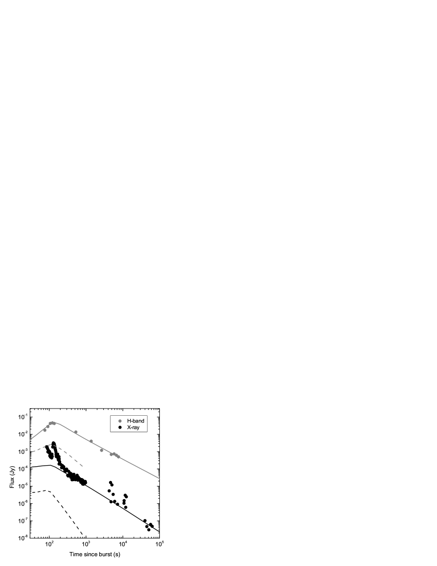
Figure 1: Numerical fit to the afterglow of GRB060418. The solid and dashed lines represent the emission from the forward and reverse shock.

4 Three kinds of reverse shock emission light curves?

Zhang et al. (2003) suggested that there could be two types of reverse shock emission light curves. Type-I is like that of GRB 041219a (Blake et al. 2005), in which both the forward and the reverse shock peak emission are present [$F^{\rm r}_{\rm obs}(t_{\times})>F_{\rm obs}(t_{\times})$ and $F^{\rm r}_{\rm obs}(t_{p})\sim F_{\rm obs}(t_{p})$]. Type-II is like that of GRB 990123 (Akerlof et al. 1999), in which the reverse shock emission component is so strong that outshines the peak emission of the forward shock, i.e., $F^{\rm r}_{\rm obs}(t_{p})\gg F_{\rm obs}(t_{p})$. The difference between these two kinds of reverse shock emission has been attributed to the very different magnetization (${\cal R}_{\rm B}$). For GRB 990123, ${\cal R}_{\rm B}\sim 20$ (Fan et al. 2002; Zhang et al. 2003); whereas for GRB 041219a, ${\cal R}_{\rm B}\sim 3$ (Fan, Zhang & Wei 2005).

GRB 060418 and GRB 060607A could be classed into Type-III, in which the reverse shock emission is absent, i.e., $F^{\rm r}_{\rm obs}(t_{\times})\ll F_{\rm obs}(t_{\times})$. We summarize these three types of early afterglow light curves in Fig.2. The possible physical causes are also presented. Fig.3 is to identify these three types in the ${\cal R}_{\rm B}-{\cal R}_{\rm t}$ plane, where $R_{\rm t}\equiv t_{\rm p}/t_{\times}$.

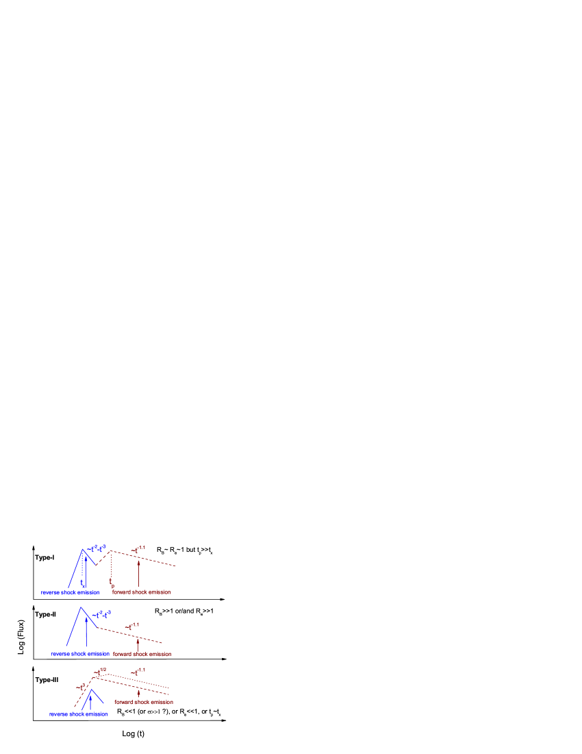
Figure 2: Three types of GRB early optical afterglows. Type-I and Type-II were defined in Zhang et al. (2003). Dashed and dotted lines in Type-III represent the forward shock emission for $\nu_{\rm m}(t_{\times})<\nu_{\rm obs}<\nu_{\rm c}(t_{\times})$ and $\nu_{\rm c}(t_{\times})>\nu_{\rm m}(t_{\times})>\nu_{\rm obs}$, respectively.

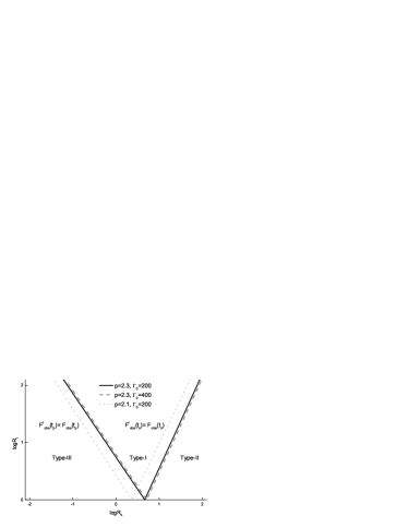
Figure 3: Assuming the observer frequency located in $\nu_{m}^{\rm r}(t_{\times})<\nu_{\rm obs}<\nu_{c}^{\rm r}(t_{\times})$ and $\nu_{\rm obs}<\nu_{m}(t_{\times})$, taking ${\cal R}_{\rm e}=1$, we identify the regimes for the three types of GRB early optical afterglow light curves.

5 The polarimetry of prompt emission or very early afterglow: constraint on the physical composition of GRB outflow

The polarimetry of prompt emission or very early afterglow (i.e., the reverse shock emission) is very important for diagnosing the composition of the GRB outflow, since the late afterglow, taking place hours after the trigger, is powered by the external forward shock, so that essentially all the initial information about the ejecta is lost.

If the GRB ejecta is highly magnetized, the prompt $\gamma-$ray/X-ray/UV/optical emission and the reverse shock emission should be linearly polarized (Lyutikov, Pariev & Blandford 2003; Granot 2003; Fan et al. 2004). This is because the magnetic fields from the central engine are likely frozen in the expanding shells. The toroidal magnetic field component decreases as $r^{-1}$, while the poloidal magnetic field component decreases as $r^{-2}$. At the typical radius for “internal” energy dissipation or the reverse shock emission, the frozen-in field is dominated by the toroidal component. For an ultra-relativistic outflow, due to the relativistic beaming effect, only the radiation from a very narrow cone (with the half-opening angle $\leq 1/\Gamma$) around the line of sight can be detected. As long as the line of sight is off the symmetric axis of the toroidal magnetic field, the orientation of the viewed magnetic field is nearly the same within the field of view. The synchrotron emission from such an ordered magnetic field therefore has a preferred polarization orientation (i.e. the direction of the toroidal field). Consequently, the linear polarization of the synchrotron emission of each electrons can not be averaged out and the net emission should be highly polarized (see Fan et al. 2005a and the references therein).

In a few events, the prompt $\gamma-$ray polarimetry are available but the results are quite uncertain. Even for the very bright GRB 041219a, a systematic effect that could mimic the weak polarisation signal could not be excluded [McGlynn et al. 2007]. So far, the most reliable polarimetry is that in UV/optical band (e.g., Gorosabel et al. 2006). The optical polarimetry of the prompt emission and the reverse shock emission requires a quick response of the telescope to the GRB alert and is thus challenging. Very recently, Mundell et al. (2007a) reported the optical polarization of the afterglow, at 203 sec after the initial burst of $\gamma-$rays from GRB 060418, using a ring polarimeter on the robotic Liverpool Telescope. The percentage of polarization is $\leq 8\%$. As shown in our section 3, the reverse shock emission of GRB 060418 is very weak. So the optical emission at 203 sec is mainly from the forward shock, for which a polarization $\leq 8\%$ is quite natural. The polarimetry of this particular burst thus does not help us too much to probe the GRB outflow composition. However, the successful polarization measurement at such an early time demonstrates the feasibility of detecting the polarization of prompt optical emission or reverse shock emission. We expect significant detections in the following cases: (a) Long GRBs followed by bright IR/optical flash, for example, GRB 990123 and GRB 041219a [Blake et al. 2005]; (b) The super-long GRBs with prompt IR/optical emission, for example, GRB 041219a [Vestrand et al. 2005]; (c) The bright optical flare simultaneous with an X-ray flare, for example, GRB 050904 [Boër et al. 2006]. The positive polarization measurement of these events is not only a reliable diagnosis of the physical composition of the GRB/X-ray flare outflow but also a good probe of the Quantum Gravity (see Fan, Wei & Xu 2007 and the references therein).

6 Summary

The temporal behavior of the very early afterglow data is valuable to constrain the medium profile surrounding the progenitor. For GRB 060418 and GRB 060607A, the sharp increase of the very early H-band afterglow light curve has ruled out a WIND-like medium. This conclusion is further supported by the late time X-ray and IR afterglow data of GRB 060418. This rather robust argument is inconsistent with the canonical collapsar model, in which a dense stellar wind medium is expected. More fruitful very early IR/optical data are needed to draw a more general conclusion.

The absence of the reverse shock signatures in the high-quality IR afterglows of GRB 060418 and GRB 060607A may indicate the outflows being strongly magnetized. We, instead, show that the non-detection of IR flashes in these two events is consistent with the standard reverse shock model. Although a highly magnetized model can interpret the data, it is no longer demanded. The physical reason is that in these two bursts, $\nu_{m}(t_{\times})\sim 2-5\times 10^{14}$ Hz. Such a small $\nu_{m}(t_{\times})$ will influence our observation in two respects. One is that $\nu^{\rm r}_{m}(t_{\times})\sim\nu_{m}(t_{\times})/4\Gamma_{\rm o}^{2}\sim 10^{9}{\rm Hz}$. The corresponding emission in IR band is thus very weak. The other is that now the forward shock peaks at IR/optical band at $t_{\times}$. Consequently, the IR/optical emission of the reverse shock can not dominate over that of the forward shock.

It is not clear whether the absence of the optical flashes in most GRB afterglows [Roming et al. 2006] can be interpreted in this way or not. Of course, one can always assume ${\cal R}_{\rm e}\ll 1$ or/and ${\cal R}_{\rm B}\ll 1$ to solve this puzzle. But before adopting these phenomenological approaches, one should explore the physical processes that could give rise to these modifications. The Poynting flux dominated outflow ($\sigma\sim 100$ after the prompt $\gamma$-ray phase) can account for the absence of the IR/optical flashes in GRB afterglows. Again, before accepting such an interpretation, we need independent probe of the physical composition of the GRB outflow. Anyway, we do find that in some bursts, for example, GRB 050319 [Mason et al. 2006], GRB 050401 [Rykoff et al. 2005], and GRB 061007 [Mundell et al. 2007b, Schady et al. 2007], the optical afterglow flux drops with time as a single power for $t>{\rm several}\times 100$ s and strongly implies a very small $\nu_{m}(t_{\times})$. It is likely that the non-detection of the IR/optical flash in some bursts are consistent with the standard reverse shock model and thus not to our surprise.

So far the physical composition of the GRB outflow is not clear, yet. If the GRB outflow is just mildly magnetized, there are two important signatures. One is that the prompt emission as well as the reverse shock emission should be highly polarized (Lyutikov, Pariev & Blandford 2003; Granot 2003; Fan et al. 2004). The other is that the reverse shock emission should be much brighter than the non-magnetization case [Fan et al. 2004, Zhang & Kobayashi 2005]. It is interesting to note that both signatures may have been detected in GRB 041219a. By modelling the reverse/forward shock emission of GRB 041219a, Fan et al. (2005b) showed that the reverse shock region was weakly magnetized. Very recently, McGlynn et al. (2007) found possible evidence for the high linear polarization of the prompt $\gamma-$rays. These findings are consistent with the mildly magnetized outflow model of GRBs. Thanks to the successful performance of the ring polarimeter on the robotic Liverpool Telescope, a reliable UV/optical polarimetry of the prompt or reverse shock emission is possible [Mundell et al. 2007a]. The nature of the outflow could thus be better constrained in the near future.

References

- [] Akerlof C., et al. 1999, Nature, 398, 400
- [Blake et al. 2005] Blake C. H., et al., 2005, Nature, 435, 181
- [Blandford & McKee 1976] Blandford R. D., McKee C. F., 1976, Phys. Fluids., 19, 1130
- [Boër et al. 2006] Boër, M., Atteia, J. L., Damerdji, Y., Gendre, B., Klotz, A., & Stratta, G. 2006, ApJ, 638, L71
- [Chevalier & Li 2000] Chevalier R. A., Li Z. Y., 2000, ApJ, 536, 195
- [Dai & Lu 1998] Dai Z. G., Lu T., 1998, MNRAS, 298, 87
- [Fan et al. 2002] Fan Y. Z., Dai Z. G., Huang Y. F., Lu T., 2002, Chin. J. Astron. Astrophys., 2, 449
- [Fan & Piran 2006a] Fan Y. Z., Piran T., 2006a, MNRAS, 369, 197
- [Fan & Piran 2006b] Fan Y. Z., Piran T., 2006b, MNRAS, 370, L24
- [Fan et al. 2006] Fan Y. Z., Piran T., Xu D., 2006, JCAP, 0609, 013
- [Fan & Wei 2005] Fan Y. Z., Wei D. M., 2005, MNRAS, 364, L42
- [Fan et al. 2004] Fan Y. Z., Wei D. M., Wang C. F., 2004, A&A, 424, 477
- [Fan et al. 2007] Fan Y. Z., Wei D. M., Xu D., 2007, MNRAS in press (astro-ph/0702006)
- [Fan, Zhang & Proga 2005a] Fan Y. Z., Zhang B., Proga D., 2005a, ApJ, 635, L129
- [Fan, Zhang & Wei 2005b] Fan Y. Z., Zhang B., Wei D. M., 2005b, ApJ, 628, L25
- [Gao & Fan 2006] Gao W. H., Fan Y. Z., 2006, Chin. J. Astron. Astrophys, 6, 513
- [Gorosabel et al. 2006] Gorosabel J., et al., 2006, A&A, 459, L33
- [Granot 2003] Granot, J. 2003, ApJ, 596, L17
- [Katz et al. 1998] Katz J. I., Piran T., Sari R., 1998, Phys. Rev. Lett., 80, 1580
- [Kennel & Coronitti 1984] Kennel C. F., & Coronitti E. V., 1984, ApJ, 283, 694
- [Kobayashi 2000] Kobayashi S., 2000, ApJ, 545, 807
- [Lyutikov et al. 2003] Lyutikov, M., Pariev, V. I., & Blandford, R. D. 2003, ApJ, 597, 998
- [Mason et al. 2006] Mason K. O., et al., 2006, ApJ, 639, 361
- [McGlynn et al. 2007] McGlynn S et al. , 2007, A&A, in press (astro-ph/0702738)
- [McMahon et al. 2006] McMahon E., Kumar P., Piran, T., 2006, MNRAS, 366, 575
- [Mészáros & Rees 1999] Mészáros, P., & Rees, M. J., 1999, MNRAS, 306, L39
- [Molinari et al. 2007] Molinari E. et al. , 2007, A&A, submitted (astro-ph/0612607)
- [Mundell et al. 2007a] Mundell C. G. et al., 2007a, Science, in press (astro-ph/0703654)
- [Mundell et al. 2007b] Mundell C. G. et al., 2007b, ApJ, in press (astro-ph/0610660)
- [Nousek et al. 2006] Nousek, J. A. et al., 2006, ApJ, 642, 389
- [Nakar & Piran 2004] Nakar E., Piran T., 2004, MNRAS, 353, 647
- [Panaitescu & Kumar 2001] Panaitescu A., Kumar P., 2001, ApJ, 560, 49
- [Piran 1999] Piran T., 1999, Phys. Rep., 314, 575
- [Ramirez-Ruiz et al. 2001] Ramirez-Ruiz E, Dray L. M., Madau P., Tout C. A., 2001, MNRAS, 327, 829
- [Roming et al. 2006] Roming, P. W. A., et al. , 2006 , ApJ, 652, 1416
- [Rykoff et al. 2005] Rykoff E. S., et al. 2005, ApJ, 631, L121
- [Sari & Piran 1999a] Sari R., Piran T., 1999a, ApJ, 517, L109
- [Sari & Piran 1999b] Sari R., Piran T., 1999b, ApJ, 520, 641
- [Sari et al. 1998] Sari R., Piran T., Narayan R., 1998, ApJ, 497, L17
- [Schady et al. 2007] Schady P., 2007, MNRAS, submittd (astro-ph/0611081)
- [Sollerman et al. 2007] Sollerman J., 2007, A&A, in press (astro-ph/0701736)
- [Troja et al. 2007] Troja E. et al. , 2007, ApJ, submitted (astro-ph/070220)
- [Vestrand et al. 2005] Vestrand W. T. et al., 2005, Nature, 435, 178
- [Wu et al. 2007] Wu X. F., Dai Z. G., Wang X. Y., Huang Y. F., Feng L. L., Lu T., 2007, ApJ, submitted (astro-ph/0512555)
- [Yan et al. 2007] Yan T., Wei D. M., Fan Y. Z., 2007, Chin. J. Astron. Astrophys., submitted (astro-ph/0512179)
- [Zhang 2007] Zhang B., 2007, Chin. J. Astron. Astrophys., 7, 1
- [Zhang et al. 2006] Zhang B., Fan Y. Z., Dyks J., Kobayashi S., Mészáros P., Burrows D. N., Nousek J. A., Gehrels N. 2006, ApJ, 642, 354
- [Zhang & Kobayashi 2005] Zhang B., Kobayashi S., 2005, ApJ, 628, 315
- [Zhang et al. 2003] Zhang B., Kobayashi S., Mészáros P., 2003, ApJ, 595, 950
- [Zhang et al. 2007] Zhang B. B., Liang E. W., & Zhang B., ApJ, submitted (astro-ph/0612246)