New limits on the density of the extragalactic background light in the optical to the far infrared from the spectra of all known TeV blazars

Abstract

Aims. The extragalactic background light (EBL) in the ultraviolet to far-infrared wavelength region carries important information about galaxy and star formation history. Direct measurements are difficult, especially in the mid infrared region. We derive limits on the EBL density from the energy spectra of distant sources of very high energetic $\gamma$-rays (VHE $\gamma$-rays).

Methods. The VHE $\gamma$-rays are attenuated by the photons of the EBL via pair production, which leaves an imprint on the measured spectra from distant sources. So far, there are 14 detected extragalactic sources of VHE $\gamma$-rays, 13 of which are TeV blazars. With physical assumptions about the intrinsic spectra of these sources, limits on the EBL can be derived. In this paper we present a new method of deriving constraints on the EBL. Here, we use only very basic assumptions about TeV blazar physics and no pre-defined EBL model, but instead a large number of generic shapes constructed from a grid in EBL density vs. wavelength. In our study we utilize spectral data from all known TeV blazars, making this the most complete study so far.

Results. We derive limits on the EBL for three individual TeV blazar spectra (Mkn 501, H 1426+428, 1ES 1101-232) and for all spectra combined. Combining the results from individual spectra leads to significantly stronger constraints over a wide wavelength range from the optical ($\sim 1\,\mu$m) to the far-infrared ($\sim 80\,\mu$m). The limits are only a factor of 2 to 3 above the absolute lower limits derived from source counts. In the mid-infrared our limits are the strongest constraints derived from TeV blazar spectra so far over an extended wavelength range. A high density of the EBL around 1$\,\mu$m, reported by direct detection experiments, can be excluded.

Conclusions. Our results can be interpreted in two ways. (i) The EBL is almost resolved by source counts, leaving only a little room for additional components, such as the first stars, or (ii) the assumptions about the underlying physics are not valid, which would require substantial changes in the standard emission models of TeV blazars.

1 Introduction

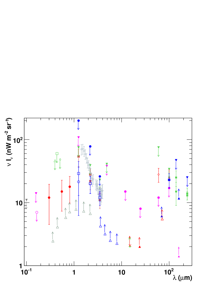
Figure 1: EBL measurements and limits. Upper limits in the UV to optical: Edelstein et al. (2000) (grey filled triangle), Martin et al. (1991) (open pink circle), Brown et al. (2000) (filled pink triangle), Mattila (1990) (open green triangle), Toller (1983) / Leinert et al. (1998) (open green square), Dube et al. (1979) / Leinert et al. (1998) (open green diamond); Tentative detection in the UV/optical: Bernstein et al. (2002, 2005) (filled red circle); Lower limits from source counts: Madau & Pozzetti (2000) (open grey triangles), Fazio et al. (2004) (open blue triangles), Elbaz et al. (2002) (green cross), Metcalfe et al. (2003) (red x), Papovich et al. (2004) (filled red triangle), Dole et al. (2006) (filled pink triangles), Frayer et al. (2006) (open red triangle); Detections in the near IR: Dwek & Arendt (1998) (open pink cross), Gorjian et al. (2000) (filled brown circle), Wright & Reese (2000) (open blue squares), Cambrésy et al. (2001) (filled brown squares), Matsumoto et al. (2005) (small open grey circles), Levenson et al. (2007) (open blue circles); Upper limits from direct measurements: Hauser et al. (1998) (filled green triangles), Dwek & Arendt (1998) (filled pink triangles), Lagache & Puget (2000) (filled blue triangles); Upper limits from fluctuation analysis: Kashlinsky et al. (1996) (filled blue circles), Kashlinsky & Odenwald (2000) (filled pink circles); Lower limits from stacking analysis in the far-IR: Dole et al. (2006) (blue triangles); Detections in the far-IR: Hauser et al. (1998) (filled green squares), Lagache & Puget (2000) (tentative, filled blue square), Finkbeiner et al. (2000) (tentative, open red diamonds).

The diffuse extragalactic background light (EBL) in the UV to far-IR wavelength regime carries important information about the galaxy and star formation history of the universe. The present EBL consists of the integrated electromagnetic radiation from all epochs, which is redshifted, corresponding to its formation epoch. In the energy density distribution, a two-peak structure is commonly expected: a first peak around 1$\,\mu$m produced by starlight and a second peak at $\sim$100$\,\mu$m resulting from starlight that has been absorbed and reemitted by dust in galaxies. Other contributions, like emission from AGN and quasars, are expected to produce no more than 5 to 20% of the total EBL density in the mid IR (see e.g. Matute et al. 2006 and references therein).

Solid lower limits for the EBL level have been derived from source counts (e.g. Madau & Pozzetti 2000; Fazio et al. 2004; Frayer et al. 2006; Dole et al. 2006). Direct measurements of the EBL have proven to be a difficult task due to dominant foregrounds mainly from inter-planetary dust (zodiacal light) (e.g. Hauser et al. 1998), and it is not expected that the sensitivity of measurements will greatly improve over the next few years. Several upper limits were reported from direct observations (e.g. Hauser et al. 1998) and from fluctuation analyses (e.g. Kashlinsky & Odenwald 2000). In total, the collective limits on the EBL between the UV and far-IR confirm the expected two-peak structure, although the absolute level of the EBL density remains uncertain by a factor of 2 to 10 (see Fig. 1). In addition, several direct detections have also been reported, which do not contradict the limits but lie significantly above the lower limits (see Hauser & Dwek 2001 and Kashlinsky 2005 for recent reviews). In particular, a diffuse residual excess in the near IR (1 to 4 $\mu$m) was reported by the IRTS satellite (Matsumoto et al. 2005), which is significantly higher than the EBL density expected from galaxy number counts.

The reported excess lead to a controversial discussion about its origin. If the excess were extragalactic origin (i.e. associated with the EBL), it might be attributed to emissions by the first stars in the history of the universe (Population III) and would make the EBL and its structure a unique probe of the epoch of Population III formation and evolution (Mapelli et al. 2004; Kashlinsky et al. 2005). Such a luminous Population III star generation, however, over-predicts the number of Ly-$\alpha$ emitters in ultra-deep field searches (Salvaterra & Ferrara 2006) and violates common assumptions on baryon consumption and star formation rates (Dwek et al. 2005a). In addition, Dwek et al. (2005a) and Matsumoto et al. (2005) point out that the NIR excess could be attributed to zodiacal light.

A different approach of deriving constraints on the EBL (labeled “clever” by Dwek & Slavin 1994) became available with the detection of very high-energy (VHE) $\gamma$-rays from distant sources (Punch et al. 1992). These VHE $\gamma$-rays are attenuated via pair production with low-energy photons from the EBL (Gould & Schréder 1967). It was soon realized that the measured spectra can be used to test the transparency of the universe to VHE $\gamma$-rays and thus to derive constraints on the EBL density (Fazio & Stecker 1970). With reasonable assumptions about the intrinsic spectrum emitted at the source, limits on the EBL density can be inferred.In a pioneering work conducted by Stecker et al. (1996), first limits on the EBL were derived. The method is, however, not straightforward. It is, in principle, not possible to distinguish between source-inherent effects (such as absorption in the source, highest particle energies, magnetic field strength, etc.) and an imprint of the EBL on a measured VHE spectrum. The emission processes in the detected extragalactic VHE $\gamma$-ray emitters are far from being fully understood, which makes it more difficult to use robust assumptions on the shape of the intrinsic spectrum. Different EBL shapes can lead to the same attenuation imprint in the measured spectra, thus a reconstructed attenuation imprint cannot uniquely be identified with one specific EBL shape. A further uncertainty arises due to the unknown evolution of the EBL with time, which becomes more important for distant sources.

Nevertheless, measured VHE $\gamma$-ray spectra can provide robust upper limits on the density and spectral distribution of the EBL, if conservative assumptions about the emission mechanisms of $\gamma$-rays are considered. A review of the various efforts to detect the EBL or to derive upper limits via the observation of extragalactic VHE $\gamma$-ray sources up to the year 2001 can be found in Hauser & Dwek (2001). The measured spectrum of the TeV blazar H 1426+428 at a redshift of $z=0.129$ (Aharonian et al. 2002b) led to a first tentative detection of an imprint of the EBL in a VHE spectrum (Aharonian et al. 2002b, 2003c). Using the H 1426+428 spectrum, together with the spectra of previously detected TeV blazars, limits on the EBL were derived (Costamante et al. 2003; Kneiske et al. 2004). Later, Dwek & Krennrich (2005) utilized a large sample of TeV blazar spectra and solid statistical methods to test a set of EBL shapes on their physical feasibility. The EBL shapes were considered forbidden, when, under the most conservative assumptions, the intrinsic spectra showed a significant exponential rise at high energies. Using the VHE spectra of the TeV blazars Mkn 421, Mkn 501, H 1426+428, and PKS 2155-304, Dwek et al. (2005b) argued that the claimed NIR excess is very unlikely to be of extragalactic origin and that an EBL density on the level of the source counts gives a good representation of the intrinsic spectra. Recently, the detection of the two distant TeV blazars H 2356-309 and 1ES 1101-232 by the H.E.S.S. experiment has been used to derive strong limits on the EBL density around 2$\,\mu$m (Aharonian et al. 2006a). The method is based on the hypothesis that the intrinsic TeV blazar spectrum cannot be harder than a theoretical limit and that the spectrum of the EBL follows a certain shape (Primack et al. 1999). To derive limits on the EBL density, the shape is scaled until the de-absorbed TeV blazar spectrum meets the exclusion criteria. The derived upper limits are only a factor of two above the lower limits from the integrated light of resolved galaxies.

In the past 2-3 years, many new TeV blazars have been discovered and the established ones were remeasured with higher sensitivity with the new Imaging Atmospheric Cherenkov Telescopes (IACT) such as H.E.S.S and MAGIC. It is therefore of high interest whether the new measurements agree with the previous limits on the EBL. Furthermore, to derive limits on the EBL from the data, it is important to scrutinize all available data together to obtain a consistent picture and to maximize the constraints. In this paper we use, therefore, spectra from all TeV blazars to derive upper limits on the EBL density in a wide wavelength range from the optical to far-infrared. Moreover, a common criticism of the EBL limits previously derived with this method is that the limits are obtained by assuming a certain EBL model and e.g. scaling it, or by exploring just a few model parameters. Since EBL models are complex and different models do not agree in details, the derived limits become very model-dependent. In order to avoid this dependency, we developed a novel technique of describing the EBL number density by spline functions, which allows us to test a large number of hypothetical EBL shapes. Our aims are to

1. Provide limits on the EBL density, which do not rely on a predefined shape or model, but rather allow for any shape compatible with the current limits from direct measurements and model predications.

2. Treat all TeV blazar spectra in a consistent way, using simple and generic assumptions about the intrinsic VHE $\gamma$-ray spectra and a statistical approach to find exclusion criteria.

3. Use spectral data from all detected TeV blazars to (a) derive upper limits on the EBL density from the individual spectra and then (b) combine these results into a single robust limit on the EBL density for a wide wavelength range.

The paper is organized as follows: In Section 2 we describe our method of using splines and a grid in EBL density vs. wavelength to construct different shapes, in Section 3 we introduce the TeV blazar spectra, and in Section 4 we describe the criteria we impose on these spectra to derive limits on the density of the EBL. In Section 5 results for individual sources and in Section 6 the combined results are discussed. Last but not least, we give a conclusion and outlook in Section 7.

Throughout the paper we adopt a Hubble constant of $H_{0}=72\,$km $s^{-1}$Mpc^-1 and a flat universe cosmology with a matter density normalized to the critical density of $\Omega_{m}=0.3$ and $\Omega_{\lambda}=0.7$.

2 Grid scan of the EBL with splines

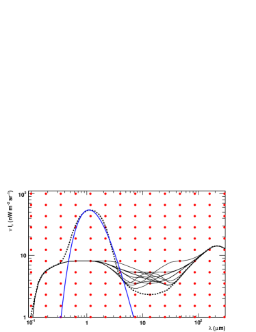
Figure 2: Examples for spline shapes resulting from the grid layout, overlaid on the grid points (red filled circles). The dashed black line illustrates the thinnest structure that can be achieved with our grid setup. A Planck spectrum (blue line) is given for comparison. Further examples for shapes are given as solid black lines.

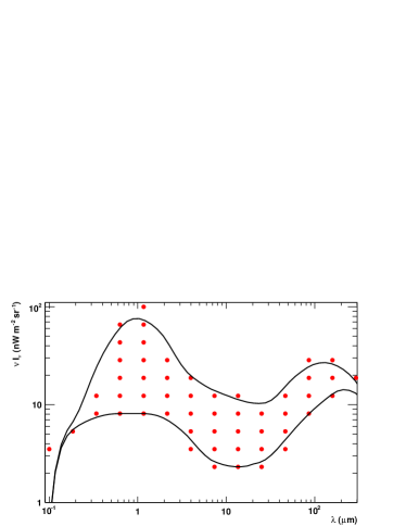
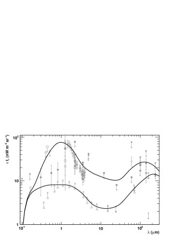
Figure 3: Top: Grid points (red filled circles) and minimum and maximum shape of the scan. Bottom: Minimum and maximum shape overlaid on the EBL measurements from Fig. 1

TeV $\gamma$-rays traversing the extragalactic radiation fields are absorbed via pair production with the low-energy photons of the EBL: $\gamma_{\rm{TeV}}\;\gamma_{\rm{EBL}}\rightarrow e^{+}\;e^{-}$. Details on the cross section (Heitler 1960) and the exact calculations can be found elsewhere (see Dwek & Krennrich 2005 for an overview). Here, we focus on the new technique using splines (as introduced below) to be able to examine as many as several million possible EBL shapes.

To calculate the optical depth $\tau_{\gamma}$ for a TeV-$\gamma$ ray of energy $E_{\gamma}$ emitted at a redshift of $z$ for one realization/shape of the EBL, one needs to solve a three-fold integral over the distance $\ell$, the interaction angles between the two photons $\mu=\cos\theta$ and the number density of the EBL photons $n_{\epsilon}$:

$$\tau_{\gamma}(E_{\gamma},\ z)=$$ (1)

$$\int_{0}^{z}{\rm d}\ell({\rm z})\int_{-1}^{+1}{\rm d}\mu\ {1-\mu\over 2}\int_{\epsilon^{\prime}_{th}}^{\infty}{\rm d}\epsilon^{\prime}\ n_{\epsilon}(\epsilon^{\prime},z)\ \sigma_{\gamma\gamma}(E^{\prime}_{\gamma},\ \epsilon^{\prime},\ \mu)$$

where $\sigma_{\gamma\gamma}$ is the pair production cross section, $\epsilon$ the energy of the EBL photon, and $E_{\gamma}^{\prime}$ and $\epsilon^{\prime}$ refer to redshifted energy values. For the large number of shapes ($\sim$8 million) we will analyze, a full numerical integration would require an extensive amount of computing power. To avoid this problem, we parametrize the EBL number density at $z=0$ as a spline

$$\ n_{\epsilon}(\epsilon)=\sum_{i=0}^{k}w_{i}s_{i,p}(\epsilon)$$ (2)

with

$$s_{i,0}(\epsilon) = \left\{\begin{array}[]{l}1\;\;\;\mbox{if}\;\epsilon_{i}\leq\epsilon<\epsilon_{i+1}\;\mbox{and}\;\epsilon_{i}<\epsilon_{i+1}\;\;\;\mbox{otherwise}\\ 0\\ \end{array}\right.$$ (5)

$$s_{i,p}(\epsilon) = \frac{\epsilon-\epsilon_{i}}{\epsilon_{i+p}-\epsilon_{i}}s_{i,p-1}(\epsilon)+\frac{\epsilon_{i+p+1}-\epsilon}{\epsilon_{i+p+1}-\epsilon_{i+1}}s_{i+1,p-1}(\epsilon)\;.$$

Here $p$ is the order of the spline and is set to $p=3$ throughout the paper, $k$ is the number of supporting points, $\epsilon_{1},...,\epsilon_{k}$ are the positions of the supporting points of the curve, and $w_{1},...,w_{k}$ are weights controlling the shape of the curve.

A way to visualize this spline is to add a number of Gaussian-like base functions to lead to a smooth curve, whereby the base functions can be weighted ($w_{i}$) to achieve different overall shapes. These base functions are characterized by a position of the center and a certain width, which depends on the order $p$ and the spacing of the supporting points.

By inserting Eq. (2) into Eq. (1) and then swapping the integration and the summation, one obtains an expression for the optical depth, where the integral can be solved easily for a certain redshift and set of supporting points of the spline. The optical depth can then be calculated by a simple summation, where the shape of the EBL is determined by the choice of a set of weights.

To estimate the numerical uncertainties in the integration of the base functions, the result for $\tau_{\gamma}$ from the summation is compared to the results from a full integration over the actual EBL shapes for several shapes and spectra used in this paper. The deviation for almost all settings is found to be less then 0.5%. Even for extreme cases (high redshift, high EBL density), the deviation is always less than 2%. These small deviations arise from inaccuracies in the numerical integration of the base functions.

The spline parameterization is used to construct a set of EBL shapes using a grid in EBL energy density vs. wavelength. The x-positions of the grid points (wavelength) are used as positions for the supporting points $\epsilon_{i}$ of the spline. The y-positions of the grid points (energy density) are used as weights $w_{i}$.

For the supporting points (x-axis of the grid) $\epsilon_{i}$, we use 16 equidistant points in $\log_{10}(\lambda)$ ($\lambda=hc/\epsilon$) from 0.1 to 1000$\,\mu$m. The number and distance of the supporting points, together with the order of the spline, determines the width of the structures, which can be described with the spline. Given the grid setup and the spline of order $p=3$, the thinnest peak or dip that can be modeled is about three grid points wide (Fig. 2). This minimum width is similar to a Planck spectrum from a black body radiation (Fig. 2). It is expected that the EBL originates mainly from an overlap of the redshifted spectra of single stars, for which a Planck spectrum is a good first-order approximation, and dust reemission. Thus, an EBL structure thinner than a Planck spectrum is unlikely.

Noteworthy, any extremely sharp and strong cut-offs or bumps can only be described in an approximate way. Such features can arise from the Lyman-$\alpha$ drop-off of massive Population III stars in certain models (e.g. Salvaterra & Ferrara 2003), but they are generally not expected on larger wavelength scales, since they would be smoothed out by redshift. Of course the upper limits depend on the thickness of the structures modeled, and the choice of minimum thickness has to be physically motivated, as it is in our case.

The weights $w_{i}$ of the spline (y-axis of the grid) are varied in 12 equidistant steps in $\log_{10}$(energy density) from 0.1 to 100 nW m${}^{-2}\,$sr^-1. Since we apply the grid point positions directly as weights $w_{i}$, the resulting curve does not directly go through the grid points. So for all limits, etc., the actual curve has to be considered and not the grid point positions. Our use of the grid point positions as weights also results in several shapes lying between two grid points. This is illustrated in Fig. 2 for two arbitrarily chosen grid points between 10 and 20$\,\mu$m.

For the scan, a subset of grid points is selected such that all resulting shapes are within the limits given by the galaxy counts on the lower end and by the limits from the direct measurements and the fluctuation analyses on the upper end. In the 20 to 100$\,\mu$m regime, we choose a somewhat looser shape, given the wider spread of the (tentative) measurements (Fig. 3). By iterating over all grid points, we obtain 8 064 000 different EBL shapes, which will be examined.

The generic shapes used in this analysis have no redshift dependency, thus evolution of the EBL cannot be taken into account. We assume a constant photon number density only expanding and shifting in wavelength with expansion of the universe. Neglecting the evolution of the EBL is a valid assumption for nearby sources (e.g. Mkn 501), but for distant sources this can result in an additional error in the order of 10 to 20% depending on the evolution model and redshift (see e.g. Aharonian et al. 2006a). The possible systematic error arising from this assumption will be discussed further in Sect. 7.

For a given optical depth $\tau_{\gamma}(E_{\gamma},\,z)$ one can determine the intrinsic differential energy spectrum using

$$dN/dE_{\mathrm{intr.}}\,=\,dN/dE_{obs}\times\exp[\tau_{\gamma}(E_{\gamma},\,z)],$$ (6)

where $dN/dE_{obs}$ is the observed spectrum. The intrinsic spectrum is then tested on its physical feasibility as described in Section 4. This process is repeated for all VHE $\gamma$-ray sources (described in the next section) and for all 8 064 000 EBL shapes.

3 TeV blazar sample

Table 1: TeV blazar spectra used in this paper.

Source	Redshift	Experiment	Energy range	Slope	Cut-off energy	Reference
			(TeV)	$\Gamma\pm\sigma_{\mathrm{st}}\pm\sigma_{\mathrm{sy}}$	(TeV)
Mkn 421	0.030	MAGIC	0.10 – 3.0	$2.20\pm 0.08\pm 0.20$	$1.44\pm 0.28$	Albert et al. (2007b)
Mkn 421	0.030	HEGRA	0.70 – 18.0	$2.19\pm 0.02\pm 0.20$	$3.6+0.4-0.3$	Aharonian et al. (2002a)
Mkn 421	0.030	Whipple	0.35 – 0.90	$2.31\pm 0.04\pm 0.05$	——	Krennrich et al. (2002)
Mkn 501	0.034	HEGRA	0.50 – 22.0	$1.92\pm 0.03\pm 0.20$	$6.2\pm 0.4$	Aharonian et al. (1999)
1ES 2344+514	0.044	Whipple	0.80 – 11.0	$2.54\pm 0.17\pm 0.07$	——	Schroedter et al. (2005)
Mkn 180	0.045	MAGIC	0.14 – 1.5	$3.25\pm 0.66\pm 0.20$	——	Albert et al. (2006b)
1ES 1959+650	0.047	HEGRA	1.5 – 13.0	$2.83\pm 0.14\pm 0.08$	——	Aharonian et al. (2003a)
PKS 2005-489	0.071	H.E.S.S.	0.20 – 2.5	$4.0\pm 0.4\,(\pm 0.2)$	——	Aharonian et al. (2005a)
PKS 2155-304	0.116	H.E.S.S.	0.20 – 3.5	$3.37\pm 0.07\pm 0.10$	——	Aharonian et al. (2005b)
H 1426+428	0.129	HEGRA	0.70 – 12.0	$2.6\pm 0.6\pm 0.1$	——	Aharonian et al. (2003c)
H 2356-309	0.165	H.E.S.S.	0.16 – 1.0	$3.06\pm 0.21\pm 0.10$	——	Aharonian et al. (2006b)
1ES 1218+304	0.182	MAGIC	0.08 – 0.7	$3.0\pm 0.4\pm 0.6$	——	Albert et al. (2006a)
1ES 1101-232	0.186	H.E.S.S.	0.16 – 3.3	$2.88\pm 0.14\pm 0.1$	——	Aharonian et al. (2006a)

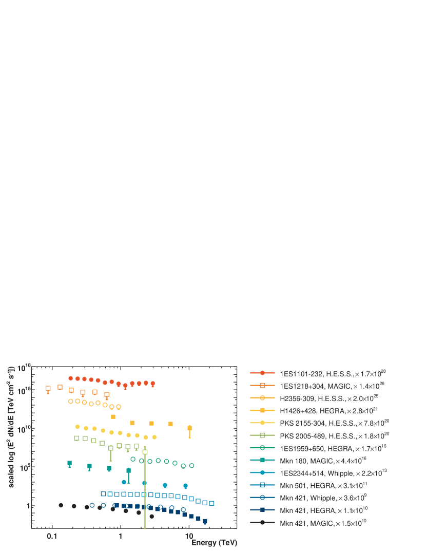
Figure 4: TeV blazar sample chosen for this study. From all detected TeV blazars, at least one spectrum is shown with the exception of PG 1553+113 (unknown redshift). The spectra are multiplied by E² to emphasize spectral differences and are spread out along the Y-axis and ordered in redshift to avoid cluttering of the plot (the corresponding scaling factors are given in the legend of the plot).

Since the detection of the first extragalactic VHE $\gamma$-ray source in 1992 (Punch et al. 1992), a wealth of new data from this source type has become available. Up to now all detected VHE $\gamma$-ray sources belong to the class of active galactic nuclei (AGN) and, with the only one exception of the radio galaxy M 87 (Aharonian et al. 2003b, 2006d), to the subclass of TeV blazars (Horan & Weekes 2004). AGNs are known to be highly variable sources, with variations of the absolute flux levels in the TeV range by more than an order of magnitude and on time scales as short as 15 min (e.g. Gaidos et al. 1996; Aharonian et al. 2002a). Changes in the spectral shapes have also been observed (e.g. Krennrich et al. 2002; Aharonian et al. 2002a).

In this study we utilize spectral data obtained during the past seven years by four different experimental groups operating ground-based imaging atmospheric Cherenkov telescopes (IACTs): Whipple (Finley & The VERITAS Collaboration 2001), HEGRA (Daum et al. 1997), H.E.S.S. (Hinton 2004) and MAGIC (Cortina et al. 2005). We select at least one spectrum for every extragalactic source with known redshift. If there is more than one measurement with a comparable energy range, we take the spectrum with the better statistics and the harder spectrum (expected to give stronger constraints, see Sect. 4). If different measurements of one source cover different energy ranges, we include both spectra as independent tests. Another possibility would be to combine the measurements from different experiments, as was done before in the case of H 1426+428 (Aharonian et al. 2003c). However, since the sources are known to be variable in the flux level and spectral shape, a combination of non-simultaneous data is not trivial. In addition, in a conservative approach one has to consider the systematic errors reported by the individual experiments, which are around 20%. Our method is quite sensitive to the errors of the flux, and this additional error would weaken our results. We therefore do not use combined spectra. The selected TeV blazar spectra are summarized in Fig. 4 and Table 1. In the case the measured spectrum can be described well by a simple power law $dN/dE\propto E^{-\Gamma}$, only the slope $\Gamma$ is quoted. Otherwise, the cut-off energy $E_{\mathrm{coff}}$ according to $dN/dE\propto E^{-\Gamma}\,\exp(-E/E_{\mathrm{coff}})$ is also quoted. If no systematic error in the photon index is given in the corresponding paper, we use a value of 0.2 (values in brackets). In Fig. 4 the spectra are multiplied by E² to emphasize spectral differences and are spread out along the Y-axis and ordered in redshift to avoid cluttering the plot.

We did not include data from the radio galaxy M 87, which was recently confirmed as a VHE $\gamma$-ray emitter (Aharonian et al. 2006d). M 87 is a nearby source ($z=0.00436$), so even for high EBL densities the attenuation is weak and would only be noticeable at high energies $\sim$30 TeV. Nevertheless, M 87 has a hard spectrum with a photon index of $\Gamma\sim 2.2$ currently measured up to 20 TeV, so further observations that extend the energy range to even higher energies could make M 87 an interesting target for EBL studies as well.

The cross section $\sigma_{\gamma\gamma}$ of the pair production process has a distinct peak close to the threshold. The maximum attenuation of VHE photons of energy $E_{\gamma}$ occurs by interaction with low-energy photons with a wavelength

$$\lambda^{\mathrm{max}}(\mu\mathrm{m})\approx 1.24\;E_{\gamma}(\mathrm{TeV}).$$ (7)

Since the selected spectra cover an energy region from 100 GeV up to more than 20 TeV, the EBL wavelength range for the absorption of VHE $\gamma$-rays spans from UV ($\sim$0.1$\,\mu$m) to the mid IR ($\sim$30$\,\mu$m). This region is of particular cosmological interest since it might contain a signature of Population III stars.

4 Exclusion criteria for the EBL shapes

Table 2: Analytical functions that are used to fit the intrinsic TeV blazar spectrum.

#	Description	Abbreviation	Formula $f(E)=dN/dE$	Parameters to evaluate
1	simple power law	PL	$N_{0}E^{-\Gamma}$	$\chi^{2},\,\Gamma^{\mathrm{PL}}$
2	broken power law with transition region	BPL	$N_{0}E^{-\Gamma_{1}}\left[1+\left(\frac{E}{E_{b}}\right)^{f}\right]^{\frac{\Gamma_{1}-\Gamma_{2}}{f}}$	$\chi^{2},\,\Gamma_{1}^{\mathrm{BPL}},\,\Gamma_{2}^{\mathrm{BPL}}$
3	broken power law with transition region and super-exponential pile-up	BPLSE	$N_{0}E^{-\Gamma_{1}}\left[1+\left(\frac{E}{E_{b}}\right)^{f}\right]^{\frac{\Gamma_{1}-\Gamma_{2}}{f}}\exp\left(\frac{E}{E_{\mathrm{p}}}\right)$	$\chi^{2}$
4	double broken power law with transition regions	DBPL	$N_{0}E^{-\Gamma_{1}}\left[1+\left(\frac{E}{E_{b1}}\right)^{f_{1}}\right]^{\frac{\Gamma_{1}-\Gamma_{2}}{f_{1}}}\left[1+\left(\frac{E}{E_{b2}}\right)^{f_{2}}\right]^{\frac{\Gamma_{2}-\Gamma_{3}}{f_{2}}}$	$\chi^{2},\,\Gamma_{1}^{\mathrm{DBPL}},\,\Gamma_{2}^{\mathrm{DBPL}},\,\Gamma_{3}^{\mathrm{DBPL}}$
5	double broken power law with transition regions and super-exponential pile-up	DBPLSE	DBPL $\times\exp\left(\frac{E}{E_{\mathrm{p}}}\right)$	$\chi^{2}$

We aim to construct an upper limit on the EBL density using the TeV blazar sample described in Sect. 3. In order to achieve this, we examine every EBL shape (as introduced in Sect. 2) to see whether the intrinsic TeV blazar spectra, which result from correcting the measured spectra for the corresponding optical depths, are physically feasible. EBL shapes are considered to be allowed if the intrinsic spectra of all tested TeV blazars are feasible. As an upper limit we define the upper envelope of all allowed shapes. It is constraining in the wavelength range where it lies below the maximum shape of the scan. Otherwise no upper limit is quoted.

There are different ways to examine a TeV blazar spectrum upon its feasibility. In this paper we follow very general arguments arising from the shock acceleration scenario of relativistic particles. In this well-accepted view, electrons are Fermi-accelerated with a resulting power-law spectrum of $dN/dE\sim E^{-\alpha}$, with a slope $\alpha$ of about 2. Due to a faster cooling of high energy electrons compared to lower energies, the slope $\alpha$ can be steeper than 2, but there is no simple theoretical possibility to produce an electron spectrum with a harder spectrum. Given an electron spectrum, one can calculate the slope of the synchrotron energy spectrum: it is $dN/dE\sim E^{-\Gamma}$ with a photon index $\Gamma=\frac{\alpha+1}{2}=1.5$. The energy spectrum of inverse-Compton photons, independent of the origin of the target photons, has approximately the same photon index as the synchrotron energy spectrum if the scattering occurs in the Thomson regime. In the case of the Klein-Nishima regime, the index is even larger. Thus, the photon index of the energy spectrum of VHE photons originating from an IC scattering is $\Gamma=1.5$ or larger. In the case of a hadronic origin, their spectrum is more complicated. Yet, the resulting VHE photons originate from pion decays leading to a photon spectrum with $\Gamma=2$, which is softer than a possible photon spectrum with a leptonic origin. In conclusion, we assume that the photon index $\Gamma$ of the intrinsic TeV blazar spectrum is 1.5 or larger. These arguments were recently used in Aharonian et al. (2003c, 2006a, 2006c) and Albert et al. (2007a).

However, a possibility of obtaining even harder photon spectra is not fully excluded. For instance, though contrary to the wide acceptance of these general arguments, Katarzyński et al. (2006) argue that synchrotron emission, as well as IC scattering of relativistic electrons, does not necessarily occur close to the region of electron acceleration. If so, the electron spectrum can become truncated due to propagation effects; i.e. the minimum energy of electrons can be as high as several GeV. In an extreme case, we deal with a monoenergetic spectrum of VHE relativistic electrons. Then, and this is the most extreme case, a resulting IC photon index can be as small as $\Gamma=2/3$. We use this limit in the present paper, in addition to the standard limit of $\Gamma=1.5$, to demonstrate the strength of our method.

In the simplest models, it is assumed that VHE photons originate from a single compact region (so-called one-zone scenario). This result in a smooth, convex spectral energy-distribution with two peaks at certain energies in a $\log(\nu F(\nu))\mathrm{vs.}\log(\nu)$ representation. Yet there are no obvious arguments against scenarios including some kind of multizone models, which can be naturally realized in the jets of TeV blazars. Then, the measured spectrum of VHE $\gamma$-ray emitting sources will be a superposition of several one-zone emission regions. So far, there has been no indication of this in the measured spectra, however, the attenuation of VHE $\gamma$-rays by EBL photons could hide such substructures.

In addition to the constraints on the photon index of the intrinsic TeV blazar spectra, we also argue that a super-exponentially rising energy spectrum with an increasing energy is not realistic. The so-called pile-up at high energies was first noticed by Protheroe & Meyer (2000) for the Mkn 501 spectrum, and early attempts to avoid it invoked violation of the Lorentz invariance (Kifune 1999; Protheroe & Meyer 2000). On the other hand, Stecker & Glashow (2001) argue that the same Mkn 501 spectrum data can be used to place severe constraints on the Lorentz-invariance breaking parameter. Another possibility for explaining pile-ups would require an ultrarelativistic jet with a very high bulk-motion Lorentz factor $\Gamma_{0}>3\times 10^{7}$ (Aharonian et al. 2002c). The pile-ups, however, seem to arise at different energies for different sources, which is not expected in these models. Moreover, the pile-ups can be easily avoided by choosing a sufficiently low level of the EBL density.

Based on the arguments above and including possible multizone emission scenarios, we assume that at least one of the following smooth, analytical functions can describe the intrinsic spectrum satisfactory well: a simple power law (PL), a broken power law with a transition region (BPL), a broken power law with a transition region and a super-exponential pile-up (BPLSE), a double broken power law with two transition regions (DBPL), or a double broken power law with two transition regions and a super-exponential pile-up (DBPLSE). The functions are summarized in Table 2.

In our approach of examining the intrinsic spectra of TeV blazars, we adopt a general assumption that one of the smooth functions above describes the intrinsic spectrum satisfactorily. In case we fail to find such a function, we abandon any further examination of the fit parameters, and a given EBL shape (realization) is not excluded. It is noteworthy that less than 0.06% of all intrinsic spectra of the TeV blazars could not be fitted well by the chosen functional forms, which are described below.

In order to determine a good analytic description, we fit the intrinsic spectrum with the functions listed above, starting with the simplest one (PL). As “good description” we take a fit with a chance probability $P_{\mathrm{Fit}}>$ 5% based on its $\chi^{2}$ value. The determined fit parameters are examined to be physically meaningful as described below. If the fit has a probability $P_{\mathrm{Fit}}<$ 5%, we do not consider the function and examine the next function from the list (Table 2). Also if the fit has a chance probability $P_{\mathrm{Fit}}>$ 5%, but the determined parameters do not lead to an exclusion of the corresponding EBL shape, we take the next function from the list. The reason is that a function with more free parameters can lead to a significantly better fit. In order to make sure that a more complicated function indeed describes the intrinsic shape better than a simpler one, we use the likelihood ratio test (Eadie et al. 1988, Appendix A). We require at least a 95% probability to prefer a function with a higher number of free parameters. Only if the function is preferred, we examine its fitted parameters and their errors. Spectra with $n$ data points are only fitted with functions with up to $n-1$ parameters. In case of spectra with low statistics, we fix the softness of the break ($f$, see Table 2) between two spectral indices to an a priori chosen value of $f=4$ to allow for a fit by a higher-order function (e.g. in case of the BPL for H 1426+428).

We finally define the following criteria to exclude an assumed EBL shape:

• At least one of the determined photon indices from the best hypothesis is outside of the allowed range, i.e. $\Gamma^{i,\mathrm{max}}<\Gamma^{\mathrm{limit}}$, where $\Gamma^{\mathrm{limit}}=1.5$ or 2/3, and $\Gamma^{i,\mathrm{max}}=\Gamma^{i}+\sigma_{\Gamma^{i}}+\sigma_{\mathrm{sy}}$ with $\Gamma^{i}$ and $\sigma_{\Gamma}$ the fitted photon index and its error, respectively, and $\sigma_{\mathrm{sy}}$ as the systematic error on the spectral slope (as given for the corresponding measurement).

• The best fit is obtained by one of the two shapes with an exponential pile-up (BPLSE or DBPLSE).

A single confidence level for the derived upper limits on the EBL density cannot be quoted easily: For the test on the photon index we use a 1 $\sigma$ confidence level (as defined for two-sided distributions, including systematic errors). For the likelihood ratio test, we use a 2 $\sigma$ level (as defined for one-sided distributions). Thus, the confidence level for the upper limit ranges from 68% to 95%.

As discussed in this section, the theoretical expectations on the smallest possible photon index $\Gamma^{\mathrm{limit}}$ have a given spread. Thus, we perform two EBL scans, assuming a limit of $\Gamma^{\mathrm{limit}}=1.5$ for the first realistic case and for the second extreme case a limit of $\Gamma^{\mathrm{limit}}=2/3$. From here on, we refer to realistic and extreme scan accordingly.

Since our exclusion criteria consider the effect of an EBL shape solely on the hardness of the spectra of extragalactic VHE $\gamma$-ray sources, some shapes might be considered viable in our scan, even though other criteria for exclusion could be found (e.g. exclusion based on spectral shape of the EBL, related to the energy density of star and dust emission as discussed in Dwek & Krennrich 2005). In this respect our approach is conservative.

5 Results for individual spectra

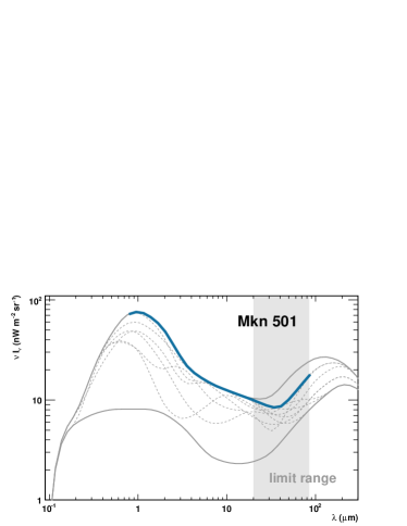
Figure 5: Limits on the EBL density from Mkn 501 ($\Gamma_{\mathrm{max}}>1.5$). Grey solid curves are the minimum and maximum shapes of the scan; grey dashed curves are all the highest allowed EBL shapes for Mkn 501; the thick colored curve is the corresponding envelope shape. The grey shaded area marks the wavelength region, in which the envelope shape is constraining the EBL density.

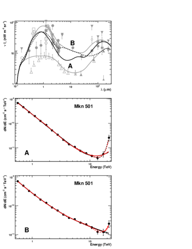
Figure 6: Mkn 501 individual results ($\Gamma_{\mathrm{max}}>1.5$). Upper Panel: Two examples for the highest allowed shapes (A - solid line; B - dashed line) overlayed on EBL measurements and the minimum and maximum shapes of the scan (grey). Middle Panel: Intrinsic spectrum for shape A and fit functions: BPL (solid black line), BPLSE (solid red line), DBPL (dashed black line), and DBPLSE (dashed red line). The fit parameters can be found in Table 3. The BPL and BPLSE are not good fits; the DBPL is a good fit and its parameters are within the allowed range; the DBPLSE is not prefered over the BPL and the DBPL. Lower Panel: Intrinsic spectrum for shape B and the same fit functions as in the Middle Panel. The fit parameters can be found in Table 3. All four functions are good fits. No function is preferred over the BPL.

Table 3: Fit results for the Mkn 501 spectrum using the functions from Fig. 6.

	$P_{\mathrm{Fit}}$	Pref.	$\Gamma_{\mathrm{1,max}}$	$\Gamma_{\mathrm{2,max}}$	$\Gamma_{\mathrm{3,max}}$
Shape A
BPL	0.00	—	(2.13)	(-0.47)	—
BPLSE	0.04	—	—	—	—
DBPL	0.19	yes	2.12	1.62	8.92
DBPLSE	0.40	no	—	—	—
Shape B
BPL	0.16	yes	2.85	1.77	—
BPLSE	0.23	no	—	—	—
DBPL	0.12	no	(3.91)	(1.42)	(1.05)
DBPLSE	0.24	no	—	—	—

Figure 7: Limits on the EBL density from H1426+428 ($\Gamma_{\mathrm{max}}>1.5$). Grey solid curves are the minimum and maximum shapes of the scan; grey dashed curves are all the highest allowed EBL shapes for H1426+428; the thick colored curve is the corresponding envelope shape. The grey shaded area marks the wavelength region, in which the envelope shape is constraining the EBL density.

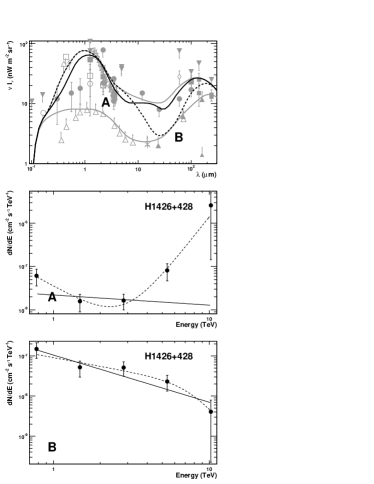
Figure 8: H1426+428 individual results ($\Gamma_{\mathrm{max}}>1.5$). Upper Panel: Two examples for the highest allowed shapes (A - solid line; B - dashed line) overlayed on EBL measurements and the minimum and maximum shapes of the scan (grey). Middle Panel: Intrinsic spectrum for shape A and fit functions. Both PL (solid line) and BPL (dashed line) are good fits; $\Gamma_{\mathrm{max}}^{\mathrm{PL}}=0.23+1.18_{\mathrm{stat}}+0.2_{\mathrm{sys}}=1.61$, and the BPL fit is preferred over the PL fit ($P_{\mathrm{(BPL\;vs.\;PL)}}=0.97$); $\Gamma_{\mathrm{1,max}}^{\mathrm{BPL}}=2.01+1.94_{\mathrm{stat}}+0.2_{\mathrm{sys}}=4.15$ and $\Gamma_{\mathrm{2,max}}^{\mathrm{BPL}}=-4.59+6.67_{\mathrm{stat}}+0.2_{\mathrm{sys}}=2.28$. Lower Panel: Intrinsic spectrum for shape B and fit functions. Both PL (solid line) and BPL (dashed line) are good fits; $\Gamma_{\mathrm{max}}^{\mathrm{PL}}=1.18+0.24_{\mathrm{stat}}+0.2_{\mathrm{sys}}=1.63$ and the BPL fit is not preferred over the PL fit ($P_{\mathrm{(BPL\;vs.\;PL)}}=0.54$);

Figure 9: Limits on the EBL density from 1ES 1101-232 ($\Gamma_{\mathrm{max}}>1.5$). Grey solid curves are the minimum and maximum shapes of the scan; grey dashed curves are all the highest allowed EBL shapes for 1ES 1101-232; the thick colored curve is the corresponding envelope shape. The grey shaded area marks the wavelength region, in which the envelope shape is constraining the EBL density.

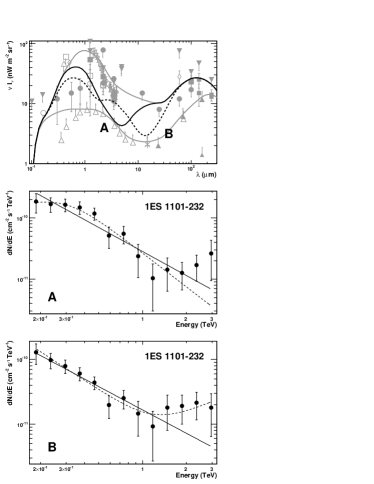
Figure 10: 1ES 1101-232 individual results ($\Gamma_{\mathrm{max}}>1.5$). Upper Panel: Two examples for the highest allowed shapes (A - solid line; B - dashed line) overlayed on EBL measurements and the minimum and maximum shapes of the scan (grey). Middle Panel: Intrinsic spectrum for shape A and fit functions. Both PL (solid line) and BPL (dashed line) are good fits; $\Gamma_{\mathrm{max}}^{\mathrm{PL}}=1.31+0.13_{\mathrm{stat}}+0.1_{\mathrm{sys}}=1.53$ and the BPL fit is not preferred over the PL fit ($P_{\mathrm{(BPL\;vs.\;PL)}}=0.87$). Lower Panel: Intrinsic spectrum for shape B and fit functions. Both PL (solid line) and BPL (dashed line) are good fits; $\Gamma_{\mathrm{max}}^{\mathrm{PL}}=1.21+0.21_{\mathrm{stat}}+0.1_{\mathrm{sys}}=1.52$ and the BPL fit is not preferred over the PL fit ($P_{\mathrm{(BPL\;vs.\;PL)}}=0.9488$).

To present the results for individual spectra in a compact and non-repetitive way, we sort our preselected spectra into three categories. For each category we select one prototype spectrum (following similar criteria to those in Sect. 3), for which we give results. The categories considered are:

”Nearby and well-measured”.

As prototype spectrum we select the Mkn 501 spectrum ($z=0.034$) recorded by HEGRA during a major TeV flare in 1997. The relatively hard spectrum provides good statistics from 800 GeV up to 25 TeV. Other sources in this category are Mkn 421 and 1ES 1959+650. 1ES 2344+514 and Mkn 180 are at a comparable distance, but the spectra do not have such high statistics. PKS 2005-489 lies somewhere between this and the following category. Spectra in this category mainly provide limits in the FIR due to a pile-up at high energies.

”Intermediate distance, wide energy range”.

The prototype for this category is the spectrum from H 1426+428 at a redshift of $z=0.129$, with energies ranging from 700 GeV up to 12 TeV. PKS 2155-304 is at a comparable distance, and its measured spectrum has a better statistic, but the highest energy point is only at 2.5 TeV; and the spectrum is much softer.

”Distant source, hard spectrum”.

The most distant TeV blazar discovered so far with a published energy spectrum is 1ES 1101-232 at a redshift of $z=0.186$. Its spectrum is hard and ranges from 160 GeV to 3.3 TeV. H 2356-309 and 1ES 1218+304 are at similar distances, but the statistics are not as good and/or the spectrum is softer. This makes 1ES 1101-232 the natural choice for a prototype spectrum in this category.

As the limit on the EBL for the individual spectra (and for the combined results in Sect. 6 as well), we define the envelope shape of all allowed EBL shapes. In most cases a single EBL shape represents the highest allowed shape only for a small wavelength interval. Consequently the envelope shape consists of a number of segments from different EBL shapes. One exception occurs, if the maximum shape tested in the scan is allowed. In this case the spectrum does not constrain the EBL density. In general, a spectrum constrains the EBL density when the envelope shape lies below the maximum shape tested in the scan.

Given the energy range of the spectra, the limit is only valid for wavelengths $\lambda_{\mathrm{Lim}}$:

$$\lambda^{\mathrm{max}}(E_{min})\;<\;\lambda_{\mathrm{Lim}}\;<\;\lambda^{\mathrm{thresh}}(E_{max})$$ (8)

where $\lambda^{\mathrm{max}}(E_{min})$ is the wavelength for which the cross section for pair production with the lowest energy point of the VHE spectrum $E_{min}$ is maximized (following Eqn. (7)). The variable $\lambda^{\mathrm{thresh}}(E_{max})$ is the threshold wavelength for pair production with the highest energy point of the VHE spectrum $E_{max}$. This wavelength range roughly reflects the sensitivity of the exclusion criteria. There is, of course, some freedom of choice for the wavelength range, given the complexity of the criteria.

In the following three sections the results for the individual prototype spectra for the realistic scan with $\Gamma_{\mathrm{max}}>1.5$ are summarized. The results for the extreme scan with $\Gamma_{\mathrm{max}}>2/3$ for all prototype spectra are presented in Sect. 5.4.

5.1 Nearby and well-measured: Mkn 501 (HEGRA)

The envelope shape derived for the Mkn 501 spectrum is shown in Fig. 5 in comparison with the maximum and minimum EBL shapes tested in the scan. Although 7 766 674 out of 8 064 000 EBL shapes (96.3%) can be excluded, the effective limit is only constraining in the 20 to 80$\,\mu$m wavelength region, where it lies below the maximum tested shape. Note that our method is not only testing the overall level of the EBL density but is also sensitive to its structures. Despite the fact that, for the Mkn 501 spectrum, almost all of the tested EBL shapes are excluded, certain types of shapes are allowed, independent of their respective EBL density level. This can be illustrated with an EBL shape, which has a power law dependency $n(\epsilon)\sim\epsilon^{-1}$ or $\nu I_{\nu}\sim\lambda^{-1}$. Then the optical depth is independent of the energy of VHE photons and the intrinsic TeV blazar spectrum has the same shape as the observed one (Aharonian 2001). With such a type of shape, an allowed high EBL density level in the MIR can be constructed by choosing a corresponding high density level in the optical/NIR.

The rejection power in the FIR results mainly from the hard intrinsic Mkn 501 spectrum above $\sim$5 TeV that often can only be described by an exponential or super exponential rise. Two of the limiting shapes, together with the resulting intrinsic spectra and fit functions, are shown in Fig. 6 and the corresponding fit results can be found in Table 3. In the table, the fit probabilities are given in the column “$P_{\mathrm{Fit}}$”. The parameters are put in parentheses, if the corresponding fit has a low probability or it is not preferred over a fit by a function with less free parameters (result of the likelihood ratio test, indicated in the column “Pref”). The fit with a PL function did not meet our acceptance criteria, and the function is omitted from the figure for the sake of legibility. For the two shapes displayed here, the pile up at high energies is already visible but not yet significant.

5.2 Intermediate distance, wide energy range: H1426+428

Using the H 1426+428 energy spectrum 5 571 772 EBL shapes (corresponding to 69.09% of all shapes) are excluded. The resulting envelope shape is displayed in Fig. 7, together with all highest allowed shapes. The limit is constraining from $\sim$6 to $\sim$20$\,\mu$m and the constraints are not very strong. This is illustrated in Fig. 8, where two representative highest allowed EBL shapes and the resulting intrinsic spectra are shown, as are the relevant fit functions. Shape A is almost as high as the maximum shape of the scan. Although the intrinsic spectrum is already convex, the relative low statistics of the spectrum even allows for an acceptable fit by a simple PL and results in large errors on the fit parameters for the BPL. Consequently the EBL shape cannot be excluded. Shape B has a high peak in the O/IR wavelength region but lies below all upper limits in the FIR. The resulting intrinsic spectrum is best described with a simple PL with a maximum slope $\Gamma_{\mathrm{max}}^{\mathrm{PL}}=1.63>1.5$ and is therefore allowed.

5.3 Distant source, hard spectrum: 1ES 1101-232

The spectrum from 1ES 1101-232 gives the strongest constraints for all individual spectra, even though slightly less EBL shapes (7 706 625, 95.57% of all shapes) are excluded than in the case of Mkn 501. This is due to the different sensitivities in EBL wavelength; the 1ES 1101-232 spectrum is only sensitive up to  10$\,\mu$m. The resulting maximum shapes and the envelope shape are shown in Fig. 9. The envelope shape constraints the EBL density in the wavelength range from $\sim$0.4 to $\sim$10$\,\mu$m and clearly excludes the NIR excess claimed by Matsumoto et al. (2005) as being extragalactic. At EBL wavelengths of $\sim$2$\,\mu$m the limit is consistent with the limit derived by Aharonian et al. (2006a) for the same source with a different technique (see Sect. 6). Two representative highest allowed shapes and the corresponding intrinsic spectra are shown in Fig. 10. Shape A illustrates the intrinsic spectrum for a high EBL density in the UV/O, while shape B is the maximum shape for wavelengths around 3$\,\mu$m. For both shapes the examined fit parameters are close to the allowed limits (see caption for values), as expected for highest allowed shapes.

5.4 Extreme case: $\Gamma_{\mathrm{max}}>2/3$

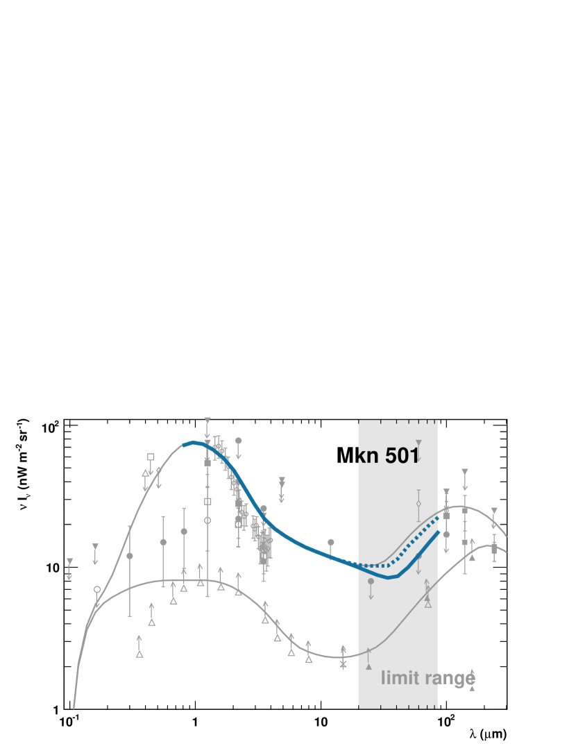
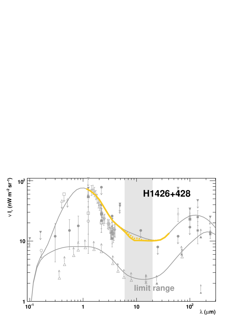
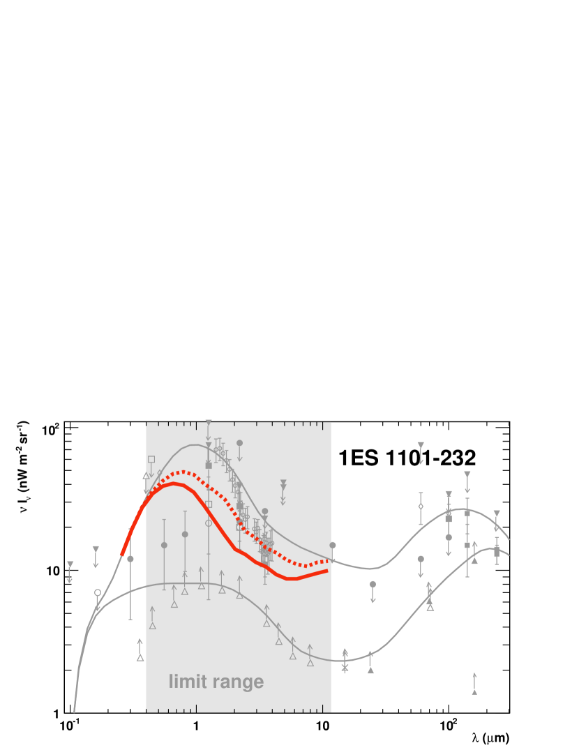
Figure 11: Result for individual spectra, comparing the realistic case with $\Gamma_{\mathrm{max}}>1.5$ (thick colored solid line) with the extreme case with $\Gamma_{\mathrm{max}}>2/3$ (thick colored dashed line), overlaid on the EBL measurements and the minimum and maximum shapes of the scan (grey markers and lines). The grey boxes indicate the validity range of the limit for the realistic scan as in Figs. 5, 7, and 9. Note that the validity range of the limits from the extreme scan are quite similar. Upper Left Panel: Results for Mkn 501 (HEGRA). Upper Right Panel: Results for H1426+428. Lower Left Panel: Results for 1ES 1101-232.

The upper limits for Mkn 501, H1426+428 and 1ES 1101-232 for the extreme case with $\Gamma_{\mathrm{max}}>2/3$ are shown in Fig. 11 in comparison to the limits derived for the realistic case. In the case of Mkn 501, a similar number of EBL shapes (94.13%) as in the realistic scan are excluded, but the effective limit is less constraining (Fig. 11, Upper Left Panel). For H1426+428 the limit almost remains at the same level, still close to the maximum shape tested in the scan (Fig. 11, Upper Right Panel). For 1ES 1101-232 the limit in the UV/O lies a factor of 1.2 to 1.8 higher than the limit in the realistic case (Fig. 11, Lower Left Panel). In the wavelength region from 2 to 4$\mu$m, the NIR excess claimed by Matsumoto et al. (2005) is now compatible with the limit. In the 1 to 2$\mu$ region the limit still lies clearly below the claimed NIR excess.

6 Combined results

Table 4: Number of excluded EBL shapes for the realistic scan for individual spectra (column two) as well as the number of the intrinsic spectra, which could not be fitted satisfactorily (column three).^a

Spectrum	#Shapes Excluded	#Shapes No Fit
Mkn 421 (MAGIC)	1 756 869 (21.79%)	59 258 (0.94%)
Mkn 421 (HEGRA)	888 575 (11.02%)	0
Mkn 421 (Whipple)	2 287 059 (28.36%)	0
Mkn 501	7 760 733 (96.24%)	1296 (0.43%)
1ES 2344+514	0	0
Mkn 180	0	0
1ES 1959+650	1 086 314 (13.47%)	423 (0.01%)
PKS 2005-489	0	0
PKS 2155-304	4 248 872 (52.69%)	0
H 1426+428	5 571 771 (69.09%)	2 (0.00%)
H 2356-309	4 657 817 (57.76%)	0
1ES 1218+304	19 540 (00.24%)	0
1ES 1101-232	7 706 624 (95.57%)	0

^a The percentage of these numbers to the number of all shapes (8 064 000) for column two and to the number of the allowed shapes for this spectrum for column three is also quoted. If the number of shapes is zero, the percentage is omitted.

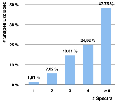
Figure 12: Number of excluded shapes as percentage of the total number of shapes vs. the number of spectra, that excluded the shape. A large fraction of shapes (98.08%) is excluded by more than one spectra.

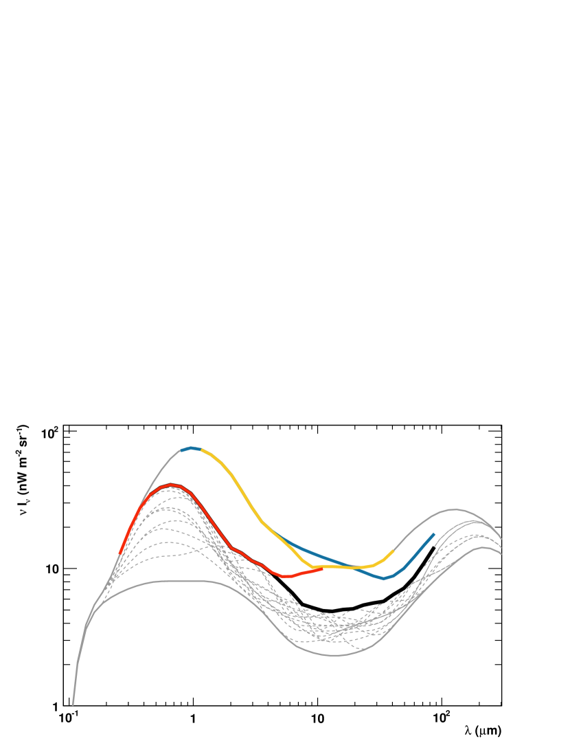
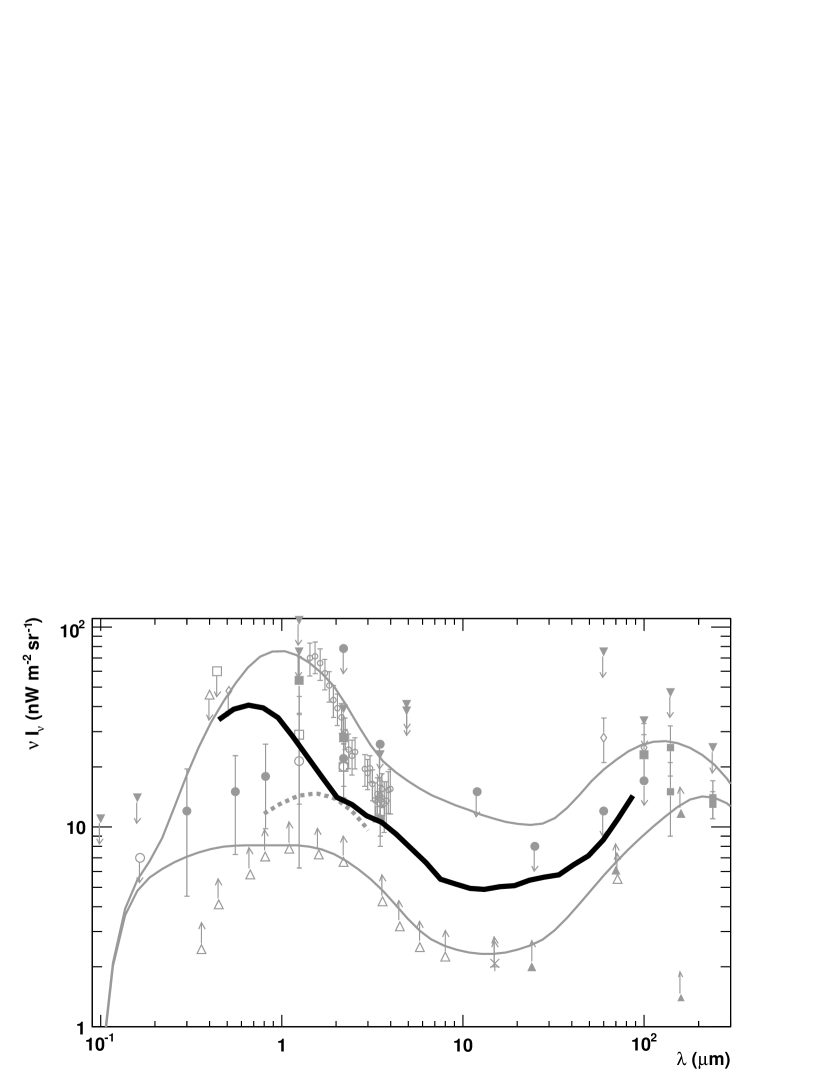
Figure 13: Combined results for the realistic scan. Upper Panel: All highest allowed shapes of the combined scan (dashed grey lines) and the corresponding envelope shape (solid black line) in comparison to the limits for individual spectra: Mkn 501 (solid blue line), H 1426+428 (solid yellow line), and 1ES 1101-232 (solid red line). The minimum and maximum shapes of the scan are also shown (grey lines). Lower Panel: The combined limit from the realistic scan (solid black line) in comparison to direct measurements and limits (grey marker). The grey dashed curve around 2$\,\mu$m is the limit derived by Aharonian et al. (2006a).

Figure 14: Combined results from the extreme scan (dashed black line) in comparison to the result from the realistic scan (solid black line). Grey lines are the minimum and the maximum shapes tested in the scan. Grey markers are direct measurements and limits.

The number of excluded shapes for all individual spectra for the realistic scan are summarized in Table 4. One finds that some spectra (namely 1ES 2344+514, Mkn 180, and PKS 2005-489) excluded none of the EBL shapes of the scan. This mainly is a result of the low statistics in the spectra, hence the large errors on the fit parameters. The highest number of excluded shapes and the strongest constraint in the scan result from the previously presented prototype spectra Mkn 501, H 1426+428, and 1ES 1101-232.

We now combine the results from all spectra by excluding all shapes of the scan, which are excluded by at least one of the spectra. First we present results for the realistic scan. A large fraction of the shapes (98.08%) are excluded by more than one spectra (see Fig. 12), which strengthens our results. In total, we exclude 8 056 718 shapes, which leaves us with only 7 282 (0.01%) allowed shapes. The resulting maximum shapes (dashed lines) and the envelope shape for the combined results are shown in the upper panel of Fig. 13 in comparison to the results from the individual prototype spectra. In the optical-to-near-infrared the combined limit follows exactly the limit derived from the 1ES 1101-232 spectrum. For longer wavelengths, however, the combined limit lies significantly below the limits derived from individual spectra. This is particularly striking in the MIR, where the H 1426+428 spectrum provided only weak limits and the combined limit now gives considerable constraints. This can be understood from the fact that, for a high EBL density in the MIR, a high density in the optical to NIR is needed, so that the spectra (Mkn 501, H 1426+428) will not get too hard. These high densities in the optical-to-NIR are now excluded by the 1ES 1110-232 spectrum, which therefore result in stronger constraints in the MIR.

The combined limit for the realistic scan in comparison to the direct measurements and limits is shown in the lower panel of Fig. 13. In the optical-to-NIR one finds that the combined limit lies significantly below the claimed NIR excess by Matsumoto et al. (2005). It is compatible with the detections reported by Dwek & Arendt (1998), Gorjian et al. (2000), Wright & Reese (2000), and Cambrésy et al. (2001). In the same figure the limit reported by the H.E.S.S. collaboration for 1ES 1101-232 derived with a different technique (Aharonian et al. 2006a) is shown and at wavelengths around 2 - 3$\,\mu$m it is in good agreement with the limit derived here; but for shorter wavelengths our limit lies significantly higher. While for the H.E.S.S. limit comparable exclusion criteria for the spectra were used, a fixed reference shape scaled in the level of the EBL density was used to calculate the EBL limit, which presumably causes the differences at smaller wavelengths. In the MIR to FIR our combined limit lies below all previously reported upper limits from direct measurements and fluctuation analysis. For EBL wavelengths greater than 2$\,\mu$m, it is only about a factor of 2 to 2.5 higher than the absolute lower limit from source counts, leaving very little room for additional contributions to the EBL in this wavelength region. In the FIR it lies more than a factor of $\sim 2$ below the claimed detection by Finkbeiner et al. (2000).

In the realistic scan, after combining the results from Mkn 501, H 1426+428, and 1ES 1110-232, adding more spectra does not further strengthen the limit (though marginal more shapes are excluded). Hence, for the extreme scan, we only combine the results from these three spectra. The limit for the extreme scan is shown in Fig. 14 in comparison to the limit from the realisistic scan. The limit from the extreme scan lies for all EBL wavelengths above the limits from the realistic scan and is a factor of 2.5 to 3.5 higher than the lower limits from source counts. In the optical-to-NIR the combined limit again follows the limit derived from the 1ES 1101-232 spectrum. As stated for the individual spectrum the NIR excess claimed by Matsumoto et al. (2005) for wavelengths above 2$\,\mu$m is now compatible with the limit, but for shorter wavelengths it is still clearly excluded.

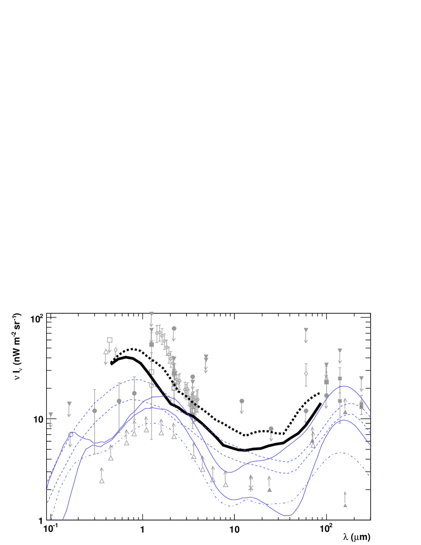
Figure 15: EBL limits from the realistic (thick solid black curve) and the extreme scan (thick dashed black curve) in comparison to different EBL models at $z=0$ (blue curves): updated version of the Kneiske et al. (2002) high and low models (solid), Stecker et al. (2006) fast and baseline evolution models (dashed), Primack et al. (2005) (dashed dotted).

In Fig. 15 the limits derived in this paper are shown in comparison to predictions from EBL models by Kneiske et al. (2002), Stecker et al. (2006), and Primack et al. (2005) (at $z=0$). Most models lie below our realisitc limits. Only the high model of Kneiske et al. (2002) is slightly higher in the NIR, and the fast evolution model of Stecker et al. (2006) is marginally higher in the MIR. These two models are also excluded when applying the criteria from Sect. 4, while the other models are allowed. Noteworthy is that the Primack et al. (2005) and the low model from Kneiske et al. (2002) are below the lower limits derived from galaxy counts in the MIR and FIR.

7 Summary and conclusions

In this paper we present a new method of constraining the density of the extragalactic background light (EBL) in the optical-to-far-infrared wavelength regime using VHE spectra of TeV blazars. We derive strong upper limits, which are only a factor 2 to 3 higher than the lower limits determined from source counts. Unlike what has been done in many previous studies of this kind, we do not use one or a few pre-defined EBL shapes or models, but rather a scan on a grid in EBL density vs. wavelength. This grid covers wavelengths from 0.1 $\mu$m to 1000 $\mu$m and spans in EBL density from the lower limits from source counts to the upper limits determined from direct measurements and fluctuation analyses. By iterating over all scan points, we test a large set of different EBL shapes (8 064 000 in total). Each EBL shape is described by a spline function, which allows us to calculate the optical depth of VHE $\gamma$-rays for this shape via a simple summation instead of solving three integrals numerically. The resolution of the scan for sharp bumps or dips in the EBL is limited by the choice of the grid and the order of the spline.

To test these EBL shapes, we use the measured VHE $\gamma$-ray spectra from distant sources, which carry an imprint of the EBL from attenuation via pair production. We included spectra from all known TeV blazars (13 in total), making this the most complete study of this type up to now. All spectra are scrutinized with the same robust algorithm. For each spectrum and each EBL shape, the intrinsic spectrum is calculated and an analytical description of the intrinsic spectrum is determined by fitting several functions. The fit parameters and errors of the functions are subsequently used to evaluate whether the intrinsic spectrum is physically feasible. We use two conservative criteria from the theory of VHE $\gamma$-ray emission in TeV blazars. The EBL shape is excluded if (i) a part of the intrinsic spectrum is harder than a theoretical limit or (ii) the intrinsic spectrum shows a significant pile-up at high energies. Since there is some spread in the predictions from theory, we included two independent scans for two theoretical limits on the hardness of the spectrum: (1) the realistic case for a photon index of $\Gamma>1.5$ and (2) the extreme case with $\Gamma>2/3$.

We present limits derived from individual VHE $\gamma$-ray spectra. The strongest constraints result from the 1ES 1101-232 spectrum in the wavelength range from 0.8 and 10 $\mu$m, mainly due to the hard spectrum and its large distance to earth. An extragalactic origin of the claimed excess in the NIR between 1 and 2$\,\mu$m (Matsumoto et al. 2005) can be excluded even by the extreme scan. This result confirms the results from the recent publication of Aharonian et al. (2006a). In the FIR (20 and 80 $\mu$m), strong upper limits are provided by the nearby TeV blazar Mkn 501. H 1426+428, situated at an intermediate distance, provides some constraints on the EBL density in the MIR (between 1 and 15 $\mu$m), connecting the upper limits derived from 1ES 1101-232 and Mkn 501. Most of the other spectra provide constraints in certain wavelength ranges, but they are not as strong as the limits from the previously described sources.

By combining the results from all spectra, we find that the upper limits become much stronger compared to the limits derived for individual spectra, especially in the wavelength range between 4 and 60 $\mu$m. In the wavelength region from 2 to 80$\,\mu$m, the combined limit for the realistic case lies below the upper limits derived from fluctuation analyses of the direct measurements (Kashlinsky & Odenwald 2000) and is just a factor of 2 to 2.5 above the absolute lower limits from source counts. This makes it the most constraining limit in the MIR to FIR region so far. As expected, the upper limits from the extreme scan are less constraining (factor of 2.5 to 3.5 above the lower limit from source counts), but still substantial over this wide wavelength range.

The derived upper limits can be interpreted in two different ways:

1. The EBL density in the optical-to-FIR is significantly lower than suggested by direct measurements, and the actual EBL level seems to be close to the existing lower limits. It can thus be concluded that experiments like HST, ISO, and Spitzer resolve most of the sources in the universe. This would indicate that there is very little room left for a significant contribution of heavy and bright Population III stars to the EBL density in this wavelength region.

2. The assumptions used for this study are not correct. This would require a revision of the current understanding of TeV blazar physics and models, which has so far been fairly successful in modeling multi-wavelength data from the radio to the VHE for all detected sources.

We estimate that the main contribution to the systematic errors arises from the minimum width of the EBL structures that can be resolved by the scan. Although the choice of the grid spacing, which defines the minimum width of the EBL structures, is physically well motivated, there are arguments that even thinner structures could be realized in nature due to, say absorption effects. We tested a 20% smaller grid spacing, resulting in much less realistic, but still possible, EBL structures, with the 1ES 1101-232 spectrum. The resulting limits on the EBL are 20 to 30% higher than the ones presented in Section 5.3. We therefore conclude that the overall contribution from the grid setup to the systematic error is at most 30%.

Another contribution to the systematic error originates from not considering the evolution of the EBL in our method. To estimate the effect of the evolution of the EBL for the most distant sources, we calculate the late contribution to the EBL in the redshift interval between $z=0$ and $z=0.2$. Here, we utilize the EBL model by Kneiske et al. (2002) (updated version is used, Kneiske private communication). We obtain a wavelength dependent contribution, which has a maximum value of 3-4 nW m^-2sr^-1 in the optical to NIR (the relevant wavelength region for the distant sources in our scan). Given that these values are derived with the extreme assumption that all late emission occured instantaneously at z=0, we estimate the systematic error arising from the EBL evolution to 10% of the derived limits. Note that Aharonian et al. (2006a) estimated an error of $<$10% for the most distant TeV blazar in our study 1ES 1101-232.

To study the effect of the uncertainties in the absolute energy scale of IACT measurements, we calculate a limit on the EBL utilizing the energy spectra from Mkn 501, H 1426+428, and 1ES 1101-232 shifted by 15% to lower energies (for $\Gamma>1.5$, realistic scan). Since the optical depth is increasing with energy, the energy shift reduces the attenuation of the spectra, especially reducing the effect of a possible pile-up at the highest energies. The difference between the limit derived from the energy shifted spectra and the realistic limit is negligible in the optical to NIR ($<$6 $\mu$m), while there is a moderate effect in the MIR to FIR on the level of 1 – 4.5 nW m^-2sr^-1. We therefore conclude that the systematic error in the MIR to FIR ($\lambda>6\,\mu$m) introduced by the uncertainties in the absolute energy scale of IACT measurements is close to 10–45% of our realistic limit.

Adding the individual errors quadratically, we finally conclude that the (very conservative) systematic error on the upper limit is about 32% in the optical-to-NIR and 33 – 55% in MIR to FIR.

The strong constraints derived in this paper only allow for a low level of the EBL in the optical to the far-infrared, suggesting that the universe is more transparent to VHE $\gamma$-rays than previously thought. Hence, we expect detections of many new extragalactic VHE sources in the next few years. Further multi-wavelength studies of TeV blazars will improve the understanding of the underlying physics, which will help to refine the exclusion criteria for the VHE spectra in this kind of study. The upcoming GLAST satellite experiment, operating in an energy range from 0.1 up to $\sim$100 GeV, will allow such studies of the EBL to be extended to the ultraviolet-to-optical wavelength region. A detailed analysis of the impact of our constraints on the contribution from Population III stars to the EBL is in preparation.

Appendix A Likelihood Ratio Test

The likelihood ratio test (Eadie et al. 1988) is a standard statistical tool to test between two hypotheses whether an improvement to a fit quality (quantified by corresponding $\chi^{2}$ values) is expected from a normal distribution or if it is significant. By fitting two functional forms to the intrinsic spectrum, one obtains values of the likelihood functions $L_{A}$ and $L_{B}$. If hypothesis A is true, the likelihood ratio $R=-\ln(L_{A}/L_{B})$ is approximately $\chi^{2}$ distributed with $N$ degrees of freedom. $N$ is the difference between numbers of degrees of freedom of hypothesis A and hypothesis B. One defines a probability

$$P=\int\limits_{0}^{R_{\mathrm{meas}}}p\,(\chi^{2})\,\mathrm{d\chi^{2}}$$ (9)

where $p\,(\chi^{2})$ is the $\chi^{2}$ probability density function and $R_{meas}$ the measured value of $R$. Hypothesis A will be rejected (and hypothesis B will be accepted) if $P$ is greater than the confidence level, which is set to 95%.

References

- Aharonian et al. (2005a) Aharonian, F., Akhperjanian, A. G., Aye, K.-M., et al. 2005a, A&A, 436, L17
- Aharonian et al. (2005b) Aharonian, F., Akhperjanian, A. G., Bazer-Bachi, A. R., et al. 2005b, A&A, 442, 895
- Aharonian et al. (2006a) Aharonian, F., Akhperjanian, A. G., Bazer-Bachi, A. R., et al. 2006a, Nature, 440, 1018
- Aharonian et al. (2006b) Aharonian, F., Akhperjanian, A. G., Bazer-Bachi, A. R., et al. 2006b, A&A, 455, 461
- Aharonian et al. (2006c) Aharonian, F., Akhperjanian, A. G., Bazer-Bachi, A. R., et al. 2006c, A&A, 448, L19
- Aharonian et al. (2006d) Aharonian, F., Akhperjanian, A. G., Bazer-Bachi, A. R., et al. 2006d, Science, 314, 1424
- Aharonian (2001) Aharonian, F. A. 2001, in Proceedings of 27th ICRC, Highlight papers, Hamburg, ed. R. Schlickeiser, 250
- Aharonian et al. (2002a) Aharonian, F. A., Akhperjanian, A., Beilicke, M., et al. 2002a, Astronomy and Astrophysics, 393, 89
- Aharonian et al. (1999) Aharonian, F. A., Akhperjanian, A. G., Barrio, J. A., et al. 1999, Astronomy and Astrophysics, 349, 11
- Aharonian et al. (2002b) Aharonian, F. A., Akhperjanian, A. G., Barrio, J. A., et al. 2002b, Astronomy and Astrophysics, 384, L23
- Aharonian et al. (2003a) Aharonian, F. A., Akhperjanian, A. G., Beilicke, M., et al. 2003a, Astronomy and Astrophysics, 406, L9
- Aharonian et al. (2003b) Aharonian, F. A., Akhperjanian, A. G., Beilicke, M., et al. 2003b, Astronomy and Astrophysics, 403, L1
- Aharonian et al. (2003c) Aharonian, F. A., Akhperjanian, A. G., Beilicke, M., et al. 2003c, Astronomy and Astrophysics, 403, 523, astro-ph/0301437
- Aharonian et al. (2002c) Aharonian, F. A., Timokhin, A. N., & Plyasheshnikov, A. V. 2002c, A&A, 384, 834
- Albert et al. (2006a) Albert, J., Aliu, E., Anderhub, H., et al. 2006a, ApJ, 642, L119
- Albert et al. (2006b) Albert, J., Aliu, E., Anderhub, H., et al. 2006b, ApJ, 648, L105
- Albert et al. (2007a) Albert, J., Aliu, E., Anderhub, H., et al. 2007a, ApJ, 654, L119
- Albert et al. (2007b) Albert, J., Aliu, E., Anderhub, H., et al. 2007b, ApJ, 663, 125
- Bernstein et al. (2002) Bernstein, R. A., Freedman, W. L., & Madore, B. F. 2002, Astrononmy and Astrophysics, 571, 56
- Bernstein et al. (2005) Bernstein, R. A., Freedman, W. L., & Madore, B. F. 2005, ApJ, 632, 713
- Brown et al. (2000) Brown, T. M., Kimble, R. A., Ferguson, H. C., et al. 2000, AJ, 120, 1153
- Cambrésy et al. (2001) Cambrésy, L., Reach, W. T., Beichman, C. A., & Jarrett, T. H. 2001, The Astrophysical Journal, 555, 563
- Cortina et al. (2005) Cortina, J. et al. 2005, in International Cosmic Ray Conference, Vol. 5, 359
- Costamante et al. (2003) Costamante, L., Aharonian, F., Ghisellini, G., & Horns, D. 2003, New Astronomy Review, 47, 677
- Daum et al. (1997) Daum, A., Hermann, G., Hess, M., et al. 1997, Astroparticle Physics, 8, 1
- Dole et al. (2006) Dole, H., Lagache, G., Puget, J.-L., et al. 2006, A&A, 451, 417
- Dube et al. (1979) Dube, R. R., Wickes, W. C., & Wilkinson, D. T. 1979, ApJ, 232, 333
- Dwek & Arendt (1998) Dwek, E. & Arendt, R. G. 1998, The Astrophysical Journal, 508, L9
- Dwek et al. (2005a) Dwek, E., Arendt, R. G., & Krennrich, F. 2005a, ApJ, 635, 784
- Dwek & Krennrich (2005) Dwek, E. & Krennrich, F. 2005, ApJ, 618, 657
- Dwek et al. (2005b) Dwek, E., Krennrich, F., & Arendt, R. G. 2005b, ApJ, 634, 155
- Dwek & Slavin (1994) Dwek, E. & Slavin, J. 1994, ApJ, 436, 696
- Eadie et al. (1988) Eadie, W. T., Drijard, D., James, F. E., Roos, M., & Sadoulet, B. 1988, Statistical Methods in Experimental Physics (North-Holland Publishing Company; Amsterdam, New-York, Oxford)
- Edelstein et al. (2000) Edelstein, J., Bowyer, S., & Lampton, M. 2000, ApJ, 539, 187
- Elbaz et al. (2002) Elbaz, D., Cesarsky, C. J., Chanial, P., et al. 2002, Astronomy and Astrophysics, 384, 848
- Fazio et al. (2004) Fazio, G. G., Ashby, M. L. N., Barmby, P., et al. 2004, ApJS, 154, 39
- Fazio & Stecker (1970) Fazio, G. G. & Stecker, F. W. 1970, Nature, 226, 135
- Finkbeiner et al. (2000) Finkbeiner, D. P., Davis, M., & Schlegel, D. J. 2000, The Astrophysical Journal, 544, 81
- Finley & The VERITAS Collaboration (2001) Finley, J. P. & The VERITAS Collaboration. 2001, in International Cosmic Ray Conference, 2827–+
- Frayer et al. (2006) Frayer, D. T., Huynh, M. T., Chary, R., et al. 2006, ApJ, 647, L9
- Gaidos et al. (1996) Gaidos, J. A., Akerlof, C. W., Biller, S. D., et al. 1996, Nature, 383, 319
- Gorjian et al. (2000) Gorjian, V., Wright, E. L., & Chary, R. R. 2000, The Astrophysical Journal, 536, 550
- Gould & Schréder (1967) Gould, R. J. & Schréder, G. P. 1967, Physical Review, 155, 1408
- Guy et al. (2000) Guy, J., Renault, C., Aharonian, F. A., Rivoal, M., & Tavernet, J.-P. 2000, Astronomy and Astrophysics, 359, 419
- Hauser et al. (1998) Hauser, M. G., Arendt, R. G., Kelsall, T., et al. 1998, The Astrophysical Journal, 508, 25
- Hauser & Dwek (2001) Hauser, M. G. & Dwek, E. 2001, Annual Review of Astronomy and Astrophysics, 39, 249
- Heitler (1960) Heitler, M. 1960, The Quantum Theorie of Radiation (Oxford, Clarendon)
- Hinton (2004) Hinton, J. A. 2004, New Astronomy Review, 48, 331
- Horan & Weekes (2004) Horan, D. & Weekes, T. C. 2004, New Astronomy Review, 48, 527
- Kashlinsky (2005) Kashlinsky, A. 2005, Phys. Rep, 409, 361
- Kashlinsky et al. (2005) Kashlinsky, A., Arendt, R. G., Mather, J., & Moseley, S. H. 2005, Nature, 438, 45
- Kashlinsky et al. (1996) Kashlinsky, A., Mather, J., Odenwald, S., & Hauser, M. 1996, The Astrophysical Journal, 470, 681
- Kashlinsky & Odenwald (2000) Kashlinsky, A. & Odenwald, S. 2000, The Astrophysical Journal, 528, 74
- Katarzyński et al. (2006) Katarzyński, K., Ghisellini, G., Tavecchio, F., Gracia, J., & Maraschi, L. 2006, MNRAS, 368, L52
- Kifune (1999) Kifune, T. 1999, ApJ, 518, L21
- Kneiske et al. (2004) Kneiske, T. M., Bretz, T., Mannheim, K., & Hartmann, D. H. 2004, A&A, 413, 807
- Kneiske et al. (2002) Kneiske, T. M., Mannheim, K., & Hartmann, D. H. 2002, A&A, 386, 1
- Krennrich et al. (2002) Krennrich, F., Bond, I. H., Bradbury, S. M., et al. 2002, ApJ, 575, L9
- Lagache & Puget (2000) Lagache, G. & Puget, J.-L. 2000, Astronomy and Astrophysics, 355, 17
- Leinert et al. (1998) Leinert, C., Bowyer, S., Haikala, L. K., et al. 1998, A&AS, 127, 1
- Levenson et al. (2007) Levenson, L. R., Wright, E. L., & Johnson, B. D. 2007, ArXiv e-prints, 704
- Madau & Pozzetti (2000) Madau, P. & Pozzetti, L. 2000, Monthly Notices of the Royal Astronomical Society, 312, L9
- Mapelli et al. (2004) Mapelli, M., Salvaterra, R., & Ferrara, A. 2004, in Baryons in Dark Matter Halos, ed. R. Dettmar, U. Klein, & P. Salucci
- Martin et al. (1991) Martin, C., Hurwitz, M., & Bowyer, S. 1991, ApJ, 379, 549
- Matsumoto et al. (2005) Matsumoto, T., Matsuura, S., Murakami, H., et al. 2005, ApJ, 626, 31
- Mattila (1990) Mattila, K. 1990, in IAU Symp. 139: The Galactic and Extragalactic Background Radiation, ed. S. Bowyer & C. Leinert, 257–268
- Matute et al. (2006) Matute, I., La Franca, F., Pozzi, F., et al. 2006, A&A, 451, 443
- Metcalfe et al. (2003) Metcalfe, L., Kneib, J.-P., McBreen, B., et al. 2003, A&A, 407, 791
- Papovich et al. (2004) Papovich, C., Dole, H., Egami, E., et al. 2004, ApJS, 154, 70
- Primack et al. (1999) Primack, J., Bullock, J., Summerville, R., & MacMinn, D. 1999, Astroparticle Physics, 11, 93
- Primack et al. (2005) Primack, J. R., Bullock, J. S., & Somerville, R. S. 2005, in AIP Conf. Proc. 745: High Energy Gamma-Ray Astronomy, ed. F. A. Aharonian, H. J. Völk, & D. Horns, 23–33
- Protheroe & Meyer (2000) Protheroe, R. J. & Meyer, H. 2000, Physics Letters B, 493, 1
- Punch et al. (1992) Punch, M., Akerlof, C. W., Cawley, M. F., et al. 1992, Nature, 358, 477
- Salvaterra & Ferrara (2003) Salvaterra, R. & Ferrara, A. 2003, Monthly Notice of the Royal Astronomical Society, 339, 973
- Salvaterra & Ferrara (2006) Salvaterra, R. & Ferrara, A. 2006, MNRAS, 367, L11
- Schroedter et al. (2005) Schroedter, M., Badran, H. M., Buckley, J. H., et al. 2005, ApJ, 634, 947
- Stecker et al. (1996) Stecker, F. W., de Jager, O. C., & Salamon, M. H. 1996, ApJ, 473, L75+
- Stecker & Glashow (2001) Stecker, F. W. & Glashow, S. L. 2001, Astroparticle Physics, 16, 97
- Stecker et al. (2006) Stecker, F. W., Malkan, M. A., & Scully, S. T. 2006, ApJ, 648, 774
- Toller (1983) Toller, G. N. 1983, ApJ, 266, L79
- Wright & Reese (2000) Wright, E. L. & Reese, E. D. 2000, The Astrophysical Journal, 545, 43