Sustained Magneto-Shear Instabilities in the Solar Tachocline

Abstract

We present nonlinear three-dimensional simulations of the stably-stratified portion of the solar tachocline in which the rotational shear is maintained by mechanical forcing. When a broad toroidal field profile is specified as an initial condition, a clam-shell instability ensues which is similar to the freely-evolving cases studied previously. After the initial nonlinear saturation, the residual mean fields are apparently too weak to sustain the instability indefinitely. However, when a mean poloidal field is imposed in addition to the rotational shear, a statistically-steady state is achieved in which the clam-shell instability is operating continually. This state is characterized by a quasi-periodic exchange of energy between the mean toroidal field and the instability mode with a longitudinal wavenumber $m=1$. This quasi-periodic behavior has a timescale of several years and may have implications for tachocline dynamics and field emergence patterns throughout the solar activity cycle.

1. Introduction

It is now well established (at least from a theoretical perspective) that axisymmetric rings of toroidal field in the solar tachocline are susceptible to global instabilities induced by the latitudinal differential rotation. This was first demonstrated for 2–D spherical surfaces (Gilman & Fox, 1997, 1999; Dikpati & Gilman, 1999; Gilman & Dikpati, 2000; Cally et al., 2003; Dikpati et al., 2004a) and was later extended to 3–D spherical shells under the shallow-water approximation (Gilman & Dikpati, 2002; Dikpati et al., 2003) and the thin-shell approximation (Cally, 2003; Miesch et al., 2007; Gilman et al., 2007). For strong fields (such that the magnetic energy is comparable to the kinetic energy contained in the differential rotation), the most unstable modes have longitudinal wavenumber $m=1$, which corresponds to a tipping of the ring such that its central axis becomes misaligned with the rotation axis.

This class of global magneto-shear instabilities occurs both for concentrated bands of toroidal field and for broad field profiles. The preferred mode for broad field profiles which are antisymmetric about the equator is the clam-shell instability whereby toroidal rings in the northern and southern hemispheres tip out of phase, reconnecting at the equator on one side of the sphere and opening up on the other side (Cally, 2001; Cally et al., 2003; Miesch et al., 2007). In the absence of external forcing, the instability proceeds until loops of field become perpendicular to the equatorial plane and the latitudinal shear is nearly eliminated.

However, the solar tachocline is not an isolated system. Rotational shear is continually maintained by stresses from the overlying convection zone and the underlying radiative interior. Meanwhile, magnetic flux is continually being replenished from above by penetrative convection and meridional circulation. If clam-shell instabilities are indeed occurring in the tachocline, their environment is likely much more dynamic than the freely-evolving scenarios considered in previous nonlinear simulations (Cally, 2001; Cally et al., 2003; Miesch et al., 2007).

In this letter we present the first nonlinear simulations of global magneto-shear instabilities in the solar tachocline in which the instabilities are continually maintained against nonlinear saturation and dissipation through the use of external forcing. We use the same nonlinear, 3–D thin-shell model employed by Miesch et al. (2007, hereafter MGD07) to study the freely-evolving case. The linear stability of this thin-shell system has been investigated by Gilman et al. (2007). The reader is referred to these two papers for a much more comprehensive discussion of the unstable modes and their nonlinear saturation under freely-evolving conditions. These papers also contain a more comprehensive discussion of related work and a more detailed description of the thin-shell model and the numerical algorithm.

The first question we address in this letter is whether the instabilities can generate poloidal fields efficiently enough to act as a dynamo when only mechanical forcing of the rotational shear is applied. Our simulations suggest that this is unlikely although the results are inconclusive. However, statistically steady states are found when the magnetic energy is maintained via a poloidal forcing term in the mean induction equation. These states exhibit a quasi-periodic behavoir as mean fields continually transfer energy to the non-axisymmetric instability modes and are then re-established by the mechanical and magnetic forcing.

2. The Thin-Shell Model

Our numerical model is based on the thin-shell approximation which is described in detail by Miesch & Gilman (2004) and MGD07. The aspect ratio $\delta=D/R$ is assumed to be much less than unity, where $D$ and $R$ are the width and radial location of the computational domain. Only terms of lowest order in $\delta$ are retained in the equations of motion and the layer is assumed to be stably-stratified, corresponding to the lower portion of the solar tachocline (Thompson et al., 2003). The equations are expressed in a rotating, spherical polar coordinate system defined by the colatitude $\theta$, longitude $\phi$ and height $z$ with corresponding unit vectors $\hat{\theta}$, $\hat{\phi}$, and $\hat{z}$. The velocity and magnetic field components are defined as ${\bf v}=u\mbox{\boldmath$\hat{\phi}$}+v\mbox{\boldmath$\hat{\theta}$}+\delta w\mbox{\boldmath$\hat{z}$}$ and $\mbox{\boldmath$B$}=a\mbox{\boldmath$\hat{\phi}$}+b\mbox{\boldmath$\hat{\theta}$}+\delta c\mbox{\boldmath$\hat{z}$}$. The system is made nondimensional through the use of horizontal and vertical length scales $R$ and $D$, a velocity scale based on the equatorial rotation rate, and the background density and entropy gradient. We neglect pressure variations relative to entropy variations in the linearized equation of state which corresponds to the Boussinesq limit discussed by MGD07 [$\delta_{P}=0$ in their equation (6)]. Apart from the parameters which specify the forcing, dissipation, and initial conditions, this leaves one free parameter: the Froude number $F_{r}$, which is a nondimensional measure of the stratification. For the simulations discussed here we take $F_{r}=0.1$ as appropriate for the lower tachocline (MGD07).

The subgrid-scale (SGS) model consists of a fourth-order hyperdiffusion in the horizontal dimensions with an effective Reynolds number of $R_{h}$ and a Smagorinsky formulation for the vertical diffusion involving a vertical Reynolds number $R_{v}$ (MGD07). The amplitude and form of the SGS magnetic and thermal diffusion are assumed to be the same as the viscous diffusion, implying magnetic and thermal Prandtl numbers of unity. The upper and lower boundaries of the layer are assumed to be impenetrable, stress-free, perfectly conducting, and isentropic.

Mechanical forcing is imposed by adding a volumetric source term to the momentum equation of the form

$$\mbox{\boldmath$F$}_{u}(\theta,z)=\tau^{-1}\left(u_{0}-\left<u\right>\right)\mbox{\boldmath$\hat{\phi}$}$$ (1)

where $u$ is the zonal velocity, $\tau$ is a characteristic timescale for the establishment of the shear and

$$u_{0}(\theta,z)=\frac{1}{2}\left(1-\cos\left(\pi z\right)\right)\left(s_{0}-s_{2}\cos^{2}\theta\right)\sin\theta~{}~{}~{}.$$ (2)

Angular brackets $<>$ in equation (1) denote an average over longitude. In equation (2), $s_{0}$ is the nondimensional equatorial rotation rate relative to the rotating reference frame and $s_{2}$ is the fractional angular velocity difference between the equator and poles. Here we take $s_{0}=0.044$ and $s_{2}=0.18$ (MGD07). The vertical profile of $u_{0}$ is such that the latitudinal shear is maximum at the top of the layer ($z=1$) and vanishes at the bottom ($z=0$) in analogy with the solar tachocline.

In selected cases we also impose a dipolar field by means of a similar forcing term added to the induction equation:

$$\mbox{\boldmath$F$}_{p}(\theta,z)=\tau^{-1}\left(\mbox{\boldmath$B$}_{0}-\left<\mbox{\boldmath$B$}_{p}\right>\right)$$ (3)

where $\mbox{\boldmath$B$}_{p}=b\mbox{\boldmath$\hat{\theta}$}+\delta c\mbox{\boldmath$\hat{z}$}$ and

$$\mbox{\boldmath$B$}_{0}(\theta,z)=\mbox{\boldmath$\nabla\times$}\mbox{\boldmath$\nabla\times$}\left[C_{0}\cos\theta\sin(\pi z)\mbox{\boldmath$\hat{z}$}\right]~{}~{}~{}.$$ (4)

This field is intented to represent generated by dynamo processes in the convection zone and pumped downward. Imposing $\mbox{\boldmath$B$}_{0}$ together with $u_{0}$ is an indirect way of imposing a mean toroidal field; the latitudinal shear in the upper portion of the layer stretches and amplifies the poloidal field through what is known as the $\Omega$-effect, resulting in a mean toroidal field $\left<a\right>$ which is antisymmetric about the equator. The peak amplitude of $\left<a\right>$ will in general depend on the poloidal field strength $C_{0}$, on the SGS diffusion, and to some extent on $F_{r}$.

Figure 1.— The volume-integrated magnetic energy contained in the mean toroidal field (TFME, solid line), the mean poloidal field (PFME, dash-dotted line) and the non-axisymmetric field (NAME, dotted line) are shown as a function of time in a simulation with no magnetic forcing ($R_{h}=10^{7}$, $R_{v}=10^{4}$, $\tau=0.1$). All curves are normalized relative to the integrated kinetic energy contained in the imposed shear profile $u_{0}$ (indicated by the horizontal dashed line).

Figure 2.— As in Figure 1 for a case with both mechanical and magnetic forcing as described in the text ($R_{h}=10^{5}$, $R_{v}=10^{4}$, $\tau=0.1$). Note that the vertical axis is linear here rather than logarithmic. Vertical dashed lines indicate the time instances illustrated in Figure 3.

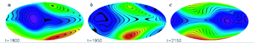
Figure 3.— The horizontal structure of the magnetic potential $J$ near the top of the layer ($z=0.98$) is illustrated at three different times for the same simulation as shown in Figure 2. The color table varies with increasing $J$ as blue-green-yellow-red. Black countours trace horizontal magnetic field lines as noted in the text, although the sense of the field is opposite in the northern and southern hemispheres. Each horizontal surface is displayed as a Molleweide projection in which lines of constant latitude appear horizontal.

3. Sustained Magneto-Shear Instabilities

Our simulations are initiated as described in MGD07, with an equilibrium state defined by the zonal velocity $u_{0}$ and a broad toroidal field profile of the form

$$a(\theta)=\alpha\cos\theta\sin\theta~{}~{}~{}.$$ (5)

The initial pressure and temperature are chosen such that the initial state is in magneto-hydrostatic and magneto-geostrophic balance. The parameter $\alpha$ is set to unity for the simulations presented here, corresponding to a peak dimensional field strength of about 40 kG, toward the high end of the range expected to exist in the tachocline (MGD07). Global magneto-shear instabilities also occur for weaker fields but they take longer to develop. The initial equilibrium state is perturbed by adding a random, small-scale velocity field.

Unlike the simulations presented in MGD07, we maintain the differential rotation through the forcing term defined in equation (1). An example of the subsequent evolution in the absence of magnetic forcing ($\mbox{\boldmath$F$}_{p}={\bf 0}$) is shown in Figure 1. The spatial resolution used for this case is $N_{\theta}$, $N_{\phi}$, $N_{z}$ = 128, 256, 210.

Figure 1 shows the components of the magnetic energy integrated over the volume of the shell. One time unit in the nondimensional system corresponds to about four days (MGD07). At early times the mean toroidal field (TFME) dominates but the non-axisymmetric component (NAME) grows rapidly as the clam-shell instability develops. Most of the NAME is in the $m=1$ mode which dominates the total magnetic energy after the instability saturates at $t\sim 400$.

The evolution shown in Figure 1 is very similar to the unforced cases discussed at length in MGD07. However, in the absence of mechanical forcing, the saturation of the clam-shell instability induces a global redistribution of angular momentum which reverses the sense of the differential rotation (MGD07). The forcing suppresses this, leaving the differential rotation profile unchanged after saturation.

After saturation, the magnetic energy in the mean toroidal field decreases as in the unforced case, despite the persistent rotational shear. The TFME oscillates with a period of about 15 time units, corresponding to about two months. At later times, the amplitude of the oscillation decreases and the period increases slightly, to about 18 time units. This oscillation appears to be induced by a standing Alfvén wave excited by the initial saturation of the instability. However, low-wavenumber Rossby waves are also excited and have a comparable period.

In shallow-water systems which have a deformable upper boundary, global magneto-shear instabilities can possess significant kinetic helicity, suggesting they may serve to generate poloidal field from toroidal field and thus drive a self-sustained dynamo contained entirely within the tachocline (Dikpati & Gilman, 2001a; Gilman & Dikpati, 2002; Dikpati et al., 2003).

The simulation shown in Figure 1 does not extend more than a diffusive timescale ($\sim 10^{5}$ time units) so it is uncertain whether or not it may be classified as a dynamo. The energy in the mean fields may be levelling off beyond $t\sim 800$ but it is unclear whether this state will persist indefinitely. A more diffusive analogue of this case ($R_{h}=10^{5}$) was certainly not a dynamo since the total magnetic energy decayed steadily after the initial saturation.

In any case, it appears either that the clam-shell instability is no longer operating beyond $t\sim 500$ or that it is operating on a much longer time scale. The magnetic energy remains dominated by the $m=1$ component for at least five years in dimensional time units. Over this time period the energy in the mean toroidal field remains larger than the equipartition energy associated with the imposed differential rotation but the energy in the mean poloidal field is about three orders of magnitude smaller. These fields appear to be a remnant of the initial saturation of the instability at $t\sim 400$ as opposed to dynamo-generated fields induced by ongoing instabilities.

The situation changes dramatically if a mean poloidal field is imposed through the forcing term expressed in equation (3). Figure 2 illustrates the evolution of the magnetic energy components in a simulation with both mechanical and magnetic forcing ($N_{\theta}=64$, $N_{\phi}=128$, $N_{z}=210$). The time span shown covers a period beyond the initial saturation of the instability, after a statistically steady state has been reached.

The time evolution shown in Figure 2 reflects a quasi-periodic exchange of energy between the mean toroidal field and the non-axisymetric field components, the latter dominated by the $m=1$ mode. The first two oscillations shown each span about 340 time units which corresponds to 3.7 years. However, the TFME drops lower in the subsequent cycle, reaching a minimum at $t\sim 1950$, leading to a longer cycle of about 400 time units (4.4 years). The following cycle is then much shorter, lasting only about 230 time units (2.5 years). The shape of each cycle is asymmetric, with a relatively slow rise in TFME followed by a sharper drop as the clam-shell instability sets in.

The non-axisymmetric magnetic energy exhibits quasi-periodic cycles similar to the mean toroidal field but phase-shifted such that the maxima in NAME occur as the TFME is decreasing. Again, this reflects the repeated development of the clam-shell instability which transfers energy from the mean toroidal field to the $m=1$ components. After the instability saturates, the mechanical and magnetic forcing re-establish the mean fields and the next cycle proceeds.

To gain further insight into the dynamics, it is instructive to express the magnetic field in terms of scalar magnetic potentials $J$ and $C$ defined such that

$$\mbox{\boldmath$B$}=\mbox{\boldmath$\nabla\times$}\left(J\mbox{\boldmath$\hat{z}$}\right)+\mbox{\boldmath$\nabla\times$}\mbox{\boldmath$\nabla\times$}\left(C\mbox{\boldmath$\hat{z}$}\right)~{}~{}~{}.$$ (6)

In the simulations reported here, as in the freely evolving cases reported in MGD07, the magnetic field remains predominantly horizontal and the first term on the right-hand-side of equation (6) dominates. Thus, to a good approximation, contours of $J$ trace the horizontal field lines as illustrated in Figure 3 [$\mbox{\boldmath$\nabla\times$}(J\mbox{\boldmath$\hat{z}$})=\mbox{\boldmath$\hat{z}$}\mbox{\boldmath$\times$}\mbox{\boldmath$\nabla$}J$].

The changing patterns shown in Figure 3 illustrate the competing effects of the forcing and the instabilities. At $t=1800$ (Fig. 3$a$), the mean toroidal field dominates the magnetic energy, although non-axisymmetric structure is evident. By $t=1950$ the clam-shell instability has transferred much of this energy to the $m=1$ mode and horizontal field lines are oriented more north-south (Fig. 3$b$). The imposed shear then operates on these fields as well as the imposed poloidal field to rebuild the mean toroidal field which again dominates by $t=2150$ (Fig. 3$c$).

The vertical structure of the flow is similar to analogous freely-evolving cases with vertical shear discussed in MGD07. The velocity and magnetic fluctuations remain predominantly horizontal and the instability proceeds most vigorously near the top of the layer where the latitudinal shear is strongest.

For the simulation shown in Figures 2 and 3, the amplitude of the imposed poloidal field, $C_{0}$, is such that the integrated magnetic energy PFME is about twice the equipartion value $u_{0}^{2}/2$ (integrated over the volume). This ratio is somewhat smaller near the top of the layer where the latitudinal shear peaks but nevertheless it is probably unrealistically large for the solar tachocline. Weaker imposed fields could potentially produce mean toroidal fields of comparable strength but this can only be achieved in a simulation if the SGS diffusion is sufficiently low. Indeed, an analogous simulation with a weaker imposed field (PFME/DRKE = 0.02) and the same diffusion coefficients ($R_{h}=10^{5}$, $R_{v}=10^{4}$) produced weaker mean toroidal fields (TFME/DRKE $\sim$ 3). This system also exhibits sustained clam-shell instabilities with quasi-periodic behavior but the phase relationship between the TFME and NAME is not as well defined as in Figure 2. Some quasi-periodic oscillations are present on timescales of several years but longer-term trends are also evident, comparable to or longer than the duration of the simulation ($\sim$ 10 years). Such longer-term evolution is to be expected since the growth rate of the clam-shell instability decreases with decreasing field strength.

Achieving substantially lower SGS diffusion would require higher resolution which is a challenge because of the long integration times necessary to capture multiple cycles. The relatively short forcing timescale used for the simulations shown in Figures 1-3 ($\tau=0.1$, corresponding to about 10 hours) is also in some sense required by the setup of our numerical experiments. In a simulation similar to that shown in Figures 2-3 but with $\tau=2$ (8 days), the mechanical forcing is insufficient to overcome the magnetic tension associated with the imposed poloidal field. As a result, the DRKE is only 20% of the target value associated with $u_{0}$ and the clam-shell instability is suppressed. The field does exhibit $m=1$ structure but TFME dominates the magnetic energy and the evolution is quasi-steady, with a slow retrograde propagation and no episodic opening up of the clam-shell pattern.

The solar tachocline is much more complex than our highly simplified model. Forcing timescales are longer but the diffusion is lower, so strong toroidal fields could be produced with lower poloidal field strengths and the differential rotation could be maintained with weaker mechanical forcing. It is therefore difficult to establish from the simulations alone whether the solar tachocline is in a regime which exhibits quasi-periodic behavoir as in Figure 2. However, helioseismic inversions indicate that the rotational shear in the tachocline is continually maintained and linear analysis suggests that even weak toroidal fields are unstable in the presence of such shear so it is likely that the tachocline is indeed continually undergoing global magneto-shear instabilities.

Latitudinal shear in the convective envelope is maintained by Reynolds stresses and meridional circulations on timescales of order months while the nearly uniform rotation of the radiative interior may be established on much longer time scales (e.g. Gough & McIntyre, 1998; Talon et al., 2002; Miesch, 2005). Magnetic flux is continually supplied to the tachocline by topological pumping from penetrative convection (e.g. Tobias et al., 2001). Although much of this flux is disordered, mean fields may be generated by nonlinear self-organization processes such as inverse cascades or by rotational phase mixing and turbulent reconnection (Spruit, 1999; Browning et al., 2006). In addition, global meridional circulations may transport axisymmetric poloidal flux to the tachocline where mean toroidal fields would then be generated by rotational shear (Dikpati et al., 2004b; Charbonneau, 2005).

In this letter we have demonstrated that the clam-shell instability can operate continually when rotational shear and magnetic fields are continually replenished. The temporal evolution is quasi-periodic and as mean fields alternately build up and destabilize. This has the character of a critical phenomenon but it is not self-organized criticality in the technical sense because there is a characteristic time and spatial scale associated with the growth rate and wavenumber of the instability (Jensen, 1998). It is likely that other instability modes may similarly be maintained continually by external forcing. Notable among these is the $m=1$ tipping instability which exists for the type of concentrated toroidal bands thought to give rise to photospheric active regions (Dikpati & Gilman, 1999; Cally et al., 2003; Miesch et al., 2007).

If global magneto-shear instabilities are indeed occurring in the solar tachocline they would have wide-ranging implications for tachocline dynamics and for the coupling between the convective envelope and the radiative interior. Angular momentum transport induced by these instabilities may influence the differential rotation profile in the convection zone and the longer-term rotational evolution of the Sun (Charbonneau & MacGregor, 1993; Gilman, 2000; Talon et al., 2002). Chemical transport across the tachocline also has implications for solar evolution, helioseismic structural inversions, and photospheric abundance measurements (Christensen-Dalsgaard, 2002; Pinsonneault, 1997). Tachocline instabilities may also play a role in the solar dynamo. Although the simulations reported here suggest that clam-shell instabilities may not be capable of sustaining a dynamo localized entirely within the tachocline, they may still play a role in parity selection, field propagation, and flux emergence patterns (Gilman, 2000; Dikpati & Gilman, 2001b; Norton & Gilman, 2005; Dikpati & Gilman, 2005).

References

- Browning et al. (2006) Browning, M. K., Miesch, M. S., Brun, A. S., & Toomre, J. 2006, ApJ, 648, L157
- Cally (2001) Cally, P. 2001, Solar Physics, 199, 231
- Cally (2003) Cally, P. S. 2003, MNRAS, 339, 957
- Cally et al. (2003) Cally, P. S., Dikpati, M., & Gilman, P. A. 2003, ApJ, 582, 1190
- Charbonneau (2005) Charbonneau, P. 2005, Living Reviews in Solar Physics, 2, online journal, http://www.livingreviews.org/lrsp-2005-2 (cited Jan 2007)
- Charbonneau & MacGregor (1993) Charbonneau, P. & MacGregor, K. B. 1993, ApJ, 417, 762
- Christensen-Dalsgaard (2002) Christensen-Dalsgaard, J. 2002, Rev. Mod. Phys., 74, 1073
- Dikpati et al. (2004a) Dikpati, M., Cally, P. S., & Gilman, P. A. 2004a, ApJ, 610, 597
- Dikpati et al. (2004b) Dikpati, M., de Toma, G., Gilman, P. A., Arge, C. N., & White, O. R. 2004b, ApJ, 601, 1136
- Dikpati & Gilman (1999) Dikpati, M. & Gilman, P. A. 1999, ApJ, 512, 417
- Dikpati & Gilman (2001a) —. 2001a, ApJ, 551, 536
- Dikpati & Gilman (2001b) —. 2001b, ApJ, 559, 428
- Dikpati & Gilman (2005) —. 2005, ApJ, 635, L193
- Dikpati et al. (2003) Dikpati, M., Gilman, P. A., & Rempel, M. 2003, ApJ, 596, 680
- Gilman (2000) Gilman, P. A. 2000, Solar Physics, 192, 27
- Gilman & Dikpati (2000) Gilman, P. A. & Dikpati, M. 2000, ApJ, 528, 552
- Gilman & Dikpati (2002) —. 2002, ApJ, 576, 1031
- Gilman et al. (2007) Gilman, P. A., Dikpati, M., & Miesch, M. S. 2007, ApJS, in press
- Gilman & Fox (1997) Gilman, P. A. & Fox, P. A. 1997, ApJ, 484, 439
- Gilman & Fox (1999) —. 1999, ApJ, 510, 1081
- Gough & McIntyre (1998) Gough, D. O. & McIntyre, M. E. 1998, Nature, 394, 755
- Jensen (1998) Jensen, H. J. 1998, Self-Organized Criticality (Cambridge: Cambridge Univ. Press)
- Miesch (2005) Miesch, M. S. 2005, Living Reviews in Solar Physics, 2, online journal, http://www.livingreviews.org/lrsp-2005-1 (cited Jan 2007)
- Miesch & Gilman (2004) Miesch, M. S. & Gilman, P. A. 2004, Solar Physics, 220, 287
- Miesch et al. (2007) Miesch, M. S., Gilman, P. A., & Dikpati, M. 2007, ApJS, in press
- Norton & Gilman (2005) Norton, A. A. & Gilman, P. A. 2005, ApJ, 630, 1194
- Pinsonneault (1997) Pinsonneault, M. 1997, ARA&A, 35, 557
- Spruit (1999) Spruit, H. C. 1999, A&A, 349, 189
- Talon et al. (2002) Talon, S., Kumar, P., & Zahn, J.-P. 2002, ApJ, 574, L175
- Thompson et al. (2003) Thompson, M. J., Christensen-Dalsgaard, J., Miesch, M. S., & Toomre, J. 2003, ARA&A, 41, 599
- Tobias et al. (2001) Tobias, S. M., Brummell, N. H., Clune, T. L., & Toomre, J. 2001, ApJ, 549, 1183