The stationary phase point method for transitional scattering: diffractive radio scintillation

Abstract

The stationary phase point (SPP) method in one-dimensional case is introduced to treat the diffractive scintillation. From weak scattering, where the SPP number N=1, to strong scattering (N$\gg$1), via transitional scattering regime (N$\sim$2,3), we find that the modulation index of intensity experiences the monotonically increasing from 0 to 1 with the scattering strength, characterized by the ratio of Fresnel scale $r_{\rm F}$ to diffractive scale $r_{\rm diff}$.

1 Introduction

As the radio waves propagate in the interstellar medium (ISM), the diffraction and refraction introduced by small-scale and large-scale inhomogeneities lead to the flux variations or scintillations (review see Rickett, 1977, 1990, 2006; Narayan 1992). The radio wave interference fringes are seen evolving with time, due to the motions of source, observer and ISM, which can be explained in terms of wave scattering through a random medium, with the electron density inhomogeneities being described by a power-law spectrum, close to the Kolmogorov spectrum (Armstrong, Rickett and Spangler 1995; Cordes, Weisberg and Boriakoff 1985). As for the characteristic scales responsible for the scintillations, Fresnel length scale is defined by $r_{\rm F}=\sqrt{z/k}$, where $z$ is the distance between the scattering screen and the observer’s plane and $k=2\pi/\lambda$ is the wave number, and the diffractive scale $r_{\rm diff}$ is defined by writing the phase structure function in the forms $D(r)=(r/r_{\rm diff})^{\alpha}$ for a Kolmogorov spectrum of turbulence (see e.g. Narayan 1992 for a review). In the weak scattering regime, $r_{\rm F}/r_{\rm diff}<<1$, the flux variation is interpreted in terms of weak focussing due to phase curvature on the scattering screen on scale $\sim r_{\rm F}$. Whereas, in the strong scattering regime ($r_{\rm F}/r_{\rm diff}>>1$) there are two variation scales, small diffractive scale $r_{\rm diff}$ and large refractive scale $r_{\rm ref}=r_{\rm F}^{2}/r_{\rm diff}$, caused by interference between the many coherent patches of size $r_{\rm diff}$ over the scattering screen. However, in the transitional scattering regime, $r_{\rm F}/r_{\rm diff}\sim 1$, which is applicable to most intra-day variable extragalactic radio sources observed at frequencies between 1 and 10 GHz (see, e.g. Walker & Wardle 1998), the flux variation scale is a little fuzzy because $r_{\rm F}$, $r_{\rm diff}$ and $r_{\rm ref}$ are very similar, perhaps a mixing variation scale may be produced. The two time scales of spectrum intensity from the observations of pulsars reveal variations of minutes to hours as a diffractive scintillation (see e.g. Scheuer 1968; Manchester and Taylor 1977; Lyne & Smith 2005) and days to months as a refractive scintillation (see, e.g. Rickett 1984 for reviews; Kaspi & Stinebring 1992; Wang et al. 2005).

In the transitional scattering regime, where both geometric optics and wave optics are equally important, with $r_{\rm diff}$ comparable to $r_{\rm F}$, the structures on the scattering screen have a focal length comparable to the distance from the scattering screen, so the role of the caustic focussing will effect here.

The paper briefly introduces the unified descriptions of modulation index from weak, transitional and strong scattering by the stationary phase point method (SPPM), which has been previously paid attention by Gwinn et al. (1998) and recently applied to interpret the parabola phenomena occurring in the pulsar secondary spectrum (Walker et al. 2004).

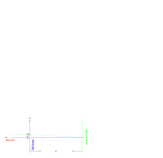
Figure 1: The illustration of one dimensional scattering screen.

2 The stationary phase approximation

We consider the wavefield from a point source at infinity to be incident up on a single thin, one-dimensional scattering screen, as described in figure 1. For an incident wavefield of unit amplitude the wavefield observed at the central position on the line a distance $z$ (${r_{\rm F}^{2}}=z/k$) from the scattering screen is (e.g. Born & Wolf 1980)

$$u(z)=\frac{1}{\sqrt{2\pi r_{\rm F}^{2}}}\int_{-\infty}^{\infty}d{x}\exp\left[i\left(\frac{x^{2}}{2r_{\rm F}^{2}}+\phi({x})\right)\right].$$ (1)

To solve this we employ the method of stationary phase (e.g. Mandel & Wolf, P.128), which states that an integral of the form,

$$F(k)=\int_{-\infty}^{\infty}f(x)e^{ikg(x)}\,dx,$$ (2)

has an approximation containing contributions from critical points inside the boundary of integration $(-\infty,\infty)$:

$$F(k)\sim\left(\frac{2\pi}{k}\right)^{1/2}\sum_{j=1}^{n}\frac{\epsilon_{j}}{|g^{\prime\prime}(x_{j})|^{1/2}}f(x_{j})e^{ikg(x_{j})},$$ (3)

where $\epsilon_{j}=e^{\pm i\pi/4}$    is according    as    $g^{\prime\prime}(x_{j})>0{\;}(<0)$ for + (-) and $x_{j}$ are the points of stationary phase which satisfy the condition $g^{\prime}(x_{j})=0.$ Applying the stationary phase approximation and $g(x)=k^{-1}(\phi(x)+x^{2}/2r_{\rm F}^{2})$ to Eq.(1), one has

$$u(z)\approx\sum_{j=1}^{N}u_{j}\;,\;\;\;u_{j}=\frac{\epsilon_{j}}{\sqrt{|1+r_{\rm F}^{2}\phi^{\prime\prime}(x_{j})|}}\exp[ir_{\rm F}^{2}\phi^{\prime 2}(x_{j})/2+i\phi(x_{j})].$$ (4)

It is noted that Eq.(3) or Eq.(4) is an approximate result, and it is assumed that g”(x) does not go to zero. The independent variables are the phasor $\phi$, its first derivative $\phi^{\prime}$, and the total number of them is 2N, where N is the SPP number. The mean intensity of the unit amplitude wave, $<I>=1$, is identified as the average value of the second moment of the amplitude $<uu^{*}>$. Adding a subscript $N$ to denote the number of SPPs, in the SPP approximation this is

$$<I>_{N}=\sum_{i,j=1}^{N}<u_{i}u^{*}_{j}>=\sum_{i=1}^{N}<u_{i}u^{*}_{i}>+\sum_{i\neq j=1}^{N}<u_{i}u^{*}_{j}>=1.$$ (5)

Thus the number of SPP is the maximum integer of N solved from Eq.(5). While considering a statistical model in which each SPP is assumed to come from a distribution, all SPPs are statistically equivalent. Then, for example, $<u_{i}u^{*}_{i}>$ may be written as $<u_{1}u^{*}_{1}>$, and the sum over $i=1,\ldots N$ gives $N<u_{1}u^{*}_{1}>$. Only two independent averages appear in the intensity, and we write these as

$$U_{11}=<u_{1}u^{*}_{1}>,\;U_{12}=(<u_{1}u^{*}_{2}>+<u_{2}u^{*}_{1}>)/2,$$ (6)

so that Eq.(5) reduces to

$$<I>_{N}=NU_{11}+N(N-1)U_{12}=1.$$ (7)

Similar to the procedure of treating the intensity, the intensity square is obtained as follows,

$$<I^{2}>_{N}=NU_{1111}+4N(N-1)U_{1112}+N(N-1)(U_{1122}+U_{1221}+U_{1212})$$

$$+N(N-1)(N-2)(4U_{1123}+2U_{1213})+(N-1)(N-2)(N-3)U_{1234}\;,$$ (8)

where the terms, such as $U_{1111}$ and $U_{1122}$, are the averaged values of the products of amplitudes and generally denoted by,

$$U_{jklm}=<jklm>=<u_{j}u_{k}^{*}u_{l}u_{m}^{*}>,$$ (9)

which satisfies,

$$<jklm>^{*}=<kjml>=<mlkj>,$$ (10)

so we have $U_{1122}=U_{1221}=U_{11}U_{22}=U_{11}^{2}$. Henceforth, the modulation index $m$ of diffraction is defined by

$$m=\sqrt{<I^{2}>_{N}-1}\;.$$ (11)

2.1 The calculations of the intensity in SPP

The power spectrum of the phase inhomogeneities, $\Phi(k)$, is assumed to have the following form (see e.g. Blandford & Narayan 1985; Goodman & Narayan 1985)

$$\Phi(k)=\left\{\begin{array}[]{ll}L_{0},&k<1/L\\ L_{0}(Lk)^{-\beta},&1/L<k<1/l\\ 0,&k>1/l\end{array}\right.,$$ (15)

where $\beta=8/3$ is an index for a Kolmogorov spectrum of turbulence with the structure constant $L_{0}$ and $l$ ($L$) is the inner (outer) scale. In addition, we assume the phase parameters to follow the Gaussian distribution $P(\psi)$, where $\psi$ represents the phase variables $\phi$, $\phi^{\prime}$ and $\phi^{\prime\prime}$,

$$P(\psi)=\frac{1}{\sqrt{2\pi\sigma_{\psi}^{2}}}\exp\left[-\frac{{\psi}^{2}}{2\sigma_{\psi}^{2}}\right],$$ (16)

where $\sigma_{\psi}$ is a standard deviation of the parameter $\psi$, calculated from the spectrum function of Eq.(15) (see Melrose & Watson 2006). Furthermore, the terms in intensity and intensity square expressions of Eq.(7) and Eq.(8) can be calculated by an integral of the probability distribution over the 6 random variables (see Melrose & Watson 2005), for instance,

$$<jk>=\langle u_{j}u_{k}^{*}\rangle=\int[\int_{0}^{\infty}d\phi_{j}^{\prime\prime}\int_{0}^{\infty}d\phi_{k}^{\prime\prime}+\int_{-\infty}^{0}d\phi_{j}^{\prime\prime}\int_{-\infty}^{0}d\phi_{k}^{\prime\prime}+\int_{0}^{\infty}d\phi_{j}^{\prime\prime}\int_{-\infty}^{0}d\phi_{k}^{\prime\prime}\,e^{i\pi/2}$$ (17)

$$+ \int_{-\infty}^{0}d\phi_{j}^{\prime\prime}\int_{0}^{\infty}d\phi_{k}^{\prime\prime}\,e^{-i\pi/2}]\frac{P(\phi_{j},\phi_{k},\phi_{j}^{\prime},\phi_{k}^{\prime},\phi_{j}^{\prime\prime},\phi_{k}^{\prime\prime})}{\left|1+r_{\rm F}^{2}\phi_{j}^{\prime\prime}\right|^{1/2}\,\left|1+r_{\rm F}^{2}\phi_{k}^{\prime\prime}\right|^{1/2}}\exp\left[iZ_{jk}\right]d\phi_{j}d\phi_{k}d\phi_{j}^{\prime}d\phi_{k}^{\prime}\;,$$

with

$$Z_{jk}=r_{\rm F}^{2}({\phi_{j}^{\prime}}^{2}-{\phi_{k}^{\prime}}^{2})/2+(\phi_{j}-\phi_{k})\;,$$ (18)

$$P(\phi_{j},\phi_{k},\phi_{j}^{\prime},\phi_{k}^{\prime},\phi_{j}^{\prime\prime},\phi_{k}^{\prime\prime})=P(\phi_{j})P(\phi_{k})P(\phi_{j}^{\prime})P(\phi_{k}^{\prime})P(\phi_{j}^{\prime\prime})P(\phi_{k}^{\prime\prime}).$$ (19)

3 results and discussions

The numerical results of the modulation index versus the scattering strength $r_{\rm F}/r_{\rm diff}$ are shown in figure 2. We find that the modulation index increases with the scattering strength continually from the weak scattering regime, via the transitional scattering regime, to the strong scattering regime where the modulation index is fully saturated. The influence by the inner scale on the modulation index is studied, and we find that the increasing of inner scale makes the modulation index decrease a little at the transitional scattering regime but little effect in the strong scattering regime. The trends of the modulation index in the weak and strong scattering regimes are similar to those obtained by the approximated treatments (see. e.g. Narayan 1992; Rickett 1977, 1990), however the SPP method provides the descriptions of modulation index at the transitional scattering. If N=1, a weak scattering case, we have

$$m\approx U_{1111}/U_{11}^{2}-1\;,$$ (20)

from which we can obtain that the modulation index increases with the scattering strength $r_{\rm F}/r_{\rm diff}$, similar to the case discussed by Salpeter (1967) (Melrose & Watson 2005). In the transitional scattering the number N is about 2 or 3 but depends on the choice of inner scale. If $N\rightarrow\infty$, a strong scattering case, we find that the interchange terms of amplitude products, for instance $<jklm>$ with j,k,l and m being not all same, are very small and $U_{1111}\sim U_{1122}\sim U_{1221})\sim 1/N^{2}$. Therefore, the following approximation is preserved,

$$m=<I^{2}>_{N}-1\simeq NU_{1111}+N(N-1)(U_{1122}+U_{1221})-1\simeq 1\;,$$ (21)

a fully modulated scintillation, which has been obtained and discussed by Gwinn et al. (1998).

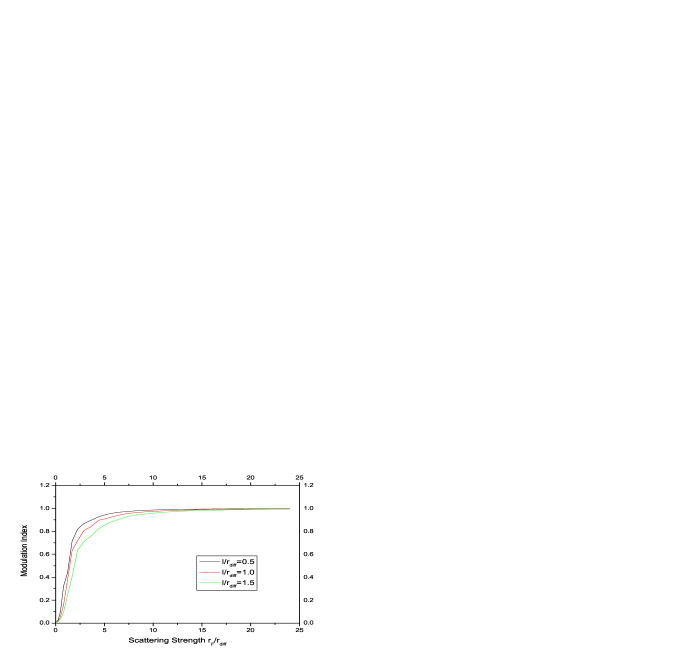
Figure 2: Modulation index v.s. scattering strength $r_{\rm F}/r_{\rm diff}$. The influence by the inner scale of ISM is plotted as indicated in the figure.

Moreover, there exists a discrepancy between our results and those earlier results by Goodman and Narayan (2005) who found the modulation index m$>$1 at transitional scattering regime, which calls into question the reliability of the SPP method. Or it may possibly be due to the 1-D nature of our computation, which could be resolved by applying the method to a 2-D screen in a future work.

Acknowledgments Thanks are due to many helpful discussions with D.B. Melrose, B. Rickett , D. Stinebring, M. Walker, J.P. Macquart, N. Wang and X.J. Wu.

References

Armstrong J.W., Rickett B.J., Spangler S.R. 1995, ApJ, 443, 209

Blandford, R.D. & Narayan, R., 1985, MNRAS, 213, 591

Cordes J.M., Weisberg J.M., Boriakoff V. 1985, ApJ, 288, 221

Goodman, J.J., & Narayan, R. 1985, MNRAS, 214, 519

Goodman, J.J., & Narayan, R. 2005, ApJ, 636, 510

Gwinn, C.R. et al. 1998, ApJ, 505, 928

Kaspi, V. M., & Stinebring, D.R. 1992, ApJ, 392, 530

Lyne, A.G., & Smith, F.G. 2005, Pulsar Astronomy, Cambridge University Press

Manchester, R.N., Taylor, J.H. 1977, Pulsars, Freeman, San Fransisco

Mandel, L. & Wolf, E. 1995, Optical Coherence and Quantum Optics, Cambridge University Press

Melrose, D.B., & Watson, P. 2006, ApJ, 647, 1131

Narayan, R. 1992, Phil. Trans. R. Soc. Lond. A, 341, 151

Rickett, B.J. 1977, ARAA 15, 479

Rickett, B.J. et al. 1984, A&A 134, 390

Rickett, B.J. 1990, ARAA 28, 561

Rickett, B.J. 2006, ChJAA, 6, Suppl 2.

Salpeter, E.E., 1967, ApJ, 147, 433

Scheuer, P.A.G. 1968, Nat 218, 920

Stinebring, D.J., et al. 2000, ApJ, 539, 300